Application of the Weighted K-Nearest Neighbor Algorithm for Short-Term Load Forecasting

Abstract

In this paper, the historical power load data from the National Electricity Market (Australia) is used to analyze the characteristics and regulations of electricity (the average value of every eight hours). Then, considering the inverse of Euclidean distance as the weight, this paper proposes a novel short-term load forecasting model based on the weighted k-nearest neighbor algorithm to receive higher satisfied accuracy. In addition, the forecasting errors are compared with the back-propagation neural network model and the autoregressive moving average model. The comparison results demonstrate that the proposed forecasting model could reflect variation trend and has good fitting ability in short-term load forecasting.

1. Introduction

Short-term load forecasting is used to forecast the power loads in the coming months, weeks, or even shorter, with greater accuracy than long-term load forecasting. In the competitive power market, the forecasting accuracy directly affects the economic cost of operators, so it occupies an important position in modern power demand management [1]. According to the data of short-term load forecasting, it not only can optimize the combination of generator sets, economic dispatching, and the power flow calculation for power generation, but also can guarantee the economical safe operations of the power system [2].

Classical deterministic theories are mainly applied to conduct the traditional short-term load forecasting. Such as time series method [3], back-propagation neural network (BPNN) model [4], gray model [5,6], and support vector regression [7,8,9], etc. Although these methods are widely adopted, there are still some outstanding problems, for example, (1) it is difficult to simulate the relationships between the variables affecting the electricity loads and the loads themselves by accurate mathematical model; (2) the forecasting accuracy requires improvements; (3) the forecasting effect is not satisfied; and (4) the real situation of the electricity load cannot be reflected in real time. Therefore, it is of great practical significance to study and establish a more accurate and intuitive short-term load forecasting model.

Recently, Martínez-Álvarez et al. [10] indicate the importance of pattern sequence similarity, and introduce the pattern sequence-based forecasting (PSF) algorithm, which contains clustering (selection of the optimum number of clusters) and prediction (like optimum window size selection for specific patterns and prediction of future values). Later, Bokde et al. [11] published the R code for modeling. Due to the similar theoretical designing of PSF, the k-nearest neighbor (K-NN) algorithm [12] is a mature theoretical tool and is easily implemented. It is often used to solve nonlinear problems, such as credit ratings and bank customer rankings, in which the collected data do not always follow the theoretical linear assumption, thus it should be one of the first choices when there is little or no prior knowledge about the distribution data. In addition, it can successfully reduce the influences of the variables on the experimental processes [13]. It has higher forecasting accuracy and has no assumptions for the collected data, and particularly, it is not sensitive to the outliers. It has been widely applied in real-world problems, such as analyzing the structure of the stock market [14], fault detection and diagnosis for photovoltaic systems [15], and social images recognition in social networks [16]. In addition, several improved K-NN algorithms have also been explored, for example, Zhang et al. [17] propose an improved K-NN algorithm by reconstructing a sparse coefficient matrix between test samples and training data to keep the local structures of data for achieving the efficiency. Their proposed improved K-NN algorithm is applied to classification, regression, and missing data imputation with superior results. Bhattacharya et al. [13] employs the weights obtained from the analytic hierarchy process (AHP) for different features to propose a weighted distance function for the K-NN algorithm. Their results demonstrate that the performance of the proposed K-NN classifier can receive improved results in terms of pairwise comparison of features.

The original W-K-NN forecasting algorithm was developed and introduced by Troncoso et al. in 2007 [18]. Thereafter, several researchers have considered empowering weight for each nearest neighbor [19], for instance, Chen and Hao [20] proposed a support vector machine (SVM)-based weighted K-NN algorithm to effectively predict stock market indices by using support vector machines to obtain the associated weight for each feature. Their forecasting results are better than other models. Biswas et al. [21] propose the parameter independent fuzzy class-specific feature weighted K-NN (PIFW-K-NN) classifier, in which, the class dependent optimum weight is based on the distances from the query point using a fuzzy membership function. Their classification results demonstrate the improved accuracy of the proposed PIFW-K-NN than other state-of-the-art classifiers. Su [22] proposes the weighted K-NN (W-K-NN) by hybridizing the genetic algorithm with K-NN (k-nearest neighbor) to detect large-scale attacks. The weight for each nearest neighbor is weighted by Euclidean distance, then, the genetic algorithm (GA) is used to find an optimal weight vector for all nearest neighbors. Their results demonstrate that the detection accuracy is improved significantly. Lei and Zuo [23] also propose the weighted K-NN (W-K-NN) classification algorithm by using Euclidean distance evaluation technique (EDET) to select sensitive features and remove fault-unrelated features. The applied results of the proposed method demonstrate its effectiveness. Ren et al. [24] propose a weighted sparse neighbor algorithm based on Gaussian kernel function to resolve face recognition problems. In which, the weights are calculated distance-based on Gaussian kernel to measure the similarity between test sample and each training sample. Their results demonstrate that the proposed algorithm could reach a higher recognition rate than other existing alternative models. Recently, Mateos-García et al. [25] propose the simultaneous weighting of attributes and neighbors (SWAN) to improve the classification accuracy, by using an evolutionary computation technique to adjust the contribution of the neighbors and the significance of the features of the data. Their results demonstrate that the proposed SWAN is superior to other alternative weighted K-NN methods. Llames et al. [26] propose a new approach for big data forecasting based on the weight K-NN to conduct distributed computing under the Apache Spark framework, in which four different weight calculations are employed. A Spanish energy consumption big data time series (measured every 10 min for nine years) has been used to test the algorithm. The results also support the superiority of the proposed weight K-NN model.

Based on above relevant literature reviews, the inverse of Euclidean distance is employed as the weight, then, it is hybridized with the K-NN algorithm (namely W-K-NN algorithm) to improve the forecasting accuracy. Thus, this paper proposes a short-term load forecasting model based on the new parametrization of the W-K-NN algorithm so that it is adapted to China patterns: (1) According to a known sample set, forecast the electricity loads at a certain time; (2) calculate the Euclidean distance using its proximity data, the reciprocal of the calculated distance is used to determine the weight for each data point; (3) the closer the distance, the greater the weight, thus the data points can be better classified and the short-term load can be better forecasted. Comparing the model structure with the similar works proposed by Llames et al. [26], Rana et al. [27], and Troncoso et al. [28], which use 10-min electricity demand, hourly electricity load, and price, respectively, for one day ahead to calculate the weight by the distance of the neighbors. On the contrary, the proposed model in this paper can extract the inertia of the electricity consumption behaviors from larger historical load data (i.e., the normal production life cycle in China: three load data patterns for each eight hours in a day) to calculate the weights by the reciprocal of the distance, which also avoid being bounded in the characteristics of the short cycle. It can be emphasized that the proposed model is based on the state space and the production life cycle to determine the weights, which can capture the weight more accurately.

The rest of this paper is organized as follows. In Section 2, the details of the K-NN algorithm are introduced briefly. In Section 3, a short-term load forecasting model based on the W-K-NN algorithm is proposed and the main steps of the proposed model are also illustrated. In Section 4, the proposed model is simulated and compared with two common alternative models (i.e., the autoregressive-moving average (ARMA) and the BPNN models). In Section 5, a brief conclusion of this paper and the future research are provided.

2. The K-NN Algorithm

The K-NN algorithm is proposed to find out k training samples that are closest to the target object in the training set. Furthermore, determine the dominant category from the k training samples; then, assign this dominant category to the target object, where k is the number of training samples.

Therefore, the principal mechanism of the K-NN algorithm is that all samples have the same characteristics while they are classified in the same category in a feature space, which the category contains the k most neighboring samples. In determining the classification decision, the method determines the category to which the sample belongs only according to the category of the nearest one or several samples. In addition, the K-NN algorithm is only relevant to a very small number of adjacent samples in category decision making. Since the K-NN algorithm mainly relies on the surrounding limited adjacent samples, rather than relying on the method of discriminant domain method to determine the category, thus the K-NN algorithm is more suitable than other methods for the pending sample sets where the class domain crosses or overlaps more. The idea of the K-NN algorithm is demonstrated in Figure 1. In which, $X_u$ belongs to the category (${\omega }_1$) because four neighboring samples belong to ${\omega }_1$, only one neighboring sample belongs to ${\omega }_3$.

The specified implementation process of the K-NN algorithm contains the following six steps,

(1)

Select the k value;

(2)

Calculate the distance between the point in the known category data set and the current point;

(3)

Sort in increasing order of distance;

(4)

Select k points with the smallest distance from the current point;

(5)

Determine the frequency of occurrence of the category in which k points are located;

(6)

Return to the category with the highest frequency of occurrence of the first k points as the predicted classification of the current point.

The K-NN algorithm needs to calculate the distance between the forecasted data point and the known data point, so as to the select the nearest k labeled data, $\left\{y_1,y_2,\dots ,y_k\right\}$, where $y_1$ represents the known data point closest to the forecasted point; $y_2$ represents the known data point that is the second closest to the forecasted point, and so on. Therefore, the short-term load forecasting can be conducted by the K-NN algorithm regression as Equation (1),

$${\mathrm{s}}_i=\frac{1}{k}\times {\displaystyle \sum }_{j=1}^k{s}_{y_j}$$

(1)

where ${\mathrm{s}}_i$ represents the ith forecasted value, which is the average value of $s_{y_j}$ ($j=1,2,\dots ,k$); $s_{y_j}$ represents the forecasted value of the jth closest known data point ($y_j$).

3. Short-Term Load Forecasting Model Based on W-K-NN

In order to establish the short-term load forecasting model based on the proposed W-K-NN algorithm, the specified implementation process contains the following three steps, and the associated flow chart is demonstrated in Figure 2.

(1)

Selection of the value of k. For a research sample (S) in its associated feature space, most of the K nearest adjacent samples belonged to a certain category, and the sample, S, also belonged to this category. Then, the appropriate nearest neighbor parameter, k, is selected based on the characteristics of the research samples in this category. In which the characteristics mean that similar historical electricity consumption behaviors will definitely form agglomeration in a certain space.

(2)

Construct the theoretical sample set and output set. Based on the principle of random distribution (to ensure all historical electricity consumption behaviors are likely to be traversed not limited to the local optima), calculate the Euclidean distance between the forecasted data point and the known data point. Then, the reciprocal of the distance is used as the weight for each forecasted data point. Eventually, the forecasted value of each data point could be received (by Equation (6), refer Section 3.2).

(3)

Forecasting accuracy evaluation. To verify the forecasting accuracy, the root mean square error (RMSE) and the normalized mean square error (NMSE) are employed as the principal evaluation indexes. They are calculated as Equations (2) and (3), respectively. The smaller the value for the forecasting errors, the more accurate the forecasting results. Thus, the forecasting results, computed by MATLAB software R2017a version, would be used to calculate the forecasting errors with the actual data values, the reliability and the forecasting accuracy of the proposed model would be further verified.

$$\mathrm{RMSE}=\sqrt{\frac{{{\displaystyle \sum }}_{i=1}^N{\left(a_i-s_i\right)}^2}{N-1}}$$

(2)

$$\mathrm{NMSE}=\frac{{{\displaystyle \sum }}_{i=1}^N{\left(a_i-s_i\right)}^2}{\sqrt{N}{{\displaystyle \sum }}_{i=1}^N{\left(a_i-\overline{a}\right)}^2}$$

(3)

where ${\mathrm{s}}_i$ represents the ith forecasted electricity load value; $a_i$ represents the ith actual electricity load value; $\overline{a}$ represents the mean value of N actual electricity load values; N represents the total number of forecasted electricity load.

To demonstrate the universal applicability of the proposed model, the data are divided into large sample and small sample, respectively. The large sample is divided by quarter (i.e., in each quarter, the data of the first two months are used as the theoretical modeling samples to forecast the electricity load values of the third month). The small sample is divided by month (i.e., in each month, the data of the first three weeks are used as the theoretical modeling samples to forecast the electricity load values of the fourth week).

The following two sub-sections would introduce the details of the first two steps.

3.1. Selection of the Value of k

Based on the K-NN algorithm, k is a user-defined neighbor parameter, which is used to classify samples to be classified according to the category label with the highest frequency of occurrence among the k training samples that are closest to the selected data point. If the value of k is too large or too small, it will increase the interference to the data and reduce the classification accuracy. In the case where the value of k is small, the complexity of the model is higher (i.e., it is easy to suffer from the over-fitting problem), and there is an increase of the estimation errors. Eventually, the forecasting results are very sensitive to the neighbor data points. On the contrary, in the case where the value of k is large, it would reduce the estimation errors; however, the approximation errors would be simultaneously increased, and the training data points farther from the input data point will also affect the forecasting results. Therefore, in general applications of the K-NN algorithm, the value of k is often set as a relatively small value, but must be an integer.

In this paper, the trial and error method was adopted to observe the experimental results and to determine the suitable value of k (i.e., the determined value of k were fixed during the forecasting processes). For example, the determined suitable values of k for small samples and large samples are illustrated in

Table 1. Comparison of the errors of different nearest neighbor numbers (the value of k) in small samples (unit: MW).

Forecasting Period	k = 1		k = 2		k = 3
	RMSE	NMSE	RMSE	NMSE	RMSE	NMSE
Jan.	853.27	0.39	586.03	0.18	798.43	0.41
Feb.	367.07	0.08	342.87	0.07	413.52	0.12
Mar.	1081.62	0.95	636.97	0.33	903.17	0.76
Apr.	415.30	0.20	435.60	0.22	466.76	0.25
May.	347.23	0.12	415.28	0.17	423.52	0.17
Jun.	302.43	0.05	230.31	0.03	326.34	0.06
Jul.	571.71	0.32	585.92	0.34	631.41	0.39
Aug.	1146.88	1.24	825.47	0.64	780.13	0.57
Sep.	467.92	0.28	485.79	0.30	554.39	0.51
Oct.	1917.09	0.90	1885.15	0.87	1883.64	0.86
Nov.	343.61	0.10	320.80	0.08	229.73	0.04
Dec.	1324.44	0.89	1106.39	0.62	1111.05	0.63

and

Table 2. Comparison of the errors of different nearest neighbor numbers (the value of k) in large samples (unit: MW).

Forecasting Period	k = 1		k = 2		k = 3
	RMSE	NMSE	RMSE	NMSE	RMSE	NMSE
Mar.	868.63	0.48	857.60	0.46	864.07	0.47
Jun.	1433.48	0.56	1369.56	0.45	1458.62	0.51
Sep.	497.69	0.15	553.51	0.18	656.58	0.25
Dec.	1148.63	0.99	814.08	0.50	744.02	0.42

, respectively. In which, the small samples were based on the electricity loads for three weeks; the large samples were based on two months.

Based on the comparison of the experimental results in Table 1 and Table 2, it was found that when k was determined as 2, the experimental error was relatively small and the fitting effect was good.

3.2. Weights Calculation and New Forecasting Values

As mentioned in Section 3.1, if the nearest neighbor number, k, is determined as 2, then the Euclidean distance between the forecasted data point ($s_j$) and the known data point ($y_j$) was calculated by Equation (4).

$$d_{i,y_j}=\sqrt{{\displaystyle \sum }_{j=1}^k{\left(s_j-y_j\right)}^2}$$

(4)

The weight for each forecasted data point was calculated by the reciprocal of the distance, as shown in Equation (5).

$$w_{i,y_j}=\frac{1}{d_{i,y_j}}$$

(5)

Then, the final forecasted value ($s_i^{\prime }$) of each data point was calculated by Equation (6).

$$s_i^{\prime }=\frac{{{\displaystyle \sum }}_{j=1}^k{w}_{i,y_j}\times s_{y_j}}{{{\displaystyle \sum }}_{j=1}^k{w}_{i,y_j}}$$

(6)

Finally, the proposed W-K-NN model was used to forecast the electricity load values of the third month (for the large sample) and the electricity load values of the fourth week (for the small sample), respectively.

3.3. Forecasting Accuracy Evaluation Indexes

As mentioned above, RMSE (Equation (2)) and NMSE (Equation (3)) were used to evaluate the forecasting accurate level in this paper. In addition, for comparing with other models in existing paper, two other evaluation indexes were also employed: (1) the mean absolute error (MAE); and (2) the mean absolute percentage error (MAPE). They are calculated as Equations (7) and (8), respectively.

$$\mathrm{MAE}=\frac{1}{N}{\displaystyle \sum }_{i=1}^N\left|a_i-s_i\right|$$

(7)

$$\mathrm{MAPE}=\frac{1}{N}{\displaystyle \sum }_{i=1}^N\left|\frac{a_i-s_i}{a_i}\right|\times 100\%$$

(8)

where ${\mathrm{s}}_i$ represents the ith forecasted electricity load value; $a_i$ represents the ith actual electricity load value; $\overline{a}$ represents the mean value of N actual electricity load values; N represents the total number of forecasted electricity load.

Via the accuracy evaluation indexes, such as the RMSE and the NMSE, the degree of variation and dispersion of the forecasting results could be further explained, and compared, so as to verify the reliability and accuracy of the model.

4. Results and Discussions

4.1. Forecasting Results and Analysis

The proposed W-K-NN model performed the forecasting processes and the associated results. The employed electricity load data were acquired from National Electricity Market (NEM, Australia), in total 1095 electricity load data, and data time period was from 8:00 on 1 January 2007 to 0:00 on 1 January 2008. In this paper, the collected data were based on an eight-hour scale (i.e., mean value of every eight hours), which often adopts the eight-hour work system (i.e., three shifts), as shown in

Table 3. The eight-hour scale for three stages in a day.

Stages	Time Periods	Real Statuses	Measurements
Stage 1	0:00 to 8:00	The period is at night	Mean load value of these eight hours
Stage 2	8:00 to 16:00	The period is the first half of a day
Stage 3	16:00 to 0:00	The period is the next half day

. The electricity load forecasting values of the third month (for the large sample) or of the fourth week (for the small sample) were obtained by the proposed W-K-NN model, the associated forecasting results are demonstrated in Figure 3 (large sample) and Figure 4 (small sample), respectively.

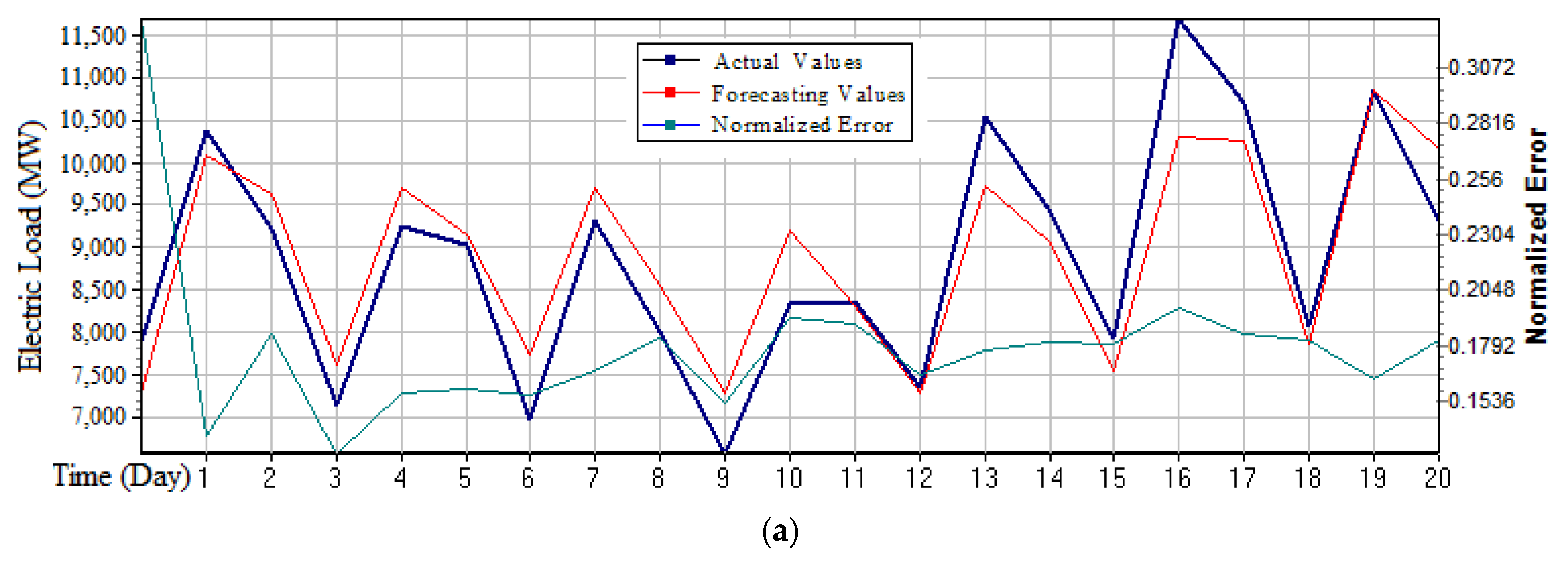
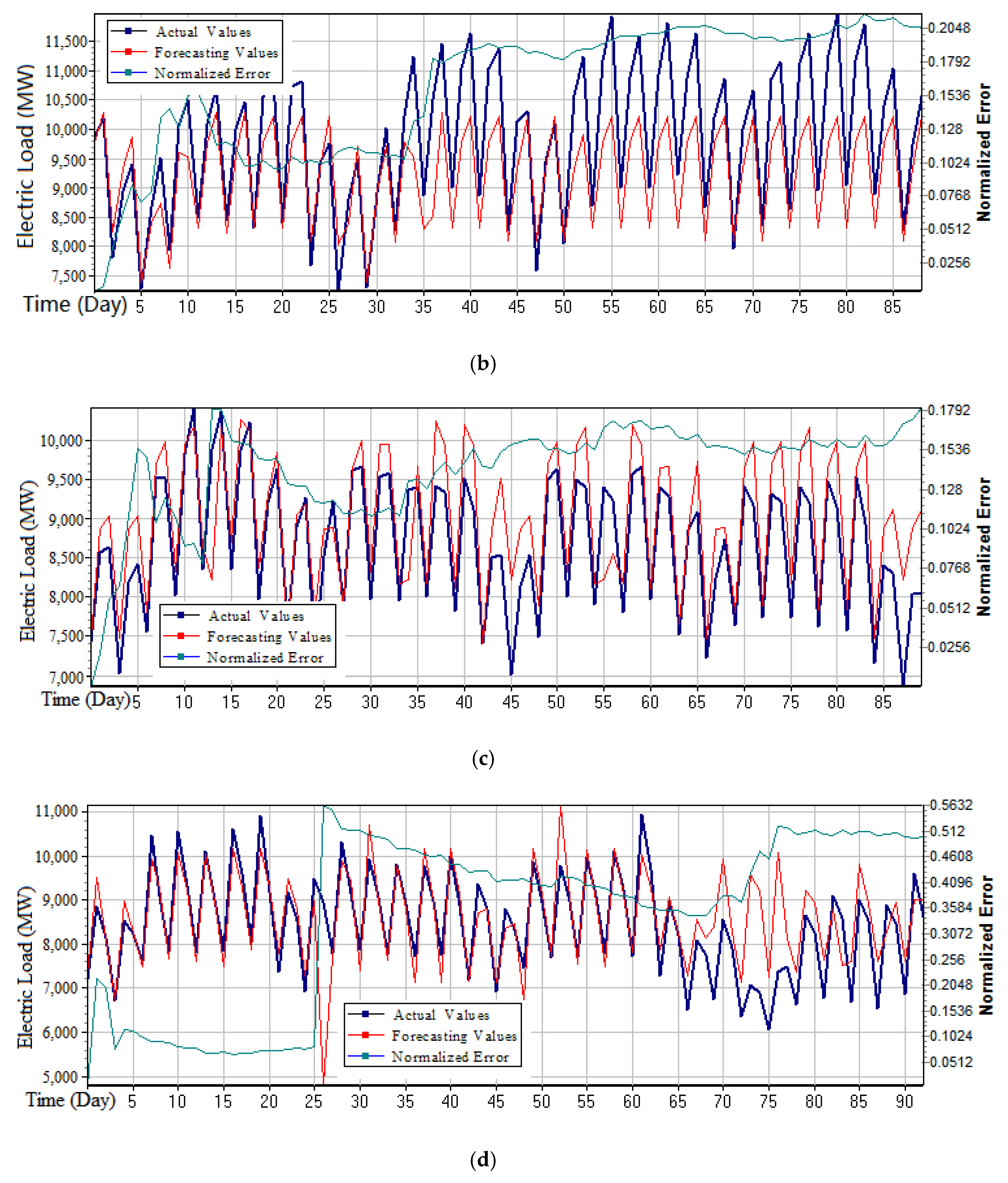
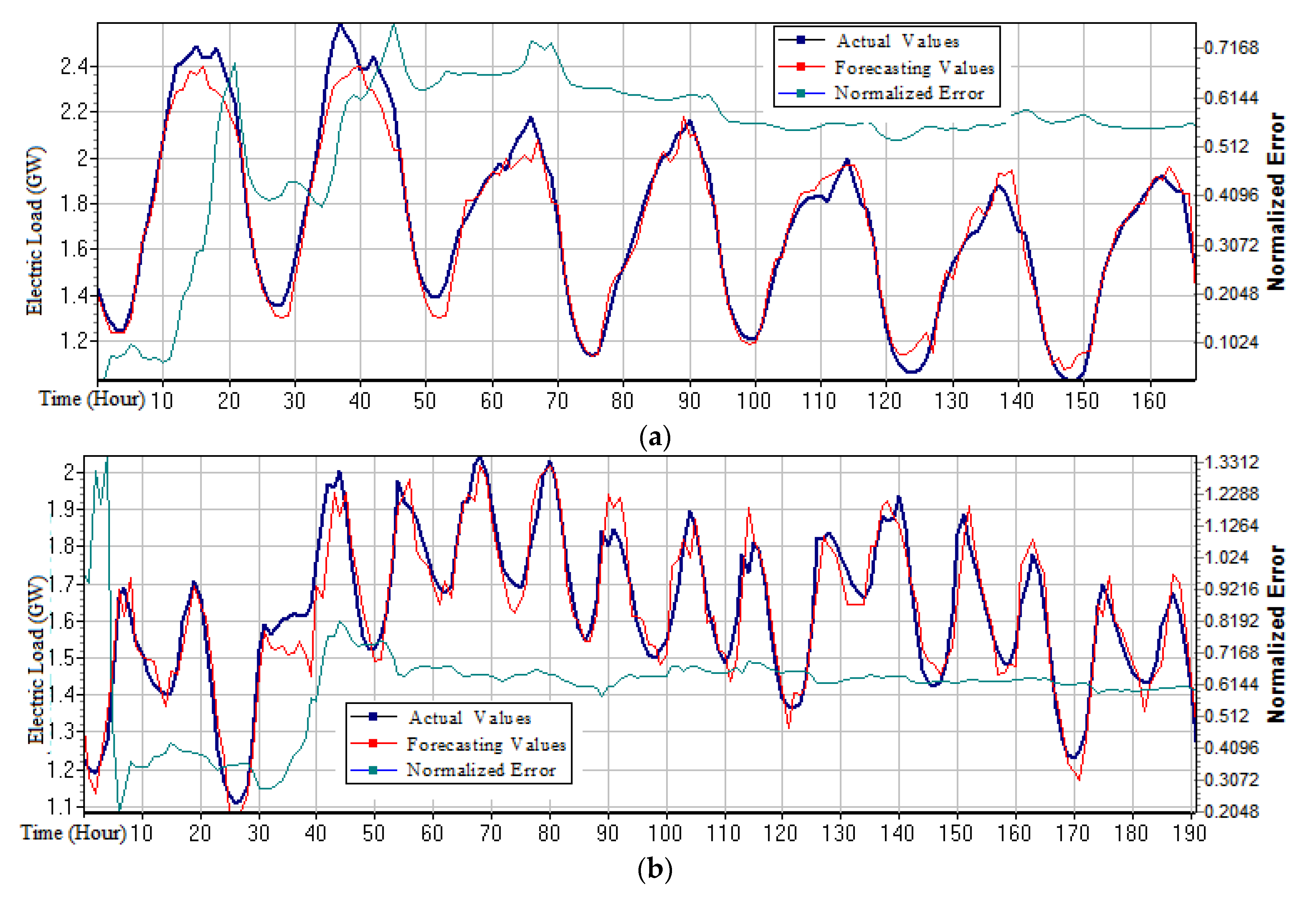
It can be learned from Figure 3 that the forecasting curve changed periodically, due to the three-stage-division of the data in a day. The first stage was from 0:00 to 8:00 (i.e., the period is at night, also is the origin in the figures); the second stage was from 8:00 to 16:00 (i.e., that is the first half of a day, the first point in the figures); and, the third stage was from 16:00 to 0:00 (i.e., that is the next half of a day, the second point in the figures. The three stages form a cycle (i.e., one activity cycle); in addition, a work cycle contains a total of seven cycles. The specific characteristics of electricity used in a cycle could be illustrated as follows: (1) The night was from 0:00 to 8:00, the residents’ daily electricity and educational electricity were at their lowest valley; the industrial electricity consumption was also small, so the lowest value of electricity consumption would occur during this period. (2) Start working at 8:00 in the morning, so the electricity consumption would gradually increase, until reaching the peak. (3) After 16:00, according to the production capacity demand plans, industrial production work load was generally reduced, so the electricity consumption would gradually decline.

Based on above observations, the trend of the curve variation in Figure 3 is in line with the actual electricity consumption. The third stage forecasting curve of each cycle in Figure 3a deviates from the actual curve, it may be caused from: (1) increased demand at this stage; or (2) a sudden increase in the workload of industrial production. Therefore, it can be learned from Figure 3 that the trend of the actual data and the forecasting data were generally consistent. Although there were certain errors, it was in line with the actual situation, and it indicates that the proposed W-K-NN model is suitable for short-term neighbor behavior detection, impact characterization, and could be weighted by the collected information, and, eventually, provide more effective and accurate forecasting results.

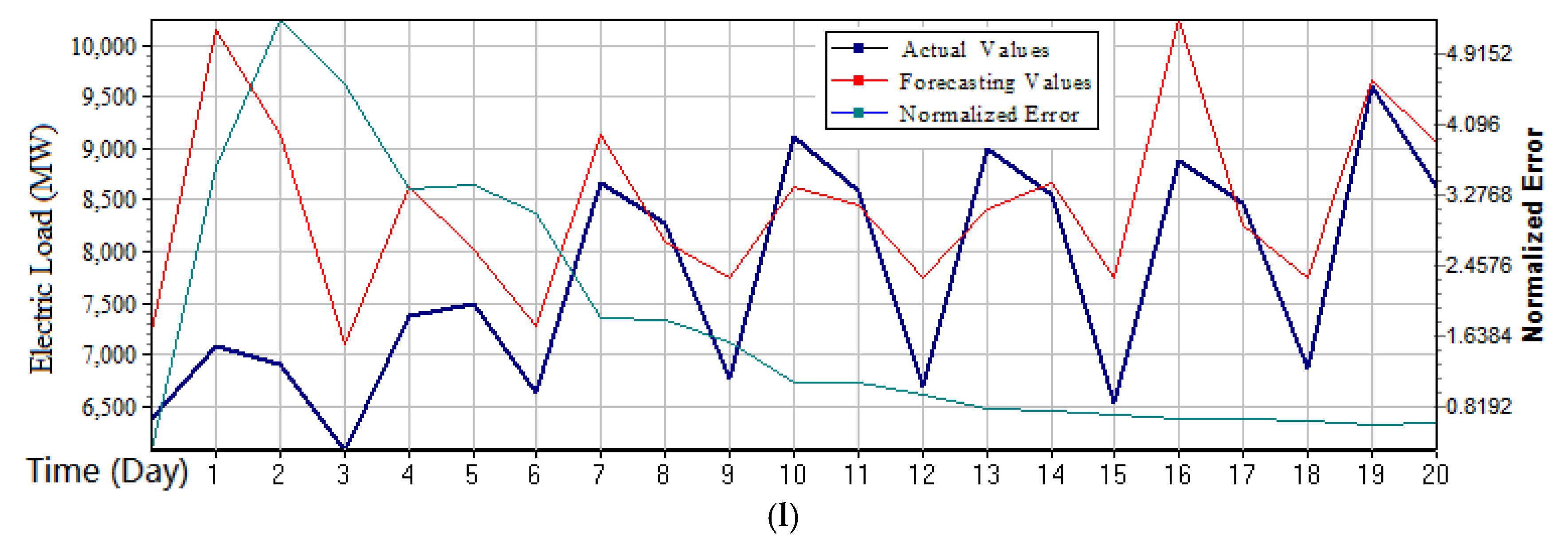
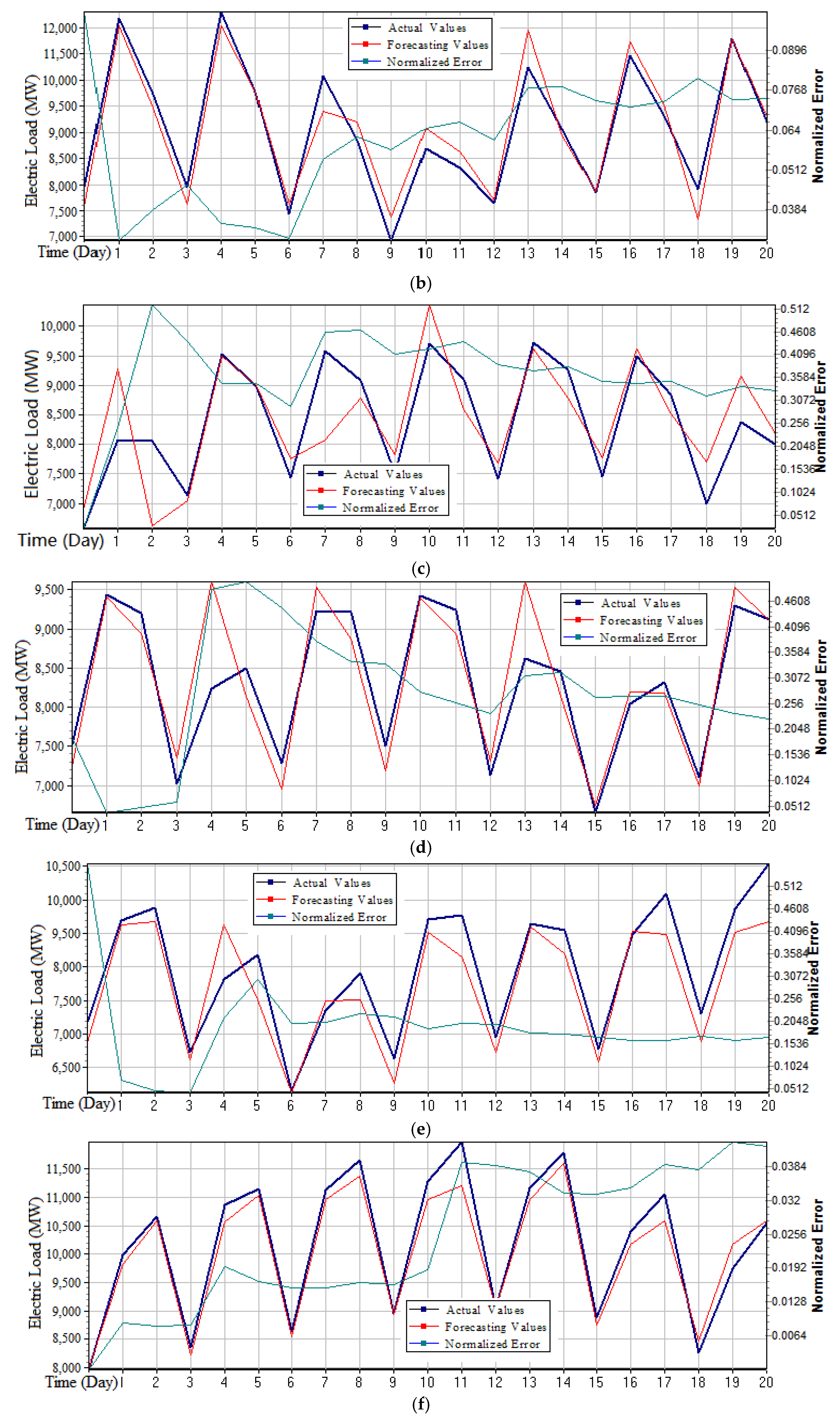
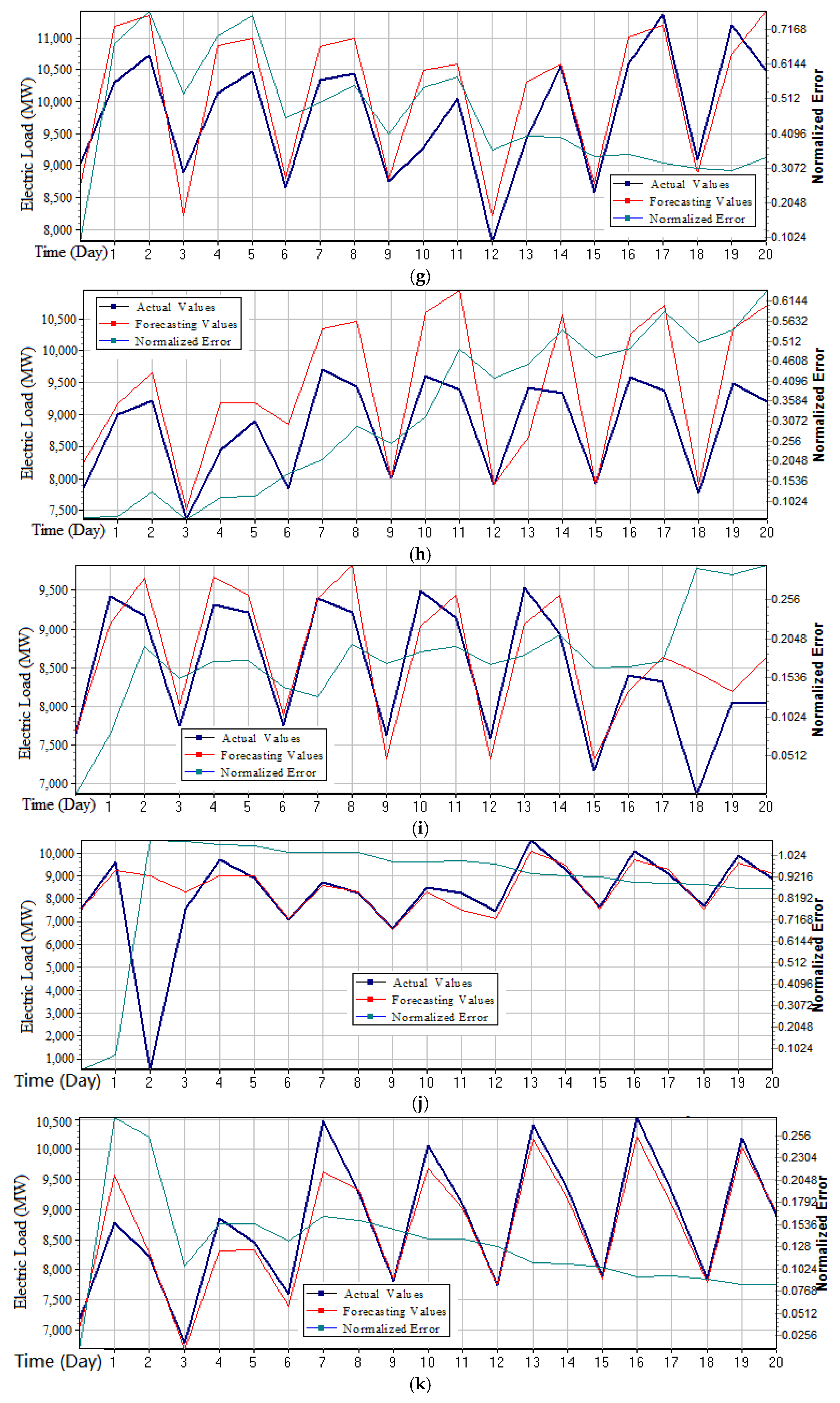
It can be learned from Figure 4, that the forecasting data curve demonstrates a rising and downward trend of cyclical variation, and consists of the actual data change trend. Similar to the small sample, the day data was also divided into three stages: from 0:00 to 8:00 (the first stage), from 8:00 to 16:00 (the second stage); and from 16:00 to 0:00 (the third stage). According to the arrangement of one day’s workload, it can reflect the cyclical variations, which indicates that this model can effectively reveal the rules of electricity consumption activities in each divided time period, particularly in the lowest points (i.e., the valley period). It demonstrates that this model can detect the information of the demand turning point (i.e., the demand is greater than the production capacity of the enterprise in this moment). Therefore, at this moment (valley period), for the power sector, it needs to organize production to simultaneously take into account market’s needs and own resources, managers should use their relatively fixed production capacity to meet changing market needs, such as several units are used to complete the power generation task.

Based on above observations, it can be seen from the Figure 4a,d that their fitting effects were good, while in Figure 4b,c, the fitting process shows a certain deviation, especially when the demand was turning to decrease (i.e., the top point, or the peak point), the fitting performance was not good. It also demonstrates that this model found it difficult to detect the oversupply information from the market. It was also affected by uncertain factors such as vacation and work plan; however, the error was not large and was within the controllable range.

4.2. Forecasting Results Comparison

In order to demonstrate the superiority of the proposed model, the ARMA model and BPNN model were selected for comparison analysis. The comparison results for both small sample and large sample are shown in Tables 5 and 6, respectively.

The following brief the modeling processes for these two employed models.

ARMA model is one of the most common time series models, it is widely used in economic field forecasting. The ARMA model principle is to regard the data sequence formed by the forecasting index over time as a random sequence. The dependence of this random sequence reflects the continuity of the original data in time. On the one hand, the influencing factors are relatively fixed and are easily expressed and explained. On the other hand, it has its own regulations of change, and the inertia is easily described. Therefore, the ARMA model was used to compare with the proposed W-K-NN model. By using MATLAB software R2017a version, after multiple tests, the AR order was determined to be 3. The electricity load forecasting values of the third month (for the large sample) could be obtained by using the data of the first two months, or, of the fourth week (for the small sample) could be obtained by using the data of the first three weeks. Then, the forecasting accuracy indexes, the RMSE and the NMSE (Equations (2) and (3)), were employed to calculated the forecasting accuracy for each case.

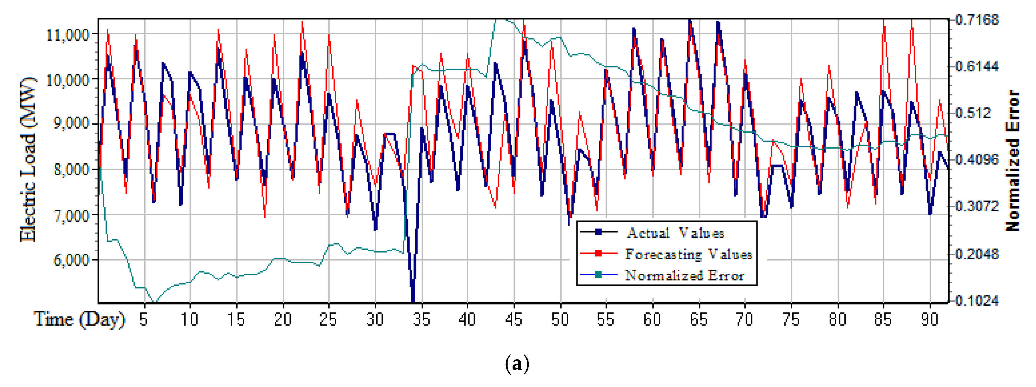
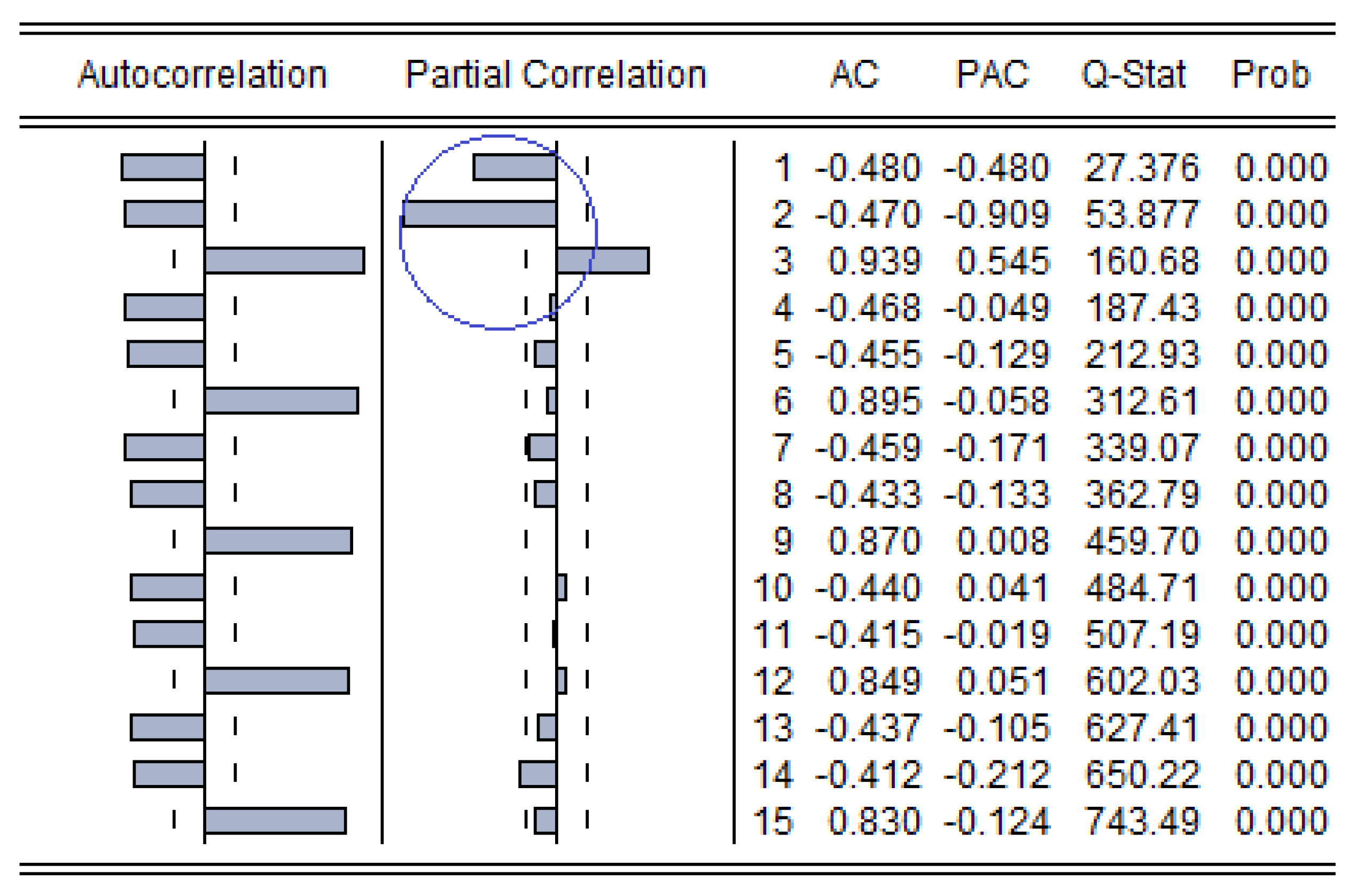
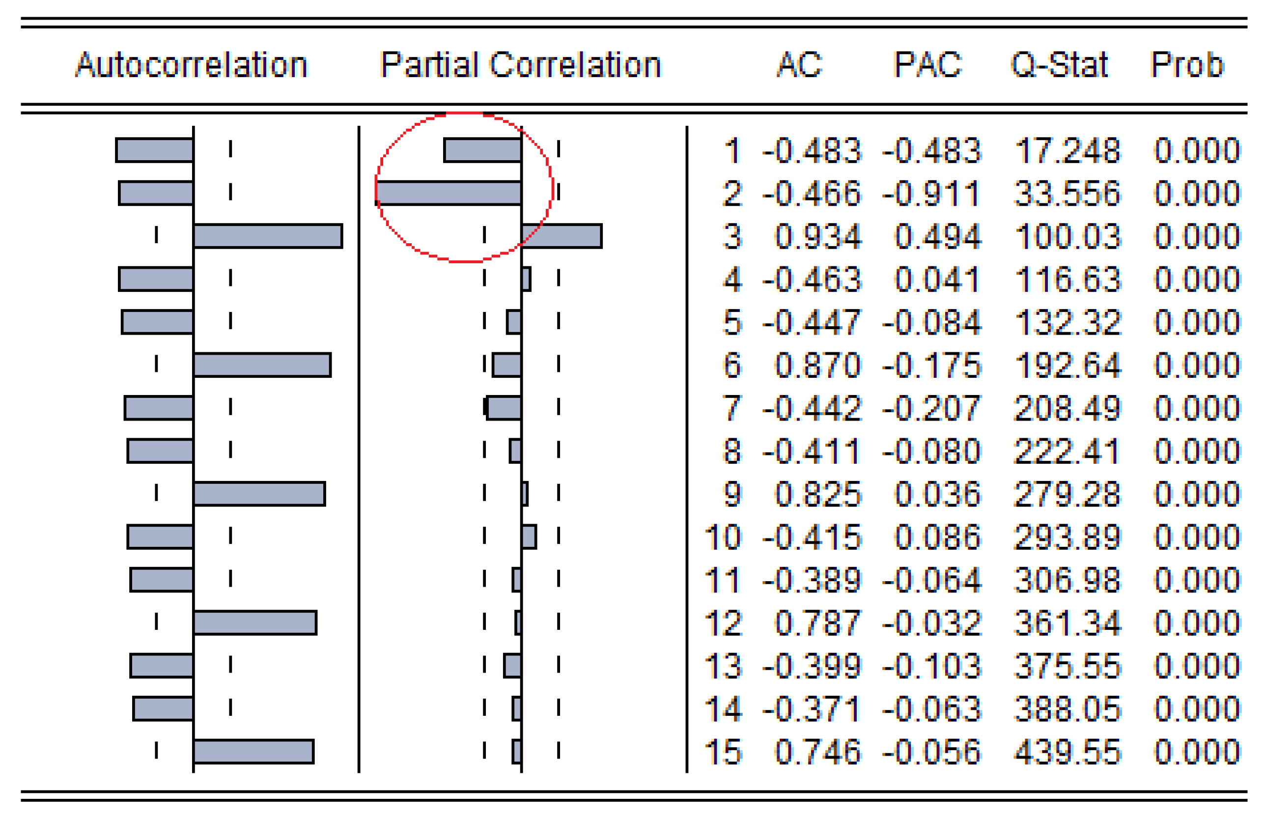
In general, for the stationary time series, the forecasting model could be determined from the auto-correlation function (ACF) and the partial auto-correlation function (PACF), the judgment criteria of the ARMA model are shown in

Table 4. Summary of ARMA model recognition graph judgment method.

Functions	AR (p)	MA (q)	ARMA (p,q)
ACF	tailing	trailing after q period	tailing
PACF	trailing after p period	tailing	tailing

. The ACF and the PACF graphs for the small sample and the large sample are illustrated in Figure 5 and Figure 6, respectively. It can be easily found that, in both samples, the ACF was trailing and the PACF was truncated, and there was a large attenuation after the third order (Figure 5 is outside the blue circle, while Figure 6 is outside the red circle). Thus, the AR (3) model was selected.

In Figure 5 and Figure 6, the ACF was defined as the correlation between time series $y_t$ and $y_{t-j}$, as shown in Equation (9),

$${\rho }_j=\frac{cov\left(y_t-y_{t-j}\right)}{\sqrt{var\left(y_t\right)}var\left(y_{t-j}\right)},\hspace{1em}\hspace{1em}j=0, \pm 1, \pm 2, \dots \dots$$

(9)

The PACF was defined as the correlation between $y_{t-1}$, $y_{t-2}$, …, and $y_{t-k+1}$. Q-statistics was defined as Equation (10),

$$\mathrm{Q}=n{\displaystyle \sum }_{k=1}^m{\widehat{\rho }}_k^2$$

(10)

where n is the number of the forecasting points; m is the delay points.

Q-statistics would be approximated to Chi-square (${\chi }^2$) distribution with m-degree of freedom; therefore, the decision rule is “Q-statistics is larger than ${\chi }_{1-\alpha }^2\left(m\right)$” or “p-value is smaller than significant level ($\alpha$)”.

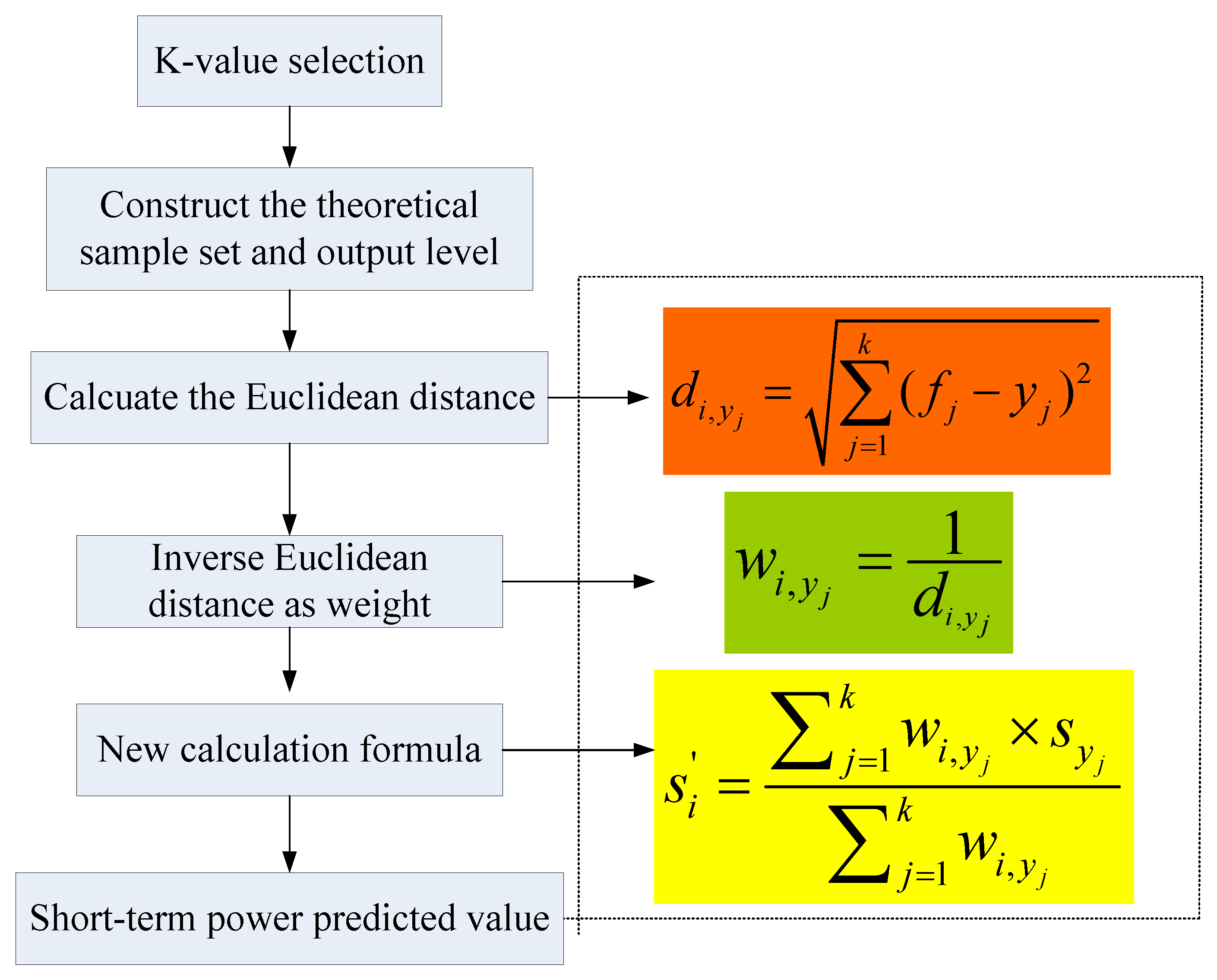
As mentioned above, the characteristics of the National Electricity Market (NEM, Australia) data set obviously reveal that a day can be regarded as a physiological cycle (the so-called micro-production cycle), and it can be divided into three stages: (1) the first stage, from 0:00 to 8:00; (2) the second stage, from 8:00 to 16:00; and (3) the third stage, from 16:00 to 0:00. The electricity load forecasting values in the third stage can be found by using the electricity load data from the first two stages, it also reflects the applicability and rationality of this model.

The BPNN model, also known as the back propagation neural network, which is, through the training of the sample data, to continuously revise the network weights and thresholds to reduce the forecasting errors along the negative gradient direction, and eventually approximate the expected output. BPNN model has been widely applied in function approximation, data compression, and time series forecasting. In order to reveal the self-adaptability and sensitivity of electricity demanding behavior, the BP neural training toolbox of the MATLAB software, R2017a version, was implemented to forecast electricity load values by using the data of the first two months (for the large sample), or using the data of the first three weeks (for the small sample). In the BPNN modeling process, network layers were chosen as three, and intermediate neurons were selected as 10. The functions for hidden layer and output layer function were chosen as follows: Tansig (Tangent S type transfer function) and Logsig (Logarithmic sigmoid transfer function) were used as the implicit layer node transfer function, and Trainglx function was selected as the output layer node transfer function. Then, the forecasting accuracy indexes for each sample were calculated for comparison.

The proposed W-K-NN model not only has several theoretical advantages, such as less training parameters and good timeliness, but also had higher forecasting accuracy than ARMA and BPNN models, for both the small sample and large sample, as shown in

Table 5. Comparison of four forecasting models for the small sample (RMSE, NMSE, MAE and MAPE). Unit: MW.

Forecasting Period	W-K-NN				K-NN				ARMA				BPNN
	RMSE	NMSE	MAE	MAPE (%)	RMSE	NMSE	MAE	MAPE (%)	RMSE	NMSE	MAE	MAPE (%)	RMSE	NMSE	MAE	MAPE (%)
Jan.	586.03	0.34	1.04	3.87	853.27	0.39	1.17	5.93	1007.1	0.38	1.31	15.21	2263.2	0.41	1.72	20.29
Feb.	342.29	0.64	1.22	3.50	367.07	0.08	1.66	5.71	977.34	0.55	1.23	13.95	2113.39	0.58	1.71	19.28
Mar.	636.97	0.30	0.98	3.58	1081.62	0.95	1.09	5.38	782.04	0.35	1.10	13.2	1712.83	0.57	1.34	16.88
Apr.	435.60	0.87	0.97	3.96	415.30	0.20	1.08	7.94	729.12	0.34	1.02	12.8	2429.68	0.46	1.85	23.09
May.	415.28	0.08	0.95	3.77	347.23	0.12	1.03	5.70	737.64	0.39	1.06	12.1	1260.25	0.95	1.11	12.88
Jun.	271.31	0.62	1.12	4.12	302.43	0.05	1.25	6.18	1026.18	0.48	1.47	14.86	3972.30	0.49	3.03	30.45
Jul.	585.92	0.34	0.92	3.93	571.71	0.32	1.03	5.99	752.94	0.47	1.07	11.13	1350.94	0.41	1.01	11.01
Aug.	825.47	0.64	0.88	3.74	1146.88	1.24	0.93	6.61	833.6	0.41	0.91	10.61	1411.80	0.58	1.17	13.45
Sep.	485.79	0.30	0.85	3.55	467.92	0.28	0.95	5.33	654.54	0.36	0.91	11.22	1395.50	0.57	1.15	13.89
Oct.	1,885.15	0.87	1.33	4.39	1917.09	0.90	1.48	6.96	1560	0.35	1.67	90.09	2972.63	0.46	2.04	78.82
Nov.	320.80	0.08	1.10	4.01	343.61	0.10	1.23	8.27	864.72	0.29	1.13	12.87	2355.56	0.95	1.59	17.58
Dec.	1106.39	0.62	1.01	3.68	1324.44	0.89	1.04	5.52	1240.3	0.33	1.08	14.01	1489.43	0.49	1.13	16.15

and

Table 6. Comparison of four forecasting models for the large sample (RMSE, NMSE, MAE and MAPE). Unit: MW.

Forecasting Period	W-K-NN				K-NN				ARMA				BPNN
	RMSE	NMSE	MAE	MAPE (%)	RMSE	NMSE	MAE	MAPE (%)	RMSE	NMSE	MAE	MAPE (%)	RMSE	NMSE	MAE	MAPE (%)
Mar.	857.63	0.46	1.03	4.37	868.63	0.48	1.42	8.02	1300.8	0.22	1.37	16.22	1793.77	0.22	1.44	16.67
Jun.	847.39	0.21	0.98	3.48	1433.48	0.56	1.45	7.33	1557.44	0.19	1.47	15.57	1199.19	0.09	1.00	10.58
Sep.	553.50	0.18	1.04	3.78	497.69	0.15	1.10	5.54	909.6	0.18	1.03	12.15	4885.83	3.39	3.84	43.06
Dec.	814.08	0.50	1.14	4.89	1148.63	0.99	1.15	9.57	1128.56	0.23	1.19	14.34	1708.64	0.23	1.41	16.21

, respectively. Thus, it is more suitable for solving the nonlinear problem with time-varying uncertainties in short-term load forecasting. The error values of RMSE and NMSE, obtained by the proposed W-K-NN model, in the small and large samples were both relatively small, and from Figure 3 and Figure 4, the stability of the proposed W-K-NN model had certain volatility. However, with the better performances of these two evaluation indexes, the proposed W-K-NN model could provide more accurate forecasting results. For ARMA model, its accuracy may be affected by different parameters, due to the assumptions of the ARMA model that even if all the errors are completely objective, the forecasting process will still be affected by some uncertainties. Thus, the forecasting errors were unable to be reduced. However, the stability of the forecasting errors of the ARMA model was better, which indicates that it has its own robustness and inherent regularity. For the BPNN model, not only were the forecasting errors large, but also the stability of the forecasting errors fluctuated largely. This may be caused by the lack of training set of the BPNN model. After the case comparison and empirical investigation, the specific reasons for the above situation were found as follows: (1) The summer vacation of Australian schools is often from the middle of November to the end of February; therefore, the electricity consumption demonstrates great differences and instabilities from December to January; (2) From the view point of the annual plan of industrial production, a large amount of industrial production is generally carried out at the beginning of the year. Principal marketing activities are carried out in the middle of the year, namely clearance of stock. Additionally, some output may be increased at the end of the year. Therefore, the differences of the electricity consumption are relatively large between the beginning and the end of a year, but the middle of the year is relatively stable.

Finally, verification of the significance of the accuracy improvement of the proposed W-K-NN model was also an important issue. The forecasting accuracy comparisons in both samples among ARMA, BPNN, and W-K-NN models were implemented by the Wilcoxon signed-rank test under 0.025 and 0.05 significant levels (one-tail), respectively [29,30]. The Wilcoxon signed-rank test is a famous statistical test tool. It is suitable for pair comparison to evaluate whether their performance is different. It often uses Student’s t-test as the statistics, particularly for those cases that the associate population could not be guaranteed to satisfy the normally distributed [31]. The Wilcoxon signed-rank test results for small and large samples are demonstrated in

Table 7. Wilcoxon signed-rank test for the small sample.

Compared Models	Wilcoxon Signed-Rank Test
	α = 0.025; W = 4	α = 0.05; W = 6
W-K-NN vs. K-NN	2 a	3 a
W-K-NN vs. ARMA	3 a	2 a
W-K-NN vs. BPNN	3 a	3 a

^a denotes that the W-K-NN model significantly outperforms other alternative models.

and

Table 8. Wilcoxon signed-rank test for the large sample.

Compared Models	Wilcoxon Signed-Rank Test
	α = 0.025; W = 4	α = 0.05; W = 6
W-K-NN vs. K-NN	3 a	3 a
W-K-NN vs. ARMA	3 a	2 a
W-K-NN vs. BPNN	2 a	2 a

^a denotes that the W-K-NN model significantly outperforms other alternative models.

, respectively. Obviously, the proposed models all received significant forecasting results, compared with other alternative models, under two significant levels.

In order to compare the advantages of the proposed model, a similar model (namely recency effect model) from a published paper [32] in GEFCom2012, was employed. The recency effect model was also used to extract similar features in time, the more prominent forecasting effect was reflected in summer and winter. According to [32], in summer, the electricity load data from June 1 to June 17, 2007 (17 days in total) were employed as the training set to forecast the electricity load from June 18 to June 24 (total 7 days); in winter, the electricity load data from October 21 to November 13, 2007 (24 days in total) to forecast the electricity load from November 14 to November 21, 2007 (total eight days).

The forecasting results of the proposed model are demonstrated in Figure 7. In which, it was found that the forecasting accuracy was superior at both the peak point and the valley period, particularly for the valley, its forecasting performances were very prominent.

Table 9. The forecasting errors of the proposed model.

Seasons	RMSE	NMSE	MAE	MAPE *
Summer	0.0759	0.555	5.50	3.74 (3.86)
Winter	0.0636	0.595	6.71	3.90 (3.86)

*: The MAPE is based on the hourly average error values; and the value inside of () is the average error value from the recency effect model.

shows the forecasting errors in terms of RMSE, NMSE, MAE, and MAPE. It can be seen that it had the same advantages and effects as the recency effect model. It was more prominent in summer, which indicates that it was superior in capturing the laws of summer economic activities.

5. Conclusions

In this paper, the nearest neighbor distance algorithm was adopted to give the appropriate weights for each data point to construct a new short-term load forecasting model (the so-called W-K-NN model), and this proposed model was then applied to the actual short-term load forecasting job. Some important conclusions were as follows:

(1)

Through the different samples verification and forecasting error analysis, it is found that the proposed W-K-NN model has higher forecasting accuracy and effectiveness. Additionally, it can be widely applied in short-term load production decision making, for example, power users can make efficient energy-saving renovation plans based on the evaluation results, and eventually improve the electricity efficiency.

(2)

Compared with the ARMA model and the BPNN model, the fitting ability of the proposed W-K-NN model is more superior to these other two models. It can not only objectively and comprehensively reflect the actual energy efficiency level of power users, but also better meet the development needs of modern smart grid and intelligent control systems.

(3)

In the future, authors will combine the short-term forecasting approach with the medium-short-term forecasting approach, to detect the market demand shrinking information problem, particularly for the upper-point point (peak) of the electric behavior regulations. Meanwhile, authors will also look for an optimized approach to optimize the weight, in order to improve the forecasting accuracy, for example, for the complete, the same, or very closed commodities, their weights would be set as huge or even infinite; therefore, when calculating the reciprocal distance, some constant can be added to revise the distance.