1. Introduction
During the last fifteen years, we have been progressing to a large deployment of power electronics with the goal of conducting non-linear loads in a frame of distributed energy resources at generation, transmission, and distribution stages. This fact, along with utilities deregulation, elicits the need for a new concept of power quality (PQ) that should affect standards and measurement equipment aligned with an effective operation system [
1,
2].
Indeed, one of the new challenges of PQ analyzers resides in the fact of registering new PQ events that have been arising in the smart grid (SG) and dramatically affect sensitive electronics. As a consequence, there is a special need for PQ monitoring analysis techniques that account for new disturbance assessment techniques. These not only detect the presence of anomalous power, but also allow adopting protection measures, which eventually enable the correct on/off load or mitigation strategies. In particular, the focus of new class C instruments is on the quasi steady condition, more specifically on waveform distortion (e.g., harmonic, inter-harmonic) [
2,
3,
4].
Depending on the situation being considered (e.g., type of disturbances, measurement campaign), different equipment can be used. In the frame of the current electrical network, harmonics are gaining attention, mainly due to their proliferation as a consequence of the non-linear loads in distributed energy resources (DERs). However, traditional harmonic and spectrum analyzers are mainly based on fast Fourier transform (FFT) (e.g., power spectrum) and may not register low-level (but persistent) harmonics or any other electrical disturbance. Certainly, a conventional disturbance monitor is useful for initial tests at the point under study, but it is difficult to extract the characteristics of a disturbance from the information available. Therefore, it is recommended to add new capabilities for a more detailed or specific analysis of a power quality issue [
4,
5].
The selection of the most appropriate implementation for a given digital signal processing (DSP) algorithm intending to build autonomous PQ measurement equipment is always an important decision, in order to meet the design objectives.
In general terms, a processor-based implementation gives the greatest design flexibility with the lowest design effort, but provides the lowest hardware exploitation and energy efficiency. On the other hand, a specifically manufactured device obtains the best hardware exploitation and energy efficiency, but requires a very high design effort with the lowest design flexibility.
Reconfigurable devices, and particularly field programmable gate arrays (FPGAs), have been considered since their introduction as a trade-off solution for the implementation of DSP algorithms. Consequently, many of the improvements in the technological capabilities and design tools have been targeted for this task, extending the use of FPGAs to application fields previously reserved to processors because of their required flexibility, or to specific hardware because of their high demanding performance.
These improvements have meant that typical DSP functions, like digital filtering or FFT, have an easy and straightforward implementation using FPGAs, with the provision of many adjustable hardware cores that can be used in a similar way to software functions in a processor program. Thus, the implementation of a complex DSP function in a FPGA can be considered as an affordable design task in many situations, enabling its inclusion in a real-time digital processing system as small and autonomous measurement equipment.
The spectral kurtosis (SK) is an example of a complex DSP function, of interest to the PQ field and whose implementation in a FPGA can be advantageous over a processor-based alternative. This function is a fourth order statistic estimator that can be considered as the frequency domain version of the statistical variance named kurtosis. It is a useful tool to indicate the presence of transients in a signal and their locations in the frequency domain. It also provides additional information with respect to second order quantities given by the power spectrum density. This information can be used to discriminate between constant amplitude harmonics, time-varying amplitude harmonics, and noise (see
Appendix A for more detailed information).
The SK has been used in several applications: (1) for detecting and removing radio frequency interference in radio astronomy data [
6], (2) for bearing fault detection in asynchronous machines [
7], and (3) for termite detection [
8], and PQ analysis can be improved by the use of this function in the diagnosis of presence of underlying electrical perturbations [
9].
The SK is calculated in all these contributions by means of a processor-based system using a specialized high-level language such as MATLABTM, Octave, SciPy Python’s library, etc., and involves the use of a general-purpose desktop computer. A laptop computer may be required depending on the location of the system under test.
This implementation is the most accurate when the objective is to demonstrate the capability of the algorithm to perform the desired analysis or detection task. However, when real-time operation capability, energy efficiency, equipment size, and many other practical characteristics of autonomous PQ measurement equipment are taken into account, an alternative implementation using FPGAs must be considered. The viability of this solution for the implementation of the SK has been shown in Reference [
10], but it makes no assessment of different implementation alternatives.
Comparative studies between FPGA and processor-based implementation of different algorithms can be found in many previous works. Specifically, it is quite common to find comparative implementations using FPGAs, common desktop processors, and graphics processing units (GPUs) [
11,
12,
13,
14,
15,
16]. These studies are oriented to show the advantages of using the so-called General Purpose Computing on GPUs’ paradigm. This paradigm was first introduced by NVIDIA Corporation in 2007 with its Compute Unified Device Architecture, an application programming interface that allows the use of a GPU for general purpose computing, exploiting the highly parallelized GPU hardware resources to implement non-graphic applications. These studies show that this is a very attractive alternative (probably the best one) if we are considering the use of a conventional computer equipped with a high-end graphics card. Although it could be a suitable implementation for easily accessible systems with unlimited power, it is not an option for autonomous measuring equipment, where power consumption and size are key aspects.
In this paper we present a performance evaluation of different implementations of the SK algorithm. Processor-based and FPGA-based implementations are compared, focusing on the ultimate goal of obtaining autonomous PQ measuring equipment.
2. Materials and Methods
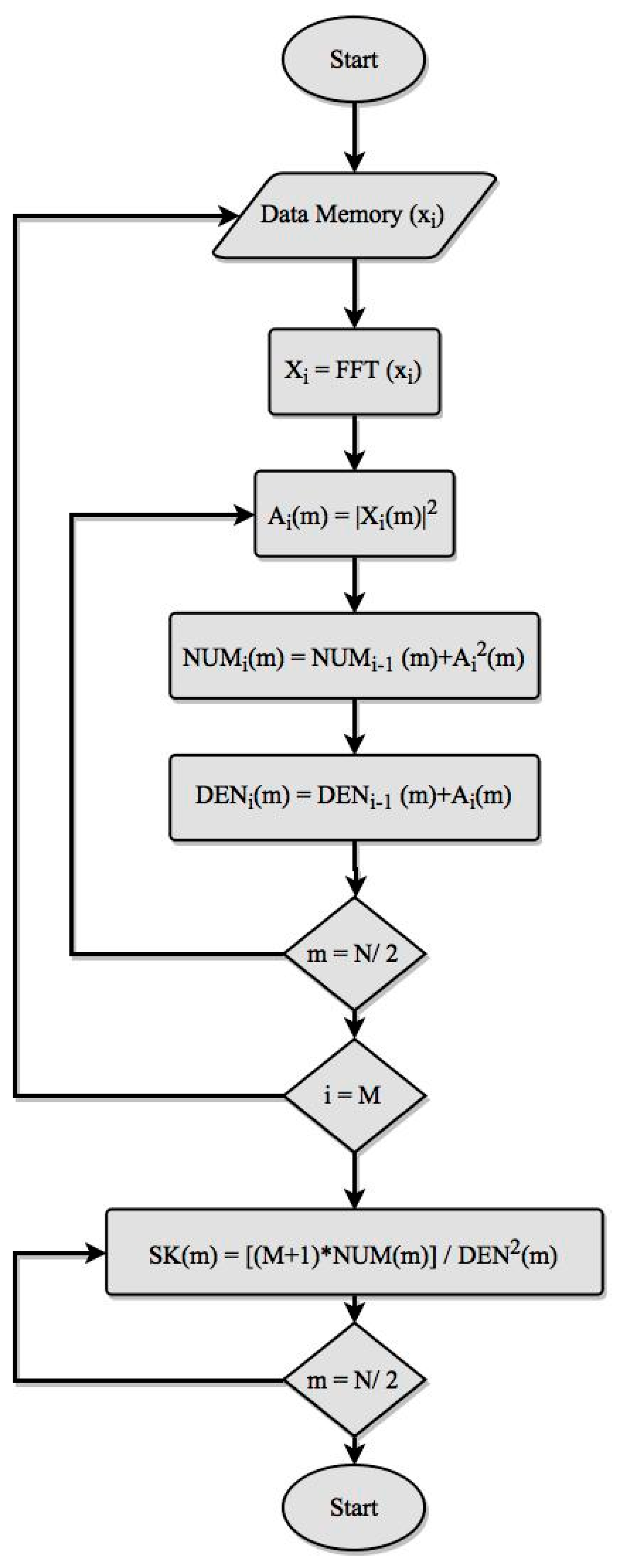
In order to establish a consistent comparison between the different implementations of the SK, explained in details in
Appendix A, the same basic flowchart is followed to evaluate Equation (A2). This flowchart is represented in
Figure 1.
The comparison only takes into account the evaluation of the SK, and it is assumed that data are available at the rate needed by the computational core (processor or FPGA). The relationship between data sampling frequency and computation will be analyzed in section Results.
The values of M, N, and input data width have been selected in order to obtain results with statistical validity, sufficient frequency, and amplitude resolution. Thus, values of M = 1000, N = 2048, and 16 bits of data width have been chosen.
The FFT function has been represented in the flowchart as a single step because it is available as a software function or as a hardware core.
The flowchart also includes two nested loops to evaluate the summation functions of the Equation (A2). The outer one was repeated M times (index i), one for each data frame, while the inner one is repeated N/2 times (index m), one for each frequency step (although data frames are N points length, the negative and symmetric spectrum of FFT has not be considered, as usual). From the summation of the functions evaluated for each frequency step, a final loop was executed N/2 times to evaluate the SK.
Since input data are acquired by means of an analog to digital converter (ADC), an integer format was applied to the input data. However, the mathematical treatment greatly increased the range of the intermediate values. Consequently, a conversion to floating point was performed, but it was not explicitly shown in the flowchart. Output data were obtained also in floating point format.
All the operations in the flowchart are represented sequentially, without taking into account that some of them can be executed concurrently.
2.1. FPGA Implementation
The FPGA version of the SK operator is built by means of the hardware description language VHDL. Only the synthesis subset of VHDL’93 is used to design the circuit [
17]. The hardware description was synthesized using the Xilinx Synthesis Tool, XST, which was included in Integrated Synthesis Environment, ISE 14.2 software suite provided by Xilinx
TM, which is the manufacturer of the chosen devices.
As it is intended to make a comparison from a practical point of view, some Intellectual Property (IP) cores from Xilinx were used in order to facilitate and speed up the design. This fact not only decreases the FPGA design cycle, but also ensures accurate results, since IP cores were verified and optimized.
The computation of the FFT was accomplished with one of these IP cores, and it was performed using integer format to avoid losing resolution [
18]. The output of this core was converted to floating-point format (as has been previously indicated) and mathematically processed. Both format conversion and mathematical process were implemented using floating point arithmetic IP cores [
19]. All IP cores were parameterized, requiring a previous setup process to adapt them to the SK algorithm design, allowing the specification of different design strategies and objectives. This feature is one of the main advantages of a FPGA implementation.
Although the processing was designed and implemented using Xilinx software tools and devices, the design was described in VHDL, and the logical resources and IP cores used in the implementation are commonly available Therefore, it can be adapted to other similar devices from others companies.
The circuit is divided into two main modules:
Making use of the previously mentioned adaptability of the IP cores, two versions of the SK FPGA implementation were designed and tested in order to achieve the best results in either performance or area. Additionally, both designs were implemented using two different FPGA series from Xilinx: Spartan6 and Artix-7, which are the lowest end series of the manufacturer. Particularly, the devices used are XC6LS16 and XC7A100T, housed in Digilent’s Nexys3 and Nexys4 evaluation boards, respectively.
To obtain the best results in terms of performance, the IP cores have to be setup for minimal latency, implying the use of a pipelined structure for the FFT [
18] that enables the use of a streaming input/output, i.e., a new set of data which can be read at the input while the previous one is still being processed.
Focusing on the use of resources, to obtain the best results in terms of using them, the IP cores have to be setup for maximal latency, implying the use of a conventional radix-2 structure for the FFT that needs the use of a burst input/output, i.e., it is necessary to completely process a set of data before reading a new one.
For IP cores other than FFT, the latency can also be adjusted, but a pipeline structure is always used [
19].
By combining the two-implementation setup with the two target devices, we obtained four different experiments,
Table 1.
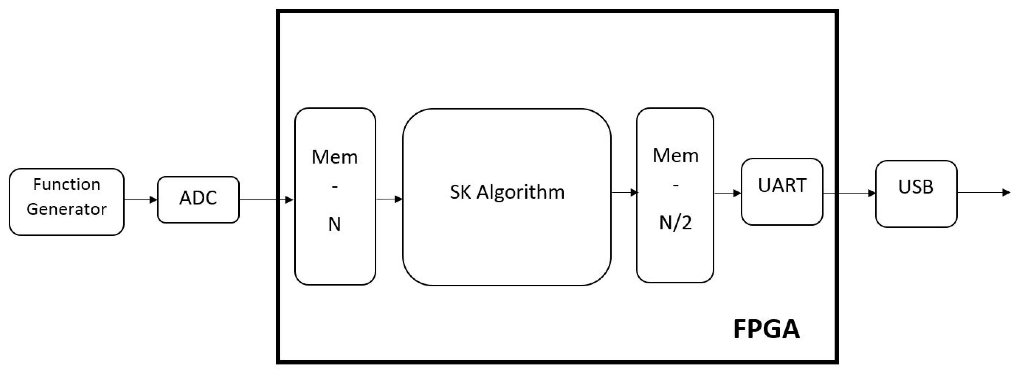
In order to test the implementations, some additional circuitry was added to the SK algorithm circuit, as shown in
Figure 2.
The FPGA takes its input from an external ADC that is connected to a function generator during the test process. The output of the SK evaluator is sent using an UART through an USB port in order to be analyzed and presented in a computer. The USB circuitry is part of the evaluation board.
To synchronize the ADC and the SK evaluator, an internal dual port memory stores the samples until a set is complete (N samples have been acquired). Then the SK evaluator computes the sample set without interrupting the sampling process.
From the M (1000) sets of N (2048) samples of input signal, the SK evaluator generates N/2 (1024) values corresponding to the SK value for each frequency step. These values are stored in an internal memory to synchronize the SK evaluator with the UART operation.
The SK evaluator receives the data in integer format and produces its results in floating point format, specifically in single-precision IEEE-754 format.
2.2. Processor-Based Implementation
The processor-based implementation is written in the Python programming language for the following reasons: (1) its scientific and numeric capabilities, which assure that the mathematical functions needed to build Equation (A2), such as FFT or floating-point arithmetic are available; (2) its portability, which guarantees that the code can be executed on platforms built around processors with different architectures; and (3) accessibility, which makes the results easily reproducible.
As the comparison is oriented to the implementation of autonomous measurement equipment, the processors used to execute and test the algorithm were selected from those that are typically used to build embedded systems. Specifically, an ARM Cortex-A7, an Intel Atom N270, and an Intel i7-3517U were selected. The first one is representative of the type of processors that can be found in systems like a Raspberry Pi, while the devices from Intel are in the low and high end of the processors used in industrial embedded computers from companies like Wordsworth.
Table 2 contains a summary of the characteristics of the processor-based implementations.
The experimental setup for the processor-based SK implementations was simpler than the corresponding setup for the FPGA implementations. This is because we were only interested in the evaluation of the SK algorithm. Therefore, the input test signal could be synthesized by the software instead of being acquired, and consequently, the ADC was not needed. Additionally, the results can also be represented using the same software that performs the SK algorithm.
2.3. Preliminary Test
Before any performance evaluation, all the implementations were tested to verify that their behavior was correct. Several types of signals were tested and the resulting SK in each case was the expected.
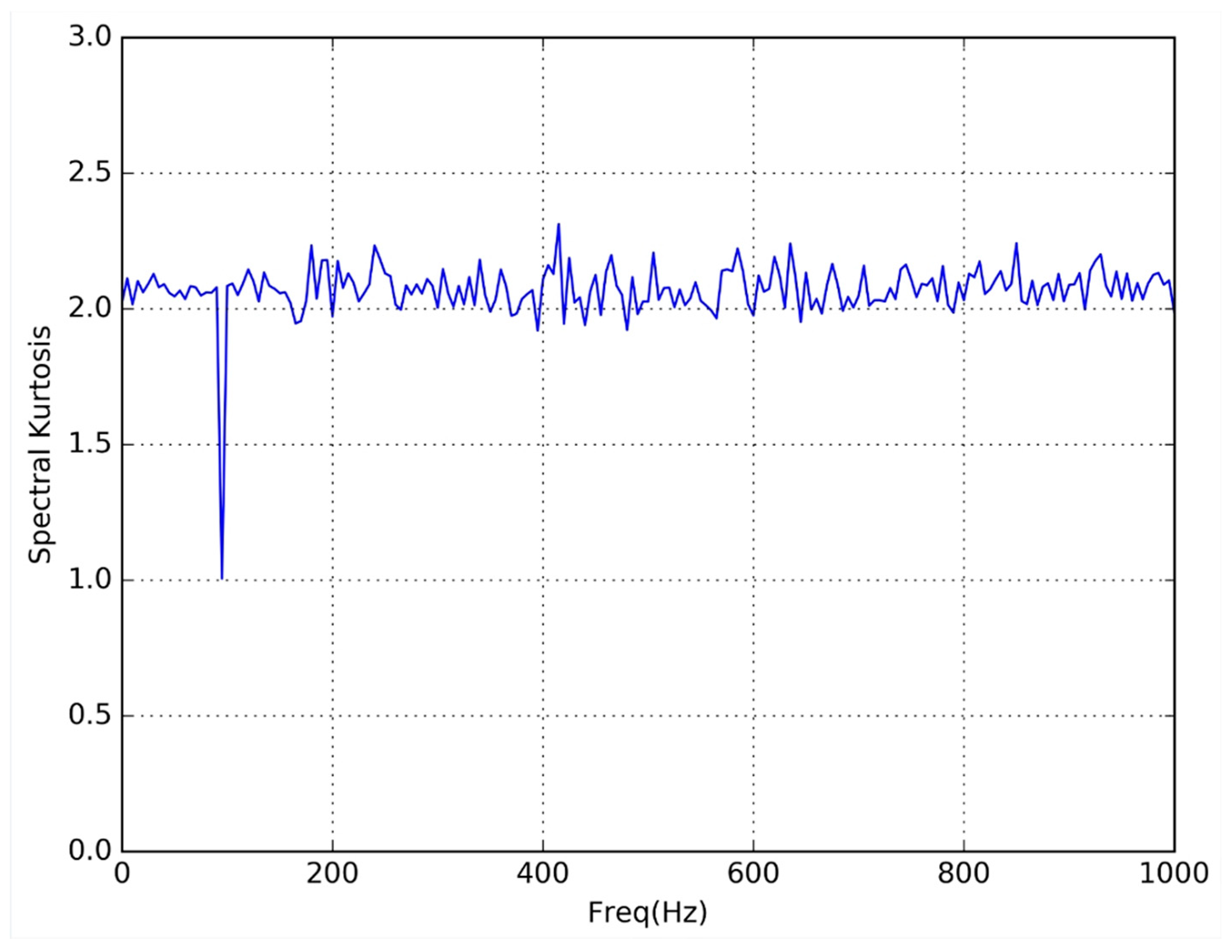
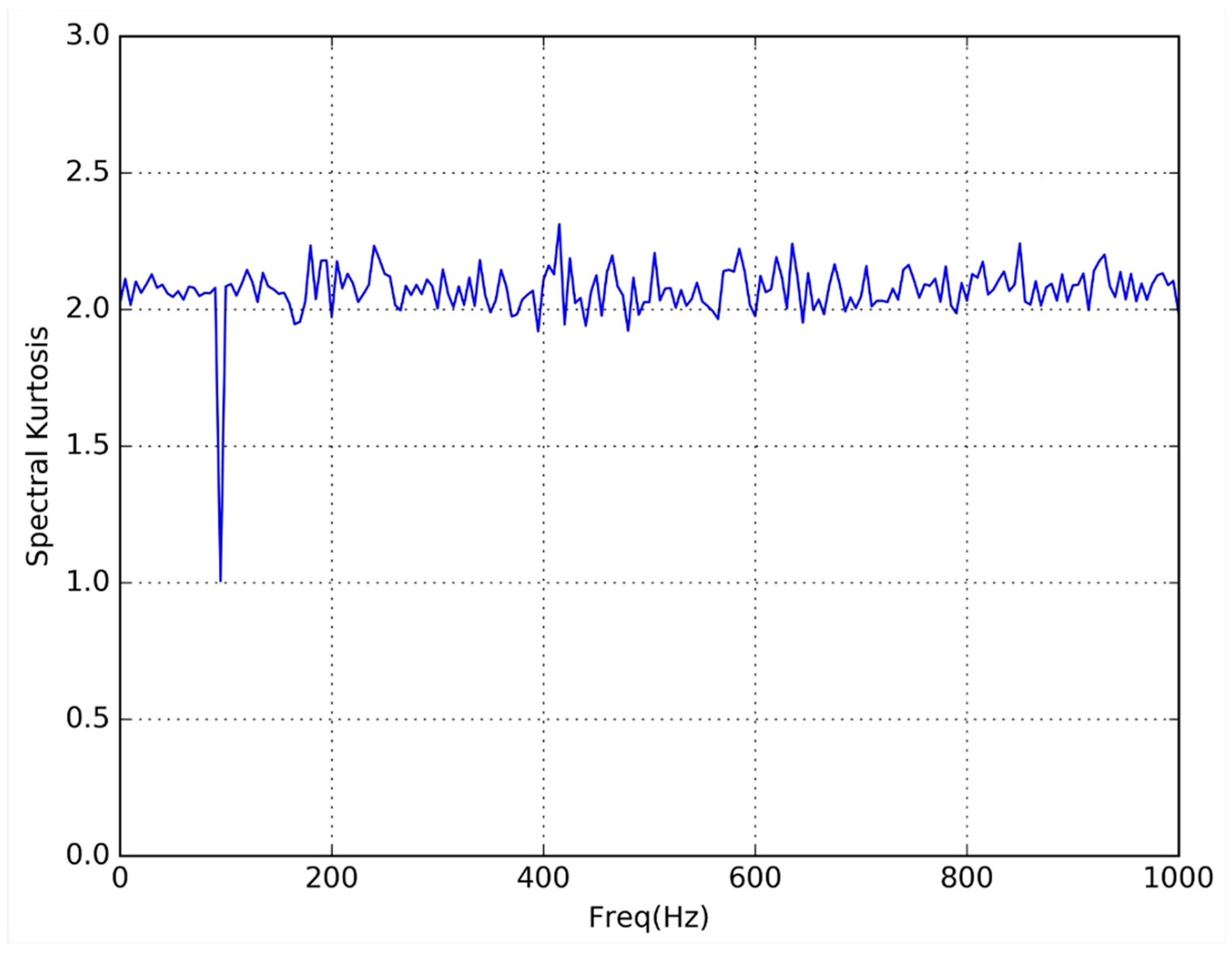
As a sample of this preliminary test,
Figure 3 and
Figure 4 respectively represent the SK obtained from experiments FPGA 1 and Processor 1. In both cases the input signal was a 100 Hz sine wave (the amplitude was not significant because the SK shows the variability of the harmonic content).
In both figures, the expected single spectral line (SK = 1) corresponding to the harmonic content at 100 Hz, can be seen. Also, the absence of harmonic content (SK = 2) for the rest of frequencies was visible.
As can be seen in the figures, the results obtained from the two types of implementation are exactly the same.
2.4. Performance Test
The main objective of this test was to compare the different implementations in terms of processing time. To evaluate this characteristic, input data was fed to the SK processing unit at the maximum possible rate. For the FPGA-based circuits, this condition was accomplished by passing the ADC and directly feeding the digital input. For the processor-based implementations, datasets were synthesized by software and stored in memory before the SK code was launched. This simulates the practical situation where data was available to the SK processor on demand, enabling the evaluation of the SK processing time.
One of the main differences that can be anticipated between FPGA and processor-based implementations is that processing time is constant for FPGA circuits but not for processor-based implementations. This is because the operating system is running onto the processor to arrange and distribute the processor time among different processes. Therefore, since the total processing time for the SK evaluator is essentially due to the repetition of the main loop in
Figure 1 M times, the best way to compare such different implementations is to divide the total time employed to complete the whole algorithm by
M, obtaining the averaged time needed to perform a single iteration.
For FPGA implementations, the measurement of this time was performed through the handshake signals of the different IP cores. These signals allow a direct monitoring of the computational process and are easily extracted from the FPGA.
For processor-based implementations, time measurement instructions have been included in the code to measure the elapsed time dedicated to solve the SK equation.
3. Results
3.1. Implementation Results for FPGAs
Although the main objective of the study is to compare the processing time, it is also of interest to show the cost in terms of used resources of the different FPGA implementations.
In general terms, to optimize timing results it is necessary to parallelize the implementation and, consequently, use a greater amount of hardware resources. The results represented in
Table 3 confirm this general assertion and quantifies it, showing that the time optimal implementation uses around a 60% more hardware resources than the area optimal circuit. This implies that the fastest version cannot be implemented in the smaller device.
The results of
Table 3 are divided into three different categories: Slices (Xilinx’s denomination for general purpose logic unit), block RAM, and DSP blocks. This is because the exhaustion of any of the three categories implies the impossibility of implementing the circuit, even if there are free resources in the other categories.
Table 3 also includes the maximum operating frequency for each implementation, a feature that will be very important to determine the time behavior of the circuits.
3.2. Preliminary Time Evaluation for FPGA-Based Implementations
One of the advantages of FPGA-based implementations is that their time behavior is mostly predictable. Their latency and maximum operating frequency can be evaluated from their structure, and this fact is exploited by the design tools that can offer very accurate time information.
While in this paper all the experimental results were measured, time predictions from design tools were used to elaborate extrapolations of the circuit behavior for different operating frequencies and implementation conditions. This is the reason this analysis was included.
Taking into account the flowchart of
Figure 1, two main parts can be distinguished in the evaluation of the SK. The first one performs the FFT and obtains the summations of Equation (A2), while the second one computes the product and division of this equation.
The first part is clearly more complex, and implies M iterations that run N/2 samples each, while the second part executes one single cycle that runs N/2 samples. Taking into account that M has to be large to give statistical validity to the results, it has to be concluded that the total execution time was expected to be almost proportional to M and completely dependent on the execution time of a single iteration of the first part of the flowchart.
For an FPGA-based implementation the FFT operation can be divided into three stages: data reading, processing, and result extraction. The first and the last stages use N clock cycles each, while the processing stage has a variable duration depending on the implementation parameters.
In any case, the evaluation of the squared terms and summations can be executed concurrently with FFT because this can be done as soon as data become available at the FFT module output, when result extraction stage begins. Therefore, the time needed to perform this evaluation was not added to the time required by the FFT, and only the longest one was used to determine the total execution time of one iteration.
The evaluation of the square terms and summations, as well as product and division, were always implemented by means of pipeline technique. Consequently, for each frame of data they used N/2 clock cycles.
For a pipelined structure the stages previously described for the FFT can be executed concurrently. Thus, at the same time a new set of data was being read, the results of the previous set were extracted, and different sets of data were processed simultaneously. The number of clock cycles to perform one FFT was therefore equal to N.
Nevertheless, for a radix-2 structure, the FFT stages were not concurrent and the number of clock cycles needed to complete the operation was greater than N. We have established experimentally a relationship between N and the number of clock cycles needed to complete the FFT. This relationship was obtained for 512 ≤ N ≤ 4096.
Table 4 shows the number of clock cycles needed to perform the different operations used in the SK evaluation for the different implementations as a function of
N.
The results in
Table 4 are valid for the intermediate iterations of the main loop in
Figure 1, which was repeated
M times. For the first and the last iteration the number of clock cycles can be greater because of the latency of the different blocks.
The latency for the evaluation of squared terms and summations had no effect because it was small (54 cycles max) compared to N/2, which was the number of cycles of the result extraction of the FFT that was not used (corresponding to the negative frequency spectrum).
Latency for the product and the division had little effect because this operation was performed only once at the end of the overall process.
Finally, the latency for the FFT was significant for the time optimal implementation only, because for the radix-2 implementation there was not concurrency. It was experimentally evaluated that the latency for the time optimal implementation of FFT (
LFFT) can be obtained from Equation (1).
Taking into account all of this information, the total processing time (
TSK) expressed in number of clock cycles can be evaluated using Equation (2) for an area optimal implementation, and using Equation (3) for a time optimal implementation, where
LP&D is the latency of the product and division operation, which is 40 cycles max.
For the usual values of
M and
N, these equations can be approximated by Equations (4) and (5), respectively.
3.3. Time Results
As it has been previously indicated, time results are presented in terms of the average time per iteration, which can be obtained dividing the total SK calculation time by
M. Assuming that the input data buffer is big enough, this quantity provides a good representation of the data processing capacity of the different implementations.
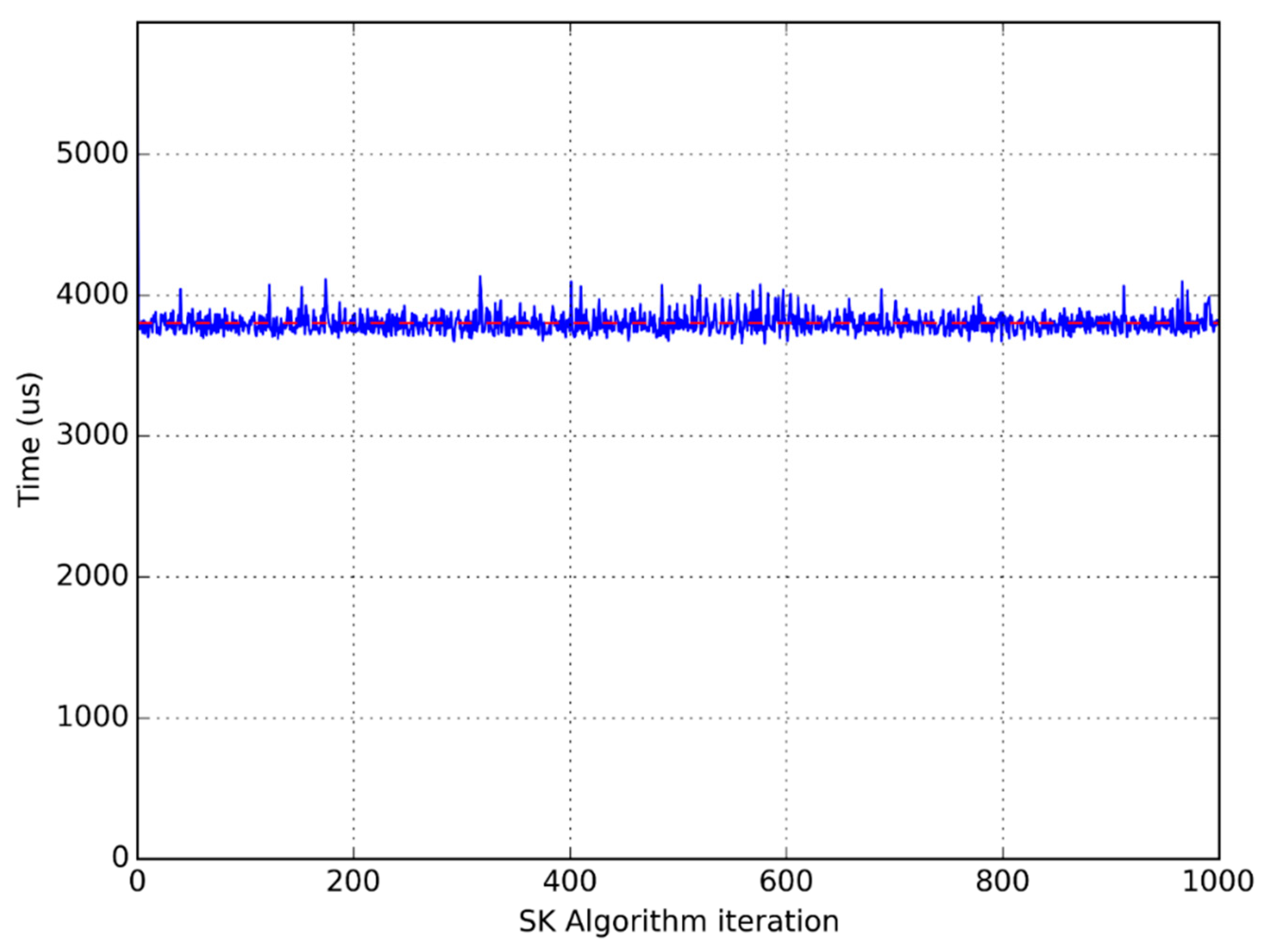
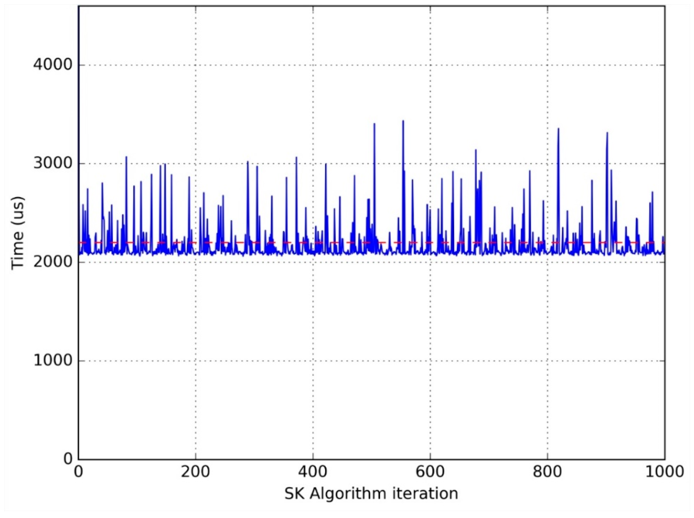
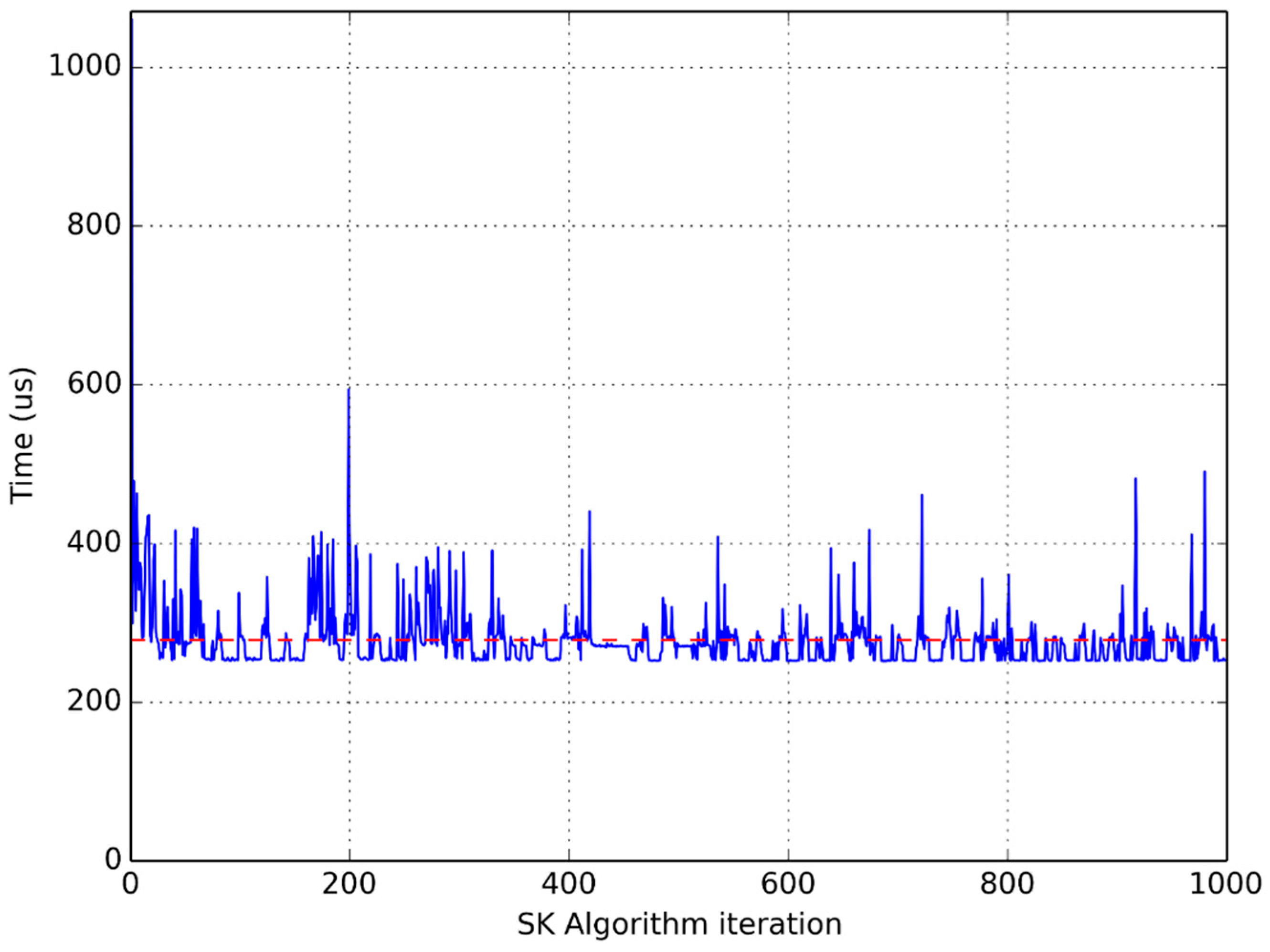
Figure 5,
Figure 6 and
Figure 7 show clearly the convenience of using this average time to compare different implementations. They are graphical representations of the time taken by each iteration of the main loop of the flowchart in
Figure 1. The horizontal dotted line represents the average time per iteration for each experiment.
It is clear that the time used to perform the same computation in the same processor greatly varies from one iteration to another, which advises the use of an average function to compare different implementations.
Also taking into account that the evaluated implementations are targeted to obtain autonomous PQ measurement equipment, it has to be assumed that input data to be processed are continuously acquired with a fixed sampling frequency.
The minimum value for this frequency is fixed by the characteristics of the signal to be acquired and it will be specific for each application. Consequently, it is not possible in a general study to select a particular value for this parameter, but it can be determined for each implementation which is the maximum value that can be reached. This value being a figure of merit that enables the comparison between different implementations.
The evaluation of the maximum sampling frequency that is compatible with a continuous data processing for each implementation, can be calculated by dividing the previously defined average time per iteration (Tcy,avg) by the number of samples that has to be acquired in this time (N).
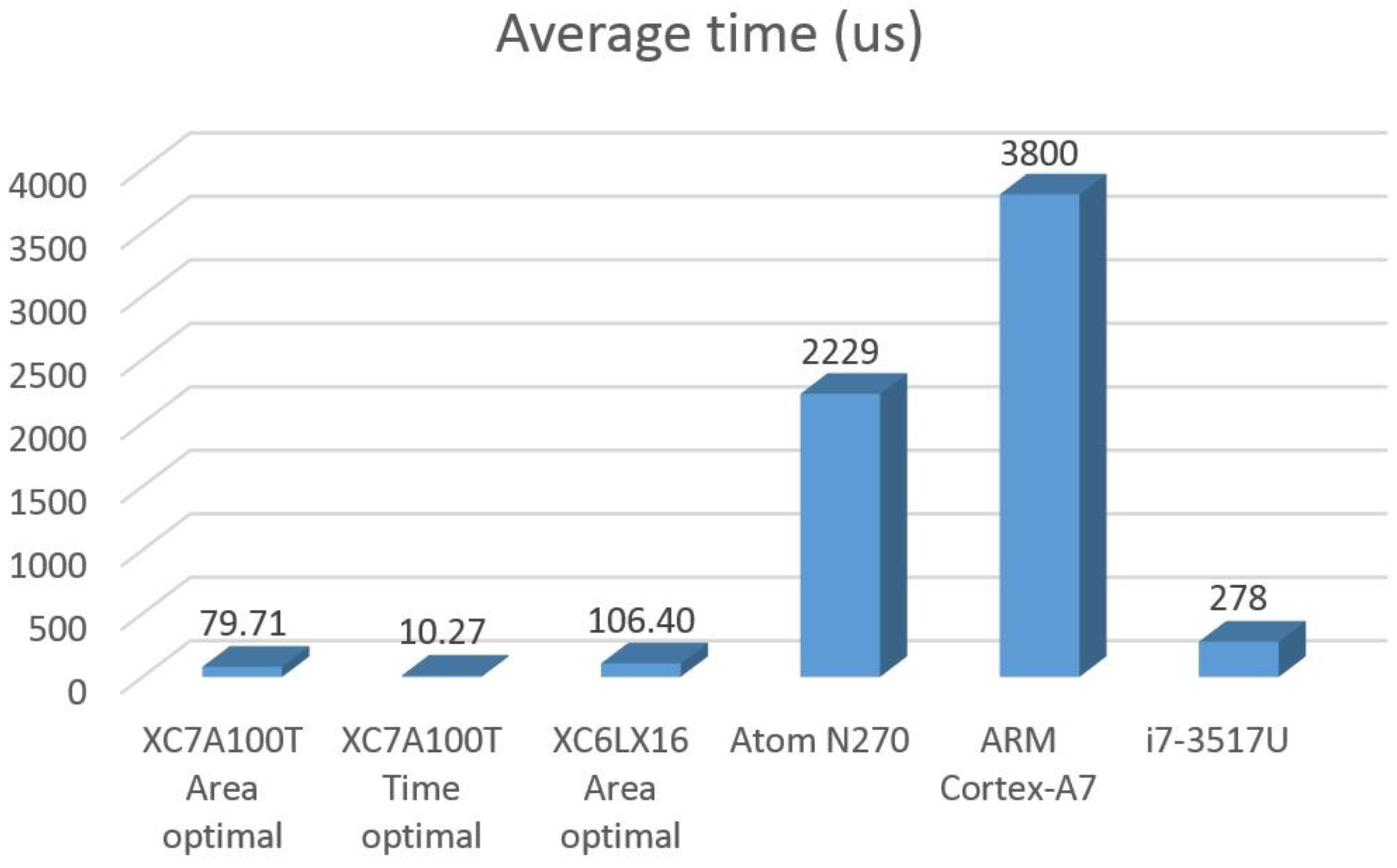
Table 5 summarizes the operating frequency (
fOp) regarding to all the implementations, the average time per iteration (
TIt,avg), which is graphically represented in
Figure 8, and the maximum data sampling frequency (
fS,max) that can be reached assuming a continuous data processing. In the last column of the table, a new parameter was included: the frequency exploitation factor (FEP), defined by de expression FEP =
fS,max/
fOp.
For instance, this factor shows that the worst FPGA implementation can reach the same processing capability as the best processor implementation with an operating frequency 33 times lower. It also shows that different FPGAs with the same implementation options are equivalent if they operate at the same frequency, revealing very similar hardware architectures.
4. Discussion
The main conclusion of the work is that an FPGA can be between 34 and 1740 times more frequency efficient than a processor for a typical SK function implementation. This implies that a lowest-end FPGA implementing a minimal resource use hardware structure (XC6LX16 area optimal) and with an operating frequency as relatively low as 60 MHz can reach a higher sampling frequency for a continuous processing than a high-end processor (i7-3517U) running at 1.9 GHz.
Performance results are not only better for FPGAs but also much more predictable and stable. This reduces the risk that the initial choice of an implementation does not fulfill the specifications when materialized.
Additionally, FPGA-based implementations can be tailored to different requirements, enabling the optimization of the solution to achieve diverse objectives. In this regard, it was shown that a time optimal implementation can reach a sampling frequency about eight times greater at the expense of an increase of 60% in the hardware resources used.
Despite this overwhelming result, processor-based implementations are still a reasonable option for low sampling frequencies, in the range of several hundred KHz for low-end processors, and up to several MHz for high-end processors, because of their ease of use and availability.
The experimental outcomes show that the FPGA technology processes the spectral kurtosis in a shorter time than general-purpose processors, even working at a lower frequency. This feature is accomplished even when low-cost models are used.
Since FPGAs and processors are made using CMOS technology, it can be assumed that most of the power consumption is dynamic and consequently, proportional to operation frequency.
The fact that two of the platforms used in this paper are laptop-based implies that we cannot include a quantitative evaluation of the power consumption, since a laptop incorporates many loads unrelated to processing. However, considering the proportional relationship between power consumption and working frequency, it can be concluded that FPGAs provide the best results in terms of power consumption. This is an additional advantage of using FPGA technology to develop autonomous PQ measurement equipment.

 ,
, 


