Abstract
In view of the complex calculation and limited fault tolerance capability of existing neutral point shift control algorithms, this paper studies the fault-tolerant control method for sub-module faults in modular multilevel converters on the basis of neutral point compound shift control strategy. In order to reduce the calculation complexity of shift parameters in the traditional strategy and simplify its implementation, an improved AC side phase voltage vector reconstruction method is proposed, achieving online real-time calculation of the modulation wave adjustment parameters of each phase required for fault-tolerant control. Based on this, a neutral point DC side shift control method is proposed to further improve the fault tolerance capability of the modular multilevel converter (MMC) system by compensating the fault phase voltage with non-fault phase voltage. By means of the compound shift control strategy of the DC side and AC side of the neutral point, an optimal neutral point position is selected to ensure that the MMC system output line voltage is symmetrical and the amplitude is as large as possible after fault-tolerant control. Finally, the effectiveness and feasibility of the proposed control strategy are verified by simulation and low-power MMC experimental system testing.
1. Introduction
In recent years, modular multilevel converters (MMCs) have found wide applications in the fields of medium and high voltage DC transmission, traction power supply, and high power AC drive, owing to their advantages of small output harmonics, high modularity and flexible structure. However, compared with the traditional multilevel converter, the MMC main circuit has more sub-modules (SMs) and contains more devices. Also, the control method is more complicated, and the fault probability of each SM and its internal devices increases accordingly [1,2]. If the SM faults in the system are not handled in time, there will be large deviations in the fault SM voltage, causing overload of other devices or SMs in the system. Thus, the non-fault phase may be impacted, and the overall output performance of the system will be affected [3,4,5]. Therefore, the fault-tolerant control after SM fault is of great importance.
Currently, the SM fault-tolerant control method for MMC falls into two major categories: redundant backup and non-redundant backup. Redundant backup control improves the operating characteristics of the system mainly by adding a backup SM to the bridge arms of each phase. When a fault occurs, a backup SM will function to ensure the continuous operation of the system. Despite the advantages of small loss and simple control [6,7], its disadvantages are also obvious. (i) After the fault, it takes a fairly long time to charge the backup SM and the output voltage waveform distortion is quite large [8,9]. (ii) The backup SM increases the cost of the converter [10]. (iii) In the same bridge arm, fault tolerance can be performed only when there are fewer faulty SMs than backup SMs [11]. In contrast, non-redundant backup control [12,13,14] requires no redundant SM. By use of the characteristics of the MMC’s topology and modulation strategy after SM faults occur, the system can operate at rated or reduced power by adjusting the control strategy. So far, the research on MMC non-redundant backup SM fault-tolerant control strategies has focused on energy balance strategy [15], zero-sequence voltage injection method [16] and neutral point shift control strategy [17]. Among them, neutral point shift control has a more obvious fault-tolerant effect. The traditional method is neutral point AC side shift control, that is, in case of asymmetrical maximum output power of the three-phase voltage after converter fault, the original neutral point is shifted to reconstruct an AC side phase voltage vector so as to obtain the adjustment parameters of the corresponding vectors (such as the amplitude and initial phase) and achieve symmetrical output of the line voltage. The related algorithm is complex and computationally intensive in this method. For the reconstruction of adjustment parameters, they first need to be stored after offline calculation and then obtained after table look-up for fault-tolerance. Originally used in the converter system of unit cascade topology, it is not fully applicable to the MMC system. In view of this, Ref. [18] proposed a control strategy for neutral point shift in the direction of the AC side fault phase voltage vector. Fault-tolerant control of SM faults in MMC systems is realized by optimizing the reconstruction of the AC side phase voltage vector and obtaining the algorithm of adjustment parameters. However, this method is not without problems. For example, the reconstruction adjustment algorithm is not simple enough, and there are restrictions on the number of faulty SMs. Also, the fault-tolerant capability is limited, and it is only applicable to SM faults in single-phase bridge arms.
This paper proposes an SM fault-tolerant control strategy based on neutral point compound shift for the MMC system under Phase Disposition PWM (PDPWM) [19], in hope of solving the problems of complex calculation and limited fault tolerance capability of existing neutral point shift control algorithms. Compared with the current approaches, it has three main benefits: (i) The computational complexity of the fault-tolerant reconstruction adjustment parameters is reduced, and the implementation of the algorithm is simplified by optimizing AC side phase voltage vector reconstruction method; (ii) The proposed neutral point DC side shift control method further increases the number of single-arm faulty SMs that can be fault-tolerant, and improves the fault compatibility; (iii) The optimal neutral point position can be selected based on the compound shift control mechanism of the neutral point DC side and AC side so that the MMC system output line voltage is symmetrical and the amplitude is as large as possible. Finally, the effectiveness of the proposed strategy is verified by simulations and experiments.
2. MMC Basic Principles and Fault Tolerance Capability Analysis
2.1. MMC Basic Principles
The MMC main circuit and its sub-module topology are shown in Figure 1. is the system DC bus voltage. Each phase consists of upper and lower bridge arms, in which two identical electric reactors () are connected in series. The reactors are intended to suppress the charging current at startup, restrain the internal circular current during operation, and reduce the rising rate of current when a fault occurs. Each bridge arm is connected in series with N SMs, and a single phase has a total of 2N SMs. Each SM consists of an upper and a lower switching tube (T1 and T2) connected in parallel with the capacitor C. On the left side of the converter is the DC side input end, and the midpoint where the upper and lower arm reactors of each phase are connected is the output end of the AC side. Due to the modular structure of the MMC, the number of SMs can be increased or decreased to meet the needs of different voltage and power levels.
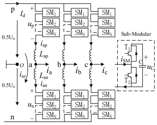
Figure 1.
Modular multilevel converter (MMC) main circuit and its sub-modular structure.
In each SM, the output voltage can be made zero or the capacitor voltage by controlling the status of the switching tubes T1 and T2. Since the SMs are independent of each other, the multi-level voltages can be output by continuously changing the number of input SMs of each bridge arm and superimposing them with appropriate basic modulation strategies.
2.2. Fault Tolerance Capability Analysis of MMC Bridge Arms under PDPWM Modulation
When the MMC system operates under PDPWM modulation, we first calculate the number of SMs that need to be input at each moment. Then, in combining the current direction of the bridge arm, the input SM is selected by means of the capacitor voltage sorting algorithm to ensure capacitor voltage equalization of each SM during system operation [19]. For the convenience of description, we take the SM open-circuit fault in the upper arm of a-phase as an example (N = 4) and discuss the fault tolerance capability of single-phase bridge arms.
Figure 2a,b show the SM modulation waves of the upper and lower arms and the corresponding output phase voltages in normal operation and in fault operation. It can be seen from Figure 2a that at the maximum modulation ratio, the output phase voltage amplitude can be as large as in normal system operation. According to Figure 2b, after SM fault, the a-phase upper arm modulation wave is derated to the middle area, and the total modulation area of the upper arm is divided into three parts: “modulation area”, “fault area” and “no modulation wave area”. The presence of “modulation area” is a necessary condition for the generation of modulation waves. Meanwhile, to ensure the symmetry of the output phase voltage and keep the total number of upper and lower arms constant, it is necessary to derate the modulation wave of the lower arm accordingly. At this time, the total modulation area of the lower arm is also divided into three areas: “modulation area”, “no modulation wave area” and “waste area”, and the maximum output phase voltage amplitude falls to .
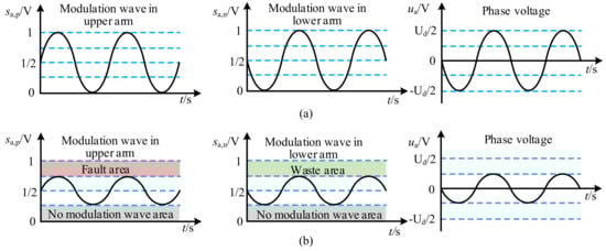
Figure 2.
Diagram of MMC fault tolerance capability analysis. (a) Normal operation; (b) Fault operation.
From the above analysis, it can be seen that to ensure a certain “modulation area”, the maximum number of faulty SMs allowed for the a-phase single arm is 1 when N = 4. Similarly, the method is also applicable to the fault tolerance analysis of b-phase and c-phase single arm in fault operation. Further analysis shows that when there are and faulty SMs in the upper and lower arms in any phase, the maximum number of faulty SMs for the fault phase single arm and the maximum output phase voltage amplitude are expressed as
Since the power device in SMs such as IGBT must not be on for a long time, the maximum number of faulty SMs allowed per bridge arm in any phase of MMC is , under the condition that the phase voltage is not zero. It can be seen that the allowed maximum number of faulty SMs in each phase under PDPWM modulation is limited. To further enhance the fault tolerance capability of all phases, the existing neutral point shift control strategy needs to be improved.
3. MMC Fault-Tolerant Control Strategy Based on Neutral Point Compound Shift
3.1. Improved Neutral Point AC Side Shift Control Strategy
Compared with the existing methods, the improved neutral point AC side shift control strategy is not only applicable to the MMC system, but also more convenient to reconstruct the output phase voltage vector after SM fault. Also, the phase voltage modulation wave reconstruction parameters required for fault-tolerant control can be obtained quickly. Here is the analysis of the main principle.
When the MMC system is in normal operation, the modulation wave signals of the upper and lower bridge arms of each phase are expressed in Equation (3).
where and () are the modulation waves of the upper and lower bridge arms of a, b, and c phases, is the initial phase of the three-phase modulation wave, is the modulation ratio of the system in normal operation, and is the angular frequency of the system output voltage. For the convenience of description, we assume that in normal system operation and are equal to 0, and , respectively. At this time, the phase voltages of a, b, and c are symmetric outputs under PDPWM modulation. The amplitude is the same, and the initial phase differs by sequentially. Shown in Figure 3a is the MMC output phase voltage vector diagram, where () is the output phase voltage vector in normal operation, and are the initial phase differences of the output voltage of adjacent phases.
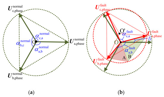
Figure 3.
The vector diagram of output phase voltages. (a) Normal operation; (b) Fault-tolerant operation.
When SM faults occur, the fault phase voltage output capability decreases as the number of faulty SMs increases. In order to keep the output line voltage of the system symmetrical and the amplitude as large as possible after the fault, it is necessary to reconstruct the original phase voltage modulation waves within the range of the output capability of each phase voltage. In other words, by adjusting the modulation ratio and initial phase of the modulation waves of each phase, we achieve stable fault-tolerant operations of the MMC system.
According to the neutral point AC side shift control principle, the reconstruction of the modulation waves of each phase voltage after the SM fault is essentially the vector reconstruction process of corresponding MMC output phase voltages. That is to say, after the fault, the phase voltage vector amplitude is adjusted according to the maximum output capability of each phase first, and then the initial phase is adjusted in such way as to reconstruct a phase voltage vector triangle with the largest symmetrical line voltage of the output amplitude. The improved neutral point AC side shift control strategy proposed in this paper aims to optimize the vector reconstruction method of the MMC system output phase voltage after SM fault and simplify the calculations of corresponding adjustment parameters to reduce the complexity of algorithm implementation.
Without loss of generality, we take the open circuit fault of a and b phases as an example to describe how the improved control strategy works. As shown in Figure 3b, the red marked () is the three-phase output voltage vector after fault-tolerant reconstruction, and its amplitude and initial phase have been adjusted. At this time, the initial phase difference between the output voltage of adjacent phases is , respectively, and indicates the initial phase change before and after the fault of a-phase voltage. Meanwhile, the equivalent neutral point of the output phase voltage vector triangle after reconstruction is shifted from the normal point O to O’. Then, the phase voltage amplitude output area will be shown as the red circle in dotted lines in Figure 3b. Correspondingly, using the improved control strategy proposed in this paper to reconstruct the modulation waves of each phase voltage after fault mainly involves a few aspects.
(1) Calculate and determine the maximum output voltage of each phase
First, calculate the amplitude of the maximum output voltage of each phase after fault according to Equation (2). In order to ensure the ability of the system to output symmetrical line voltages, the amplitudes of the three output phase voltages should be able to form an equilateral triangle. That is to say, the sum of the amplitudes of any two voltages should be greater than or equal to the amplitude of the output voltage of the third phase. If the condition is not satisfied, we select the maximum amplitude among the three output phase voltages, and denote the corresponding phase as k (). Then, modify the amplitude of the maximum output voltage that k phase is capable of, so that it is equal to the sum of the amplitudes of the maximum output voltages of other two phases.
where , , and .
After normalizing the amplitude of the maximum output voltage of each phase, we can obtain the maximum modulation ratio that each output phase voltage can be capable of.
where .
(2) Calculate and determine the initial phase of the output voltage vector of each phase
As shown in Figure 3b, make an auxiliary regular triangle A with as one side, and another side of triangle A and form another auxiliary triangle B. It can be deduced mathematically that the lengths of the three sides of triangle B are equal to , , and . Then, the initial phase difference can be obtained by using the cosine theorem.
Similarly, we can calculate and .
According to the amplitude and phase difference of the voltage vectors of any two adjacent phases, the line voltage amplitude after fault reconstruction can be obtained by applying the cosine theorem. Given , and , we have
According to the sinusoidal theorem, the change of initial phase of a-phase voltage after fault, and the initial phase of the three-phase output voltage vector after fault reconstruction can be expressed as the following equations.
where is the initial phase of three-phase output voltage vector after fault reconstruction ().
(3) Determine the modulation wave of the bridge arm voltage of each phase after fault
According to the calculated maximum modulation ratio and initial phase of the output phase voltage of each phase after fault, the modulation waves of the upper and lower arm voltage of each phase after reconstruction can be expressed as
where and are the upper and lower arm voltage modulation waves after reconstruction, respectively, .
It can be seen that after SM open circuit fault occurs in the MMC system, the implementation of the above control algorithm is basically a three-step process. First, the faulty SMs are bypassed according to the fault signal. Then, using the improved neutral point AC side shift algorithm, the phase voltage vector reconstruction adjustment parameters of the corresponding faults are calculated online. Finally, the original phase voltage modulation waves are reconstructed by use of the obtained adjustment parameters to generate new modulation wave signals.
Obviously, the above algorithm is simple and real-time, which reduces the complexity of the implementation considerably. However, there is still a problem that the fault tolerance capability of each phase is limited. If the number of faulty SMs of each phase exceeds a certain value, the system cannot continue to function. Therefore, we present a control method based on the neutral point DC side shift, which uses non-fault phase voltage to compensate for the fault phase voltage and thus improves its modulation area and fault tolerance capability. And combined with the improved AC side shift strategy, a neutral point compound shift control method is proposed to achieve optimal fault-tolerant control of MMC.
3.2. Neutral Point Compound Shift Control Strategy
3.2.1. Principle of Neutral Point DC Side Shift
From the MMC fault tolerance capability analysis under PDPWM modulation, it can be seen that whether the fault phase still has the ability to output phase voltage is affected by the “modulation area”. Here, we take the SM open-circuit fault in the upper arm of a-phase as an example (N = 4) and discuss the principle and advantage of neutral point DC side shift.
As shown in Figure 4a, when the number of faulty SMs is 1, if the neutral point DC side shift control strategy is adopted to shift the modulation waves of the upper and lower arms in the opposite direction on the DC side, the “waste area” and “no modulation wave area” after fault can be fully utilized to increase the “modulation area”. According to Figure 2b, it can be seen that after the use of neutral point DC side shift control, the amplitude of maximum output phase voltage can be increased from to . Apparently, neutral point DC side shift control can improve the faulty phase voltage output capability effectively.

Figure 4.
The diagram of neutral point DC side shift after sub-module (SM) fault in the upper arm of a-phase (N = 4). (a) One-fault operation; (b) Two-fault operation.
As shown in Figure 4b, when the number of faulty SMs increases to 2, if the neutral point DC-side shift control is not used, . Then the fault phase has no “modulation area”, and the system cannot continue to operate. After the neutral point DC side shift control is adopted, the fault phase still has phase voltage output capability, and the amplitude of maximum output phase voltage can reach . Obviously, the neutral point DC side shift control can improve the fault tolerance capability of the system effectively.
It can be seen that by using the neutral point DC side shift control strategy, the maximum number of faulty SMs allowed per bridge arm increases from to . The control strategy can improve the voltage output capability of the fault phase by increasing its “modulation area”, thereby improving the fault tolerance capability of the system.
3.2.2. The Implementation of Neutral Point DC Side Shift Control
For the three-phase MMC, the neutral point DC side shift must be performed simultaneously in the three phases. Therefore, when the fault state of each SM in the MMC is known, three-phase fault information should be comprehensively considered overall to obtain the final shift distance. The structure of the specific implementation process is shown in Figure 5, which mainly includes a fault number count module, a single-phase fault information fusion module, and a three-phase fault information fusion module.
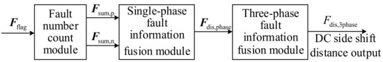
Figure 5.
The implementation process of neutral point DC side shift control.
It can be seen from the above figure that when the SM fault status is known, the neutral point DC side shift control method first uses the fault number count module to count the number of faulty SMs in the upper and lower arms of each phase. Then, the single-phase fault information fusion module performs fusion control on the fault information of the upper and lower arms, so that the shift distance satisfies the modulation area of the upper and lower arms at the same time. Finally, the three-phase fault information fusion module is used for fusion control so that the three-phase output voltages would have the same reference point to obtain the final neutral point DC side shift distance. The control principle and implementation method of each module will be described below.
(1) Fault number count module
Assume that the fault status of each sub-module in the MMC is known, and the fault status of all SMs in the three-phase arm is saved in the form of a matrix. We use N to represent the number of SMs of each arm, and “0” in the matrix indicates that the SM is working normally while “1” indicates the SM is faulty. For N = 4, the fault flag matrix is as follows when the system works normally.
In the above matrix, the three rows from top to bottom represents the three phases a, b, and c of the MMC, and each column from left to right represents the 1st to the 2N-th SM of each phase.
After the fault flag matrix is obtained, the total number of faulty SMs of each arm can be calculated easily by using the fault number count module. If the matrixes of and are set to store the number of faulty SMs in the upper and lower arms of each phase respectively, and the matrixes of and are set to logically calculate the fault information in the upper and lower arms of each bridge arm, then the and can be obtained by Equation (12).
(2) Single-phase fault information fusion module
For the single-phase circuit of normal MMC, the number of SMs in the upper and lower arms is symmetrical. If the SM fault occurs in the upper or lower arms, a decrease in the number of SMs that can be available to put into operation on one side means that the neutral point of the DC side needs to be shifted to the other side. Therefore, the determination of the neutral point shift distance and shift direction requires comprehensive consideration of the fault information of the upper and lower arms. Figure 6 shows the fault information fusion of a single-phase bridge arm when one SM of the upper and lower arms each is open circuit fault (N = 4). In the figure, the “fault area” corresponds to “1” in the fault flag matrix, and the “modulation area” corresponds to “0” in the fault flag matrix. That is to say, the corresponding single-phase fault flag matrix in this case is [1 0 0 0 0 0 0 1].
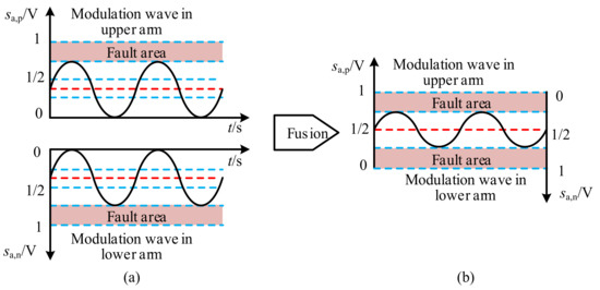
Figure 6.
The fault information fusion of a single-phase bridge arm (N = 4). (a) Modulation wave before single-phase fusion; (b) Modulation wave after single-phase fusion.
As can be seen from Figure 6a, the red dotted lines represent the positions of the DC side midpoint of the upper and lower arms when they are analyzed separately. At this time, the “modulation area” of both the upper and lower arms can be increased by the neutral point DC side shift. Since the DC side shift of the neutral point of any bridge arm must be shifted in the opposite direction to that of the symmetrical arm, the shift distances of the upper and lower arms are offset by each other in this case. The neutral point of the DC side should remain unchanged from the original position, and the shift distance is zero. Therefore, the modulation wave will be as shown in Figure 6b when the upper and lower arm fault information is fused to the same arm.
In order to realize the above-mentioned single-phase arm fault information fusion control, the logical “AND” operation can be performed on the upper and lower arm fault status, based on the results of which to obtain the neutral point DC side shift distance for the single phase. We set a matrix of to store the neutral point DC side shift distance of each phase, and a matrix of is set to realize the logical “AND” calculation of phases of the upper and lower arm fault status and the solution of the neutral point DC side shift distance. If the modulation wave direction of the upper arm is taken as the positive direction, after normalization we have
(3) Three-phase fault information fusion module
For the entire MMC system, when the fault information of the three-phase arm is different, the solutions of the neutral point shift distance of three phases in the matrix are different values. However, in order to make the output line voltage symmetrical, the shift distance needs to be consistent in the three phases. Therefore, on the basis of the single-phase upper and lower arm fault information fusion, three-phase fault information fusion should be conducted.
In order to facilitate the fusion of the three-phase fault information, the above fault flag matrix needs to be modified first. By shifting the SMs which are labeled “1” in the matrix to the front or the end of corresponding rows, the corresponding matrix is expressed as

Then, a logical “OR” operation is performed between the rows of the matrix to obtain a fault flag after the three-phase fault information fusion, and the operation results are stored in the matrix of . The operation method is shown in Equation (15), in which the first line , the second line and the third line in the matrix correspond to the three-phase fault flag, respectively.
After normalization, the three-phase neutral point shift distance can be obtained.
The following is an example of N = 4, one SM fault on the a-phase upper arm, two SM faults on the b-phase upper arm, and one SM fault on the c-phase lower arm. The three-phase fault information fusion results are shown in Figure 7. Figure 7a is the schematic diagram of modulation waves of each phase after single-phase information fusion. Although the modulation area of each phase is increased significantly, the DC side shift distance of the modulation wave obtained by single-phase information fusion alone cannot guarantee the consistent position of the three-phase DC side neutral point. Figure 7b is the schematic diagram of the “modulation area” after three-phase fault information fusion. As is shown, the final position of the three-phase neutral point should take the midpoint of the area, as indicated by the red dotted line in the figure. Consequently, after the three-phase fault information fusion and the calculation of three-phase neutral point shift distance, the final three-phase modulation wave is obtained as in Figure 7c.

Figure 7.
The fault information fusion of a three-phase bridge arm (N = 4). (a) Three-phase modulation wave after single-phase fusion; (b) Modulation area; (c) Three-phase modulation wave after three-phase fusion.
Obviously, when different numbers of faulty SMs occur in the MMC system, the above implementation method of neutral point DC side shift control is invariably applicable. Based on the method, the neutral point shift distance when the three-phase modulation area is satisfied simultaneously can be calculated.
According to the above analysis, it can be seen that the neutral point DC side shift control strategy can effectively improve the fault phase voltage modulation area, increase the possibility of AC side reconstruction after fault, thus enhancing the fault tolerance capability of the system.
3.2.3. AC Side Phase Voltage Vector Reconstruction Control under DC Side Shift
Neutral point DC side shift can provide more reconstruction space for the fault phase. In order to control SM fault-tolerant operation more effectively, it is still necessary to further reconstruct the phase voltage vector triangle after fault by combining the improved neutral point AC side shift control strategy described in Section 3.1. For this reason, the AC side phase voltage vector reconstruction control of MMC under neutral point DC side shift control can be performed from the following aspects:
(1) Determine the maximum modulation ratio of the AC side output phase voltage
The maximum phase voltage output capability of each phase of the AC side varies with the neutral point DC side shift. Before reconstructing the output phase voltage vector, it is necessary to re-determine the maximum amplitude that the output voltage of each phase of MMC is capable of after the neutral point DC side shift is adopted. The change of the maximum modulation ratio of each phase voltage, in essence, reflects the change of maximum amplitude of the corresponding phase voltage. For the convenience of discussion, a method is proposed below to determine the maximum modulation ratio of the output voltage of each phase of the AC side under neutral point DC side shift.
When the neutral point DC side shift is not used, the maximum modulation ratio of the voltage of the upper and lower arms after fault are as shown in Equation (17).
where and indicate the maximum modulation ratio of the upper and lower arm voltages, respectively (j = a, b, c).
When the neutral point DC side shift is adopt and the shift distance is , the maximum modulation ratio of the output voltage of each phase after fault can be determined according to Equation (18) ().
(2) Reconstruct the AC side phase voltage vector according to the maximum modulation ratio
After determining the maximum modulation ratio of the output voltage of each phase under the neutral point DC side shift control, the three-phase output voltage vector triangle after fault can be reconstructed. And new modulation wave signals are generated by reconstructing the adjustment parameters, thus achieving fault-tolerant control of the MMC.
Obviously, the above-mentioned neutral point compound shift control strategy can ensure that the fault phase has a larger phase voltage output capability, but at the expense of the maximum output voltage of the other two phases. Therefore, in some cases, compared with the improved neutral point AC side shift control strategy, the use of this compound shift control strategy is likely not to produce a maximum output line voltage. In order to achieve symmetrical output of the maximum line voltage under different fault conditions, an optimal neutral point location selection method after fault is further proposed to achieve optimal fault-tolerant control of the MMC system.
3.2.4. Optimal Neutral Point Position Selection and Overall Fault-tolerant Control Strategy
Suppose we adopt the improved neutral point AC side shift control strategy and the neutral point compound shift control strategy proposed in this paper, the corresponding symmetrical output line voltage amplitudes are and , respectively. To maximize the output line voltage, we can compare them according to Equation (19) and determine the modulation ratio of the phase voltage ultimately. If the modulation ratio of any phase among the three is not greater than 0, the system cannot function continuously ().
Then, according to the improved neutral point AC side shift control strategy, the initial phase of the voltage vector of each phase after reconstruction () is calculated. Finally, the modulation wave signals of the upper and lower arms after correction and adjustment can be obtained (as shown in Equation (20)) so as to achieve fault-tolerant control.
In order to achieve optimal fault-tolerant control effect after SM fault occurs in the MMC system, the corresponding control flowchart is shown in Figure 8.

Figure 8.
The overall flowchart of fault-tolerant control.
4. Simulation Verification
In order to verify the effectiveness of the fault-tolerant control strategy proposed in this paper, the MMC traction converter in the high-power AC drive system of CRH high-speed EMUs is taken as the object below [20]. A fault-tolerant control simulation model of MMC is built based on Matlab/Simulink, and an ideal inductive load is adopted. The specific simulation parameters are as follows: DC bus voltage is , the number of SMs in each phase is 2N = 8, the inductance of the bridge arm is 3 mH, the resistance of the load resistor is 10 Ω, the load inductance is 3 mH, the carrier frequency is 1250 Hz, and the base frequency of the three-phase output voltage is 50 Hz, and modulation ratio is m = 0.9.
Faulty SMs are randomly assigned to cause open-circuit fault in turn and corresponding fault-tolerant control is conducted. We assume that the fault time and the fault-tolerant control (FTC) running time after each fault are both 0.03 s. Since the whole system can allow up to 9 sub-modules to fail when N = 4, two representative SM open-circuit faults are simulated according to the final position distribution of the faulty SM.
4.1. Case 1
In this case, the faulty SMs are distributed in the upper and lower arms of each phase. After three-phase fault information fusion, finally there are two SMs remaining in the upper arm and three SMs in the lower arm. Suppose SMa_up4, SMb_up2, SMc_down3, SMb_up3, SMa_down4, SMa_up2, SMb_down3, SMc_up1, and SMc_up3 in the system have open-circuit fault in sequence and corresponding fault-tolerant control is carried out. The corresponding sequence of SM faults and the post-fault equivalent topology are shown in Figure 9.
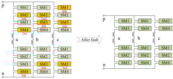
Figure 9.
The sequence of SM faults and the post-fault equivalent topology.
Figure 10 shows the three-phase bridge arm voltage and neutral point shift voltage waveform. It can be seen that the voltage waveform of the fault phase bridge arm is obviously distorted during each fault operation stage. As the number of faulty SMs increases, the voltages of the upper and lower arms of each phase are always inversely symmetrical. In the neutral point shift voltage waveform diagram, in order to make the simulation results clearer, the low-frequency signal is filtered by a low-pass filter, as shown by the solid black line. When the neutral point shift base voltage is a DC waveform and is not zero, it indicates a DC side neutral point shift. When the neutral point shift base voltage is an AC waveform, it indicates an AC side neutral point shift. When t = 0.44, all the 9 SMs are faulty. At this time, the neutral point shifts upward to 375 V and the bridge arm voltage waveform is reduced to two levels. The corresponding calculated results of fault-tolerant reconstruction parameters in each stage are shown in Table 1.

Figure 10.
The three-phase bridge arm voltage and neutral point shift voltage waveform.

Table 1.
The fault-tolerant reconstruction parameters in each stage.
Figure 11 shows the waveforms of the three-phase output phase voltage, line voltage and current. It can be seen that the amplitude variation of the phase voltage corresponds to that of the bridge arm voltage. The output line voltage and current waveforms always maintain three-phase symmetry. With the increase of the number of faulty SMs, the maximum amplitude continues to decrease and agrees with the theoretical values. When t = 0.44, all the 9 sub-modules are faulty, and the line voltage amplitude decreases to 584.55 V. The simulation results are consistent with the previous analysis.
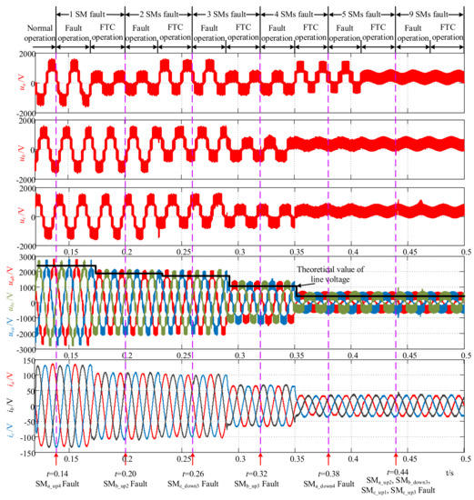
Figure 11.
The waveforms of three-phase output phase voltage, line voltage, and current.
4.2. Case 2
In this case, the faulty SMs are distributed in the upper arm of three phases. After three-phase fault information fusion, finally there is 1 sub-module remaining in the upper arm and 4 sub-modules in the lower arm. Suppose SMa_up1, SMc_up1, SMa_up2, SMa_up3, SMb_up2, SMb_up3, SMb_up4, SMc_up3 and SMc_up4 in the system have open-circuit fault in sequence and corresponding fault-tolerant control is carried out. The corresponding sequence of sub-module faults and the post-fault equivalent topology are shown in Figure 12.

Figure 12.
The sequence of sub-module faults and the post-fault equivalent topology.
Figure 13 shows the waveforms of the neutral point shift voltage, the three-phase output voltage and the output line voltage. After the fault occurs, the neutral point shift voltage varies with the increase of the number of faulty SMs. The three-phase voltage is in a symmetrical or asymmetrical state. The output line voltage is always symmetrical, and its amplitude decreases with the number of faulty SMs. When t = 0.38 s, all the 9 sub-modules are faulty. At this time, the neutral point shifts upward to 1250 V, and the output line voltage amplitude decreases to 584.55 V. The corresponding calculated results of fault-tolerant reconstruction parameters in each stage are shown in Table 2.

Figure 13.
The waveforms of the neutral point shift voltage, the three-phase output phase voltage and line voltage.
Table 2.
The fault-tolerant reconstruction parameters in each stage.
The simulation analysis in the above two cases shows that the fault-tolerant control strategy proposed in this paper can be used to calculate the fault-tolerant reconstruction shift parameters online for multiple SM faults. The output line voltage of the system after fault-tolerant control is symmetrical and the amplitude is the largest possible.
5. Experimental Verification
In this paper, the correctness of theoretical analysis and simulations is verified by constructing a low-power experimental system of three-phase MMC. The experimental system is shown in Figure 14, which mainly includes the main circuit, control circuit, power supply, and oscilloscope. Each SM in the main circuit is an Infineon’s two-unit IGBT module FF75R12RT4. The control circuit uses a joint control module consisting of DSP + FPGA, where the DSP type is TMS320F28335 and FPGA is Spartan 6 XC6SLX16 (Xilinx, San Jose, CA, USA). The oscilloscope model is Tektronix’s MDO3000 (Tektronix, Portland, OR, USA). The specific experimental parameters are as follows: DC bus voltage is , the number of SMs in each phase is 2N = 4, the inductance of the bridge arm is 3 mH, the resistance of the load resistor is 20 Ω, the load inductance is 20 mH, the carrier frequency is 2 kHz, and the base frequency of the three-phase output voltage is 50 Hz, and the modulation ratio is m = 0.8. The experimental system is shown in Figure 14.

Figure 14.
The physical map of the experimental system.
5.1. System Overall Performance Testing
Figure 15 shows the MMC output voltage waveforms in normal operation. Figure 15a is the output phase voltage waveform. The output phase voltage of each phase in one power frequency cycle is three levels, and the voltage of each level is in the order of 48 V. The overall waveform is circular, which is obviously different from the output voltage waveform of traditional converters. Figure 15b is the output line voltage waveform. The voltage is five levels in one power frequency cycle, and the phases differ by 120°. Figure 15c is the voltage waveforms of the upper and lower arms, which have the same amplitude but opposite phase, in agreement with theoretical analysis and simulation results. Figure 15d is the SM capacitor voltage waveform. It can be seen that the currently measured capacitor voltage is basically stable at 51 V, close to the theoretical value of 48 V, and the fluctuation is small, approximately 0.63%.
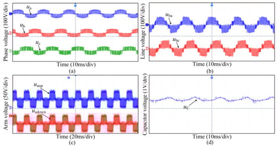
Figure 15.
The output voltage waveforms in normal operation. (a) Three-phase voltage; (b) Line voltage; (c) Arm voltage; (d) Sub-module capacitor voltage.
Figure 16a,b show the waveform of a-phase & b-phase output current and the waveform of a-phase bridge arm current after a conditioning circuit in normal operation, respectively. According to the experimental results, the output current amplitude is about 3.6 A, and the theoretical value is about A. The upper and lower arms have opposite current phases, and the amplitudes are both around 2.5 A. The experimental results are consistent with the theoretical values.

Figure 16.
The currents in normal operation. (a) Output current; (b) Arm current.
The above experimental results indicate that the experimental system can achieve the normal operation of three-phase MMC, the hardware circuit design is correct, and the software control strategy employed is in line with relevant requirements. Thus, the experimental verification is valid.
5.2. Fault-Tolerant Control Testing under Single SM Fault
Due to the limited scale of the experimental system, each bridge arm has only two SMs in normal operation. According to the previous analysis of fault tolerance capability, a single SM fault is allowed at most in each arm. Therefore, this experiment performs fault-tolerant control under a single SM fault.
Figure 17 shows the output voltage waveforms after fault-tolerant control when a single SM fault occurs in the a-phase upper arm. Figure 17a,b are the waveforms before and after the a-phase voltage fault. It can be seen that the phase voltage waveform is three levels and the amplitude is 48.2 V in normal operation. In the fault-tolerant operation after fault, as the a-phase upper arm cannot output modulation waves continuously, the DC side neutral point shifts downward. The maximum output power of the three phase voltages is reduced to half that in normal operation, the output voltage is reduced to two levels, and the amplitude is reduced to 24.4 V. Figure 17c,d are the waveforms before and after the line voltage fault. In normal operation, it is five levels and the amplitude is around 96 V. After fault, the line voltage decreases to three levels and the amplitude decreases to around 50 V. Figure 17e,f are the waveforms of the neutral point shift voltage before and after the fault. The average value is 0 V in normal operation, and in fault-tolerant operation, it shifts upward, with an average of about 50 V. Therefore, the neutral point shift at this time occurs only on the DC side. The experimental results are basically consistent with the theoretical analysis, which indicates the validity of the proposed fault-tolerant control strategy based on neutral point compound shift.
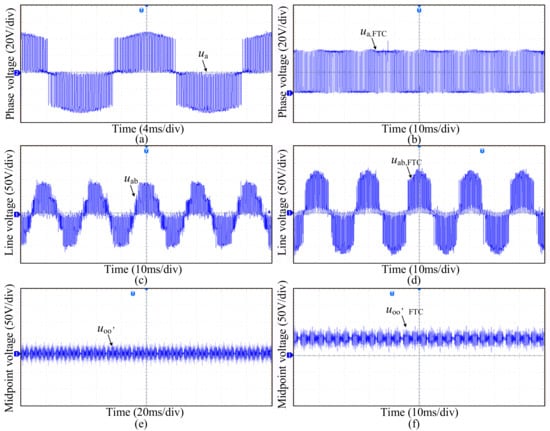
Figure 17.
The waveforms of single SM fault-tolerant control. (a) Phase voltage in normal operation; (b) Phase voltage in fault operation; (c) Line voltage in normal operation; (d) Line voltage in fault operation; (e) Neutral point shift voltage in normal operation; (f) Neutral point shift voltage in fault operation.
6. Conclusions
This paper, with modular multilevel converters as the research object, studies the fault-tolerant control optimization strategy after sub-module fault occurs. The main work and contributions can be summarized as follows:
- (1)
- The fault tolerance capability of each phase bridge arm in the MMC under PDPWM modulation is analyzed. It can be seen that the maximum number of faulty SMs allowed in each phase of the bridge arm of the system is limited, and correspondingly, the fault tolerance capability of each phase bridge arm is also limited.
- (2)
- An optimization strategy based on neutral point compound shift is proposed, and the main contributions are: (i) It realizes fast acquisition of fault-tolerant reconstruction adjustment parameters by optimizing AC side phase voltage vector reconstruction, and the calculation complexity of neutral point shift parameters is reduced considerably; (ii) Through the neutral point DC side shift control method, the number of single-arm faulty SMs that can be fault-tolerant in the MMC system could be raised from to , which makes full use of the software and hardware resources to improve the fault tolerance capability effectively; (iii) Within the fault tolerance range, the selection of an optimal neutral point can help make sure the output line voltage of the system is symmetrical and the amplitude is as large as possible after fault tolerance control.
- (3)
- The simulations in the Matlab/Simulink environment and experiments with a low-power MMC-based prototype are all studied with the proposed controller under different fault conditions. The results confirm the efficiency of the fault-tolerant control strategy proposed in this paper.
Author Contributions
Q.Z. conceived, designed the research work and modified the paper; W.D. analyzed the data; L.G. designed, performed the research work and wrote the paper; X.T., Z.L. and D.X. contributed materials/analysis tools.
Funding
This research work was supported by the National Natural Science Foundation of China, grant number 51777141.
Conflicts of Interest
The authors declare no conflict of interest.
References
- Moranchel, M.; Huerta, F.; Sanz, I.; Bueno, E.; Rodríguez, F. A Comparison of Modulation Techniques for Modular Multilevel Converters. Energies 2016, 9, 1091. [Google Scholar] [CrossRef]
- Morsy, A.; Yong, Z.; Enjeti, P. A new high power density modular multilevel DC-DC converter with localized voltage balancing control for arbitrary number of levels. In Proceedings of the IEEE Applied Power Electronics Conference & Exposition, Long Beach, CA, USA, 20–24 March 2016. [Google Scholar]
- Wen, W.; Wu, X.; Yin, J.; Long, J.; Shuai, W.; Li, J. Characteristic Analysis and Fault-Tolerant Control of Circulating Current for Modular Multilevel Converters under Sub-Module Faults. Energies 2017, 10, 1827. [Google Scholar]
- Liu, Y.; Li, D.; Yu, J.; Wang, Q.; Song, W. Research on Unbalance Fault-Tolerant Control Strategy of Modular Multilevel Photovoltaic Grid-Connected Inverter. Energies 2018, 11, 1368. [Google Scholar] [CrossRef]
- Yang, L.; Liu, J.; Wang, C. Fault diagnosis and fault tolerance control of multilevel sub-module based on HONBM self-inclusion. Comput. Electr. Eng. 2018, 72, 92–99. [Google Scholar] [CrossRef]
- Chen, J.; Sun, C.; Yang, L.; Xin, Y.; Li, B.; Li, G. The analysis of DC fault mode effects on MMC-HVDC system. In Proceedings of the Power & Energy Society General Meeting, Chicago, IL, USA, 16–20 July 2017. [Google Scholar]
- Nguyen, T.H.; Lee, D.C. A novel submodule topology of MMC for blocking DC-fault currents in HVDC transmission systems. In Proceedings of the International Conference on Power Electronics & Ecce Asia, Seoul, Korea, 1–5 June 2015. [Google Scholar]
- Li, B.; Shi, S.; Bo, W.; Wang, G.; Wei, W.; Xu, D. Fault Diagnosis and Tolerant Control of Single IGBT Open-Circuit Failure in Modular Multilevel Converters. IEEE Trans. Power Electron. 2015, 31, 3165–3176. [Google Scholar] [CrossRef]
- Son, G.T.; Lee, H.J.; Nam, T.S.; Chung, Y.H.; Lee, U.H.; Baek, S.T.; Hur, K.; Park, J.W. Design and Control of a Modular Multilevel HVDC Converter with Redundant Power Modules for Noninterruptible Energy Transfer. IEEE Trans. Power Deliv. 2012, 27, 1611–1619. [Google Scholar]
- Kai, L.; Yuan, L.; Zhao, Z.; Lu, S.; Zhang, Y. Fault-Tolerant Control of MMC with Hot Reserved Submodules Based on Carrier Phase Shift Modulation. IEEE Trans. Power Electron. 2017, 32, 6778–6791. [Google Scholar]
- Deng, F.; Tian, Y.; Zhu, R.; Zhe, C. Fault-Tolerant Approach for Modular Multilevel Converters Under Submodule Faults. IEEE Trans. Ind. Electron. 2016, 63, 7253–7263. [Google Scholar] [CrossRef]
- Song, P.; Lin, J.; Li, Y.; Wu, J. Direct power control strategy of railway static power conditioner based on modular multilevel converter. Power Syst. Technol. 2015, 9, 2511–2518. [Google Scholar]
- Li, B.; Xu, Z.; Jian, D.; Xu, D. Fault-Tolerant Control of Medium-Voltage Modular Multilevel Converters with Minimum Performance Degradation under Submodule Failures. IEEE Access 2018, 6, 11772–11781. [Google Scholar] [CrossRef]
- Lu, Z.L.Z.; Chen, Z.C.Z.; Gong, Y.G.Y.; Cao, J.C.J.; Wang, H.W.H. Sub-module fault analysis and fault-tolerant control strategy for modular multilevel converter. In Proceedings of the Iet International Conference on Ac & Dc Power Transmission, Beijing, China, 28–29 May 2016. [Google Scholar]
- Hu, P.; Jiang, D.; Zhou, Y.; Liang, Y.; Jie, G.; Lin, Z. Energy-balancing Control Strategy for Modular Multilevel Converters Under Submodule Fault Conditions. IEEE Trans. Power Electron. 2014, 29, 5021–5030. [Google Scholar] [CrossRef]
- Li, J.; Wu, X.; Yao, X.; Long, J.; Jin, X.; Wen, W.; Wang, X.; Shuai, W. A zero-sequence voltage injection control scheme for modular multilevel converter under submodule failure. Energy Convers. Congr. Expo. 2015, 121, 270–278. [Google Scholar]
- Carnielutti, F.; Pinheiro, H.; Rech, C. Generalized Carrier-Based Modulation Strategy for Cascaded Multilevel Converters Operating Under Fault Conditions. IEEE Trans. Ind. Electron. 2011, 59, 679–689. [Google Scholar] [CrossRef]
- Wu, W.; Wu, X.; Jin, L.; Li, J.; Wang, S.; Wang, X. Fault-tolerant Control Strategy of Neutral Point Shift for Sub-module Faults of Modular Multilevel Converters. Autom. Electr. Power Syst. 2016, 40, 20–26. [Google Scholar]
- Zhou, F.; An, L.; Yan, L.; Xu, Q.; Guerrero, J.M. Double-Carrier Phase-Disposition Pulse Width Modulation Method for Modular Multilevel Converters. Energies 2017, 10, 581. [Google Scholar] [CrossRef]
- Liu, L.; Yin, J.; Jin, G.; Zhou, P. Simulation of Traction Drive Control System of High-speed EMUs. Electr. Drive Autom. 2017, 39, 12–15. [Google Scholar]
© 2019 by the authors. Licensee MDPI, Basel, Switzerland. This article is an open access article distributed under the terms and conditions of the Creative Commons Attribution (CC BY) license (http://creativecommons.org/licenses/by/4.0/).