Accurate and Fast Generation of Irregular Short Crested Waves by Using Periodic Boundaries in a Mild-Slope Wave Model

Abstract

In this work, periodic lateral boundaries are developed in a time dependent mild-slope equation model, MILDwave, for the accurate generation of regular waves and irregular long and short crested waves in any direction. A single wave generation line inside the computational domain is combined with periodic lateral boundaries. This generation layout yields a homogeneous and thus accurate wave field in the whole domain in contrast to an L-shaped and an arc-shaped wave generation layout where wave diffraction patterns appear inside the computational domain as a result of the intersection of the two wave generation lines and the interaction with the lateral sponge layers. In addition, the performance of the periodic boundaries was evaluated for two different wave synthesis methods for short crested waves generation, a method proposed by Miles and a method proposed by Sand and Mynett. The results show that the MILDwave model with the addition of periodic boundaries and the Sand and Mynett method is capable of reproducing a homogeneous wave field as well as the target frequency spectrum and the target directional spectrum with a low computational cost. The overall performance of the developed model is validated with experimental results for the case of wave transformation over an elliptic shoal (Vincent and Briggs shoal experiment). The numerical results show very good agreement with the experimental data. The proposed generation layout using periodic lateral boundaries makes the mild-slope wave model, MILDwave, an essential tool to study coastal areas and wave energy converter (WEC) farms under realistic 3D wave conditions, due to its significantly small computational cost and its high numerical stability and robustness.

1. Introduction

Numerical wave propagation models are commonly used as engineering tools for the study of wave transformation in coastal areas. Berkhoff [1] derived the first elliptic mild-slope wave equation and based on this, the parabolic model [2] and the hyperbolic model [3] have been developed to predict the transformation processes of regular waves, such as wave refraction, diffraction, shoaling, and reflection. In the parabolic model, wave reflection and diffraction in the direction of wave propagation are neglected and hence it suffers from low accuracy in cases where these phenomena are significant. On the other hand, the hyperbolic model, which takes into consideration wave reflection and diffraction in the direction of wave propagation, provides higher accuracy, but more computational time compared to the parabolic model. Moreover, to study the transformation of random waves, time dependent mild-slope equations have been developed. Radder and Dingemans [4] suggested a set of canonical equations, which are based on the time dependent mild slope equations and are derived using the Hamiltonian theory of surface waves. Booij [5] proved that these equations are valid for sea bottom slopes up to 1/3. However, Suh et al. [6] extended the latter equations by including higher order bottom effect terms proportional to the square of the bottom slope and to the bottom curvature to study wave propagation on rapidly varying topography.

For numerical prediction of the wave field in a coastal area, waves are generated along the offshore boundary of the computational domain and propagate towards the coastline. However, to be able to apply a sponge layer to absorb waves reflected towards the wave generation boundary, waves should be generated inside the numerical domain and not along the boundary. This internal wave generation technique in combination with numerical wave absorbing sponge layers was firstly proposed by [7] for Peregrine’s [8] classical Boussinesq equations. Later, Lee and Suh [9] achieved wave generation for the mild slope equations of [3] and [4] by applying the source term addition method. The main observation was that the energy of the incident waves can be properly obtained from the viewpoint of energy transport. To generate multidirectional waves, they applied an L-shaped wave generator, which is generally composed of two wave generation lines; one parallel to the x-axis and one parallel to the y-axis of the numerical domain as well as wave absorbing sponge layers behind the two wave generation lines. However, wave diffraction patterns appear inside the computational domain as a result of the intersection of the two wave generation lines and due to the interaction with the lateral sponge layers. To deal with this problem, Lee and Yoon [10] proposed an arc-shaped wave generation line; two parallel lines connected to a semicircle to avoid wave diffraction caused at the intersection of the previous wave generation lines. Further, Kim and Lee [11] used an arc-shaped source band that gives smaller errors than the Lee and Yoon [10] method, especially for a coarse grid size. Recently, Lin and Yu [12] proposed a promising method for non-reflective boundaries in a mild-slope wave model to avoid the use of sponge layers. However, in non-reflective boundaries, the level of re-reflection strongly depends on the initial approximations since the characteristics of the reflected waves (i.e., wave angle, wave celerity) inside the numerical domain cannot be estimated a priori.

In the present paper, a wave generation layout using periodic lateral boundaries is developed where a single internal wave generation line parallel to the y-axis is combined with periodic lateral boundaries at the top and bottom of the domain. With this technique, the information leaving one end of the numerical domain enters the opposite end and thus no lateral sponges are required. In this way, the wave diffraction patterns that appear inside the computational domain as a result of the intersection of the two wave generation lines and due to the interaction with the lateral sponge layers (see Figure 1) are avoided. In Figure 1, the water surface elevation, η, is presented for a regular wave field generated by an L-shaped wave generator (red dashed lines) at an angle, θ = 45°, from the x-axis. The absence of uniformity of the surface elevation along the crests and troughs, which can be observed in the same figure, is a sign of the existence of diffraction patterns inside the numerical domain.

Periodic boundaries are implemented in a time dependent mild-slope equation model, MILDwave, developed at Ghent University [13] in order to accurately generate regular and irregular waves in any direction. In addition, the performance of the periodic boundaries is evaluated for two different wave synthesis methods to generate short crested waves, a method proposed by Miles [14] and a method proposed by Sand and Mynett [15]. The mild-slope equations of Radder and Dingemans [4] without the extension of Suh et al. [6] are the basic equations employed in the phase-resolving model, MILDwave, used to simulate wave transformation processes, such as refraction, shoaling, reflection, transmission, and diffraction, intrinsically [16]. MILDwave has previously been used to predict wave diffraction and wave penetration inside harbours [17] and to study wave power conversion applications [18,19,20]. One of the challenges in the field of renewable energies is to determine the optimal geometrical layout for wave energy converter (WEC) farms, targeting the maximum possible energy production and the correct assessment of the impact of WEC farms on the wave field. To do so, accurate and detailed numerical modelling of WEC farms under realistic 3D wave conditions is considered crucial. This kind of application requires a homogeneous wave field in the whole numerical domain. To the present authors’ knowledge, periodic boundaries, which are commonly used in non-hydrostatic models [21] and Boussinesq models [22], have not been used before in a mild-slope wave model to study short crested waves. So, the novelty of the present work concerns the capability of accurate and fast generation of such homogeneous wave fields with periodic boundaries in MILDwave. In engineering applications, where non-linearities are not significant, mild-slope wave models are preferred instead of Boussinesq models or non-hydrostatic models due to their significantly smaller computational cost and their high numerical stability and robustness, and thus further development of these models should be encouraged. The implementation of periodic boundaries is important as it introduces noteworthy improvements in mild-slope models, which can then make full use of their benefits for the study of WEC farms under oblique long crested regular and irregular waves or short crested waves (real sea waves).

In the next section, a short description of the mild-slope wave propagation model, MILDwave, and the methodology of the implemented periodic boundaries are presented. Section 3 provides a detailed overview of the model results for regular and irregular long and short crested waves. In Section 4, the validation results are presented where the accuracy of the developed model is compared with experimental data. The last section provides conclusions and a summary discussion of the present study.

2. Numerical Methodology

2.1. The Mild-Slope Wave Propagation Model, MILDwave

MILDwave is a mild-slope wave propagation model based on the depth integrated time dependent mild-slope equations of Radder and Dingemans [4]. These are given in Equations (1) and (2) and describe the transformation of linear irregular waves with a narrow frequency band over a mildly varying bathymetry (bottom slopes up to 1/3):

$$\frac{\partial \mathsf{\eta }}{\partial \mathrm{t}}=\mathrm{B}\mathsf{\phi }-\nabla ·\left(\mathrm{A}\nabla \mathsf{\phi }\right)$$

(1)

$$\frac{\partial \mathsf{\phi }}{\partial \mathrm{t}}=-\mathrm{g}\mathsf{\eta }$$

(2)

where $\mathsf{\eta }\left(\mathrm{x},\mathrm{y},\mathrm{t}\right)$ and $\mathsf{\varphi }\left(\mathrm{x},\mathrm{y},\mathrm{t}\right)$ are, respectively, the surface elevation and the velocity potential at the still water level, ∇ is the horizontal gradient operator, $\mathrm{t}$ is the time, and $\mathrm{g}$ is the gravitational acceleration. The coefficients, A and B, are calculated using Equations (3) and (4), respectively:

$$\mathrm{A}=\frac{{\mathrm{CC}}_{\mathrm{g}}}{\mathrm{g}}$$

(3)

$$\mathrm{B}=\frac{{\mathsf{\omega }}^2-{\mathrm{k}}^2{\mathrm{CC}}_{\mathrm{g}}}{\mathrm{g}}$$

(4)

with $\mathrm{C}$ the phase velocity and ${\mathrm{C}}_{\mathrm{g}}$ is the group velocity for a wave with a wave number, $\mathrm{k}$, angular frequency, $\mathsf{\omega }$, wavelength, ${\mathrm{L}}_w$, and frequency, $\mathrm{f}$. For irregular waves, $\mathrm{C}$, ${\mathrm{C}}_{\mathrm{g}}$, $\mathrm{k}$, and $\mathsf{\omega }$ are replaced by the wave characteristics for the carrier frequency, $\overline{\mathrm{f}}$.

A finite difference scheme, as described in [23], is used to discretize and solve Equations (1) and (2). The domain is divided in grid cells with dimensions, $\mathsf{\Delta }\mathrm{x}$ and $\mathsf{\Delta }\mathrm{y}$, and central differences are used both for spatial and time derivatives. Both $\mathsf{\eta }$ and $\mathsf{\varphi }$ are calculated at the center of each grid cell at different time levels, $\left(\mathrm{n}+1/2\right)\mathsf{\Delta }\mathrm{t}$ and $\left(\mathrm{n}+1\right)\mathsf{\Delta }\mathrm{t}$ as:

$$\begin{array}{ll}{\mathsf{\eta }}_{\mathrm{i},\mathrm{j}}^{\mathrm{n}+1/2}\simeq {\mathsf{\eta }}_{\mathrm{i},\mathrm{j}}^{\mathrm{n}-1/2}& +{\mathrm{B}}_{\mathrm{i},\mathrm{j}}{\mathsf{\varphi }}_{\mathrm{i},\mathrm{j}}^{\mathrm{n}}\mathsf{\Delta }\mathrm{t}-\frac{{\mathrm{A}}_{\mathrm{i}+1,\mathrm{j}}-{\mathrm{A}}_{\mathrm{i}-1,\mathrm{j}}}{2\mathsf{\Delta }\mathrm{x}}\frac{{\mathsf{\varphi }}_{\mathrm{i}+1,\mathrm{j}}^{\mathrm{n}}-{\mathsf{\varphi }}_{\mathrm{i}-1,\mathrm{j}}^{\mathrm{n}}}{2\mathsf{\Delta }\mathrm{x}}\mathsf{\Delta }\mathrm{t}\\ & -{\mathrm{A}}_{\mathrm{i},\mathrm{j}}\frac{{\mathsf{\varphi }}_{\mathrm{i}-1,\mathrm{j}}^{\mathrm{n}}-2{\mathsf{\varphi }}_{\mathrm{i},\mathrm{j}}^{\mathrm{n}}+{\mathsf{\varphi }}_{\mathrm{i}+1,\mathrm{j}}^{\mathrm{n}}}{{\mathsf{\Delta }\mathrm{x}}^2}\mathsf{\Delta }\mathrm{t}\\ & -\frac{{\mathrm{A}}_{\mathrm{i},\mathrm{j}+1}-{\mathrm{A}}_{\mathrm{i},\mathrm{j}-1}}{2\mathsf{\Delta }\mathrm{y}}\frac{{\mathsf{\varphi }}_{\mathrm{i},\mathrm{j}+1}^{\mathrm{n}}-{\mathsf{\varphi }}_{\mathrm{i},\mathrm{j}-1}^{\mathrm{n}}}{2\mathsf{\Delta }\mathrm{y}}\mathsf{\Delta }\mathrm{t}\\ & -{\mathrm{A}}_{\mathrm{i},\mathrm{j}}\frac{{\mathsf{\varphi }}_{\mathrm{i},\mathrm{j}-1}^{\mathrm{n}}-2{\mathsf{\varphi }}_{\mathrm{i},\mathrm{j}}^{\mathrm{n}}+{\mathsf{\varphi }}_{\mathrm{i},\mathrm{j}+1}^{\mathrm{n}}}{{\mathsf{\Delta }\mathrm{y}}^2}\mathsf{\Delta }\mathrm{t}\end{array}$$

(5)

$${\mathsf{\varphi }}_{\mathrm{i},\mathrm{j}}^{\mathrm{n}+1}\simeq {\mathsf{\varphi }}_{\mathrm{i},\mathrm{j}}^{\mathrm{n}}-{\mathrm{g}\mathsf{\eta }}_{\mathrm{i},\mathrm{j}}^{\mathrm{n}+1/2}\mathsf{\Delta }\mathrm{t}$$

(6)

where $\mathrm{A}$ and $\mathrm{B}$ are given by Equations (3) and (4) and the superscripts and subscripts stand for the relevant time step and the relevant cell of the grid, respectively.

In the current configuration of MILDwave, the boundary conditions are formed in such a way that one layer of ghost cells is considered at each boundary. The values at the cells closest to the boundary are copied to the ghost cells and thus the layer of the ghost cells acts as a fully reflective boundary (solid wall). However, the effect of the fully reflective domain boundaries is negligible because absorbing sponge layers are applied at the outside boundaries to dissipate the incoming wave energy.

The grid cell size, $\mathsf{\Delta }\mathrm{x}=\mathsf{\Delta }\mathrm{y}$, is chosen so that ${\mathrm{L}}_{\mathrm{w}}/20\le \mathsf{\Delta }\mathrm{x}=\mathsf{\Delta }\mathrm{y}\le {\mathrm{L}}_{\mathrm{w}}/10$ (for irregular waves, ${\mathrm{L}}_{\mathrm{w}}$ = shortest wave length (maximum wave frequency)) while the time step meets the Courant-Friedrichs-Lewy criterion to guarantee a stable and consistent result.

In MILDwave, waves are generated along a wave generation line near the offshore boundary by applying the source term addition method proposed by [9] where the source term propagates with the energy velocity. According to this method, additional surface elevation, ${\mathsf{\eta }}^{\ast }$, is added with the desired energy to the calculated surface elevation, $\mathsf{\eta }$, at the wave generation line for each time step and is given by:

$${\mathsf{\eta }}^{\ast }=2{\mathsf{\eta }}^{\mathrm{I}}\frac{{\mathrm{C}}_{\mathrm{e}}\mathsf{\Delta }\mathrm{t}}{\mathsf{\Delta }\mathrm{x}}\cos \mathsf{\theta }$$

(7)

where $\mathsf{\Delta }\mathrm{x}$ is the grid size in the x-axis, $\mathsf{\Delta }\mathrm{t}$ is the time step, $\mathsf{\theta }$ is the wave propagation angle with respect to the x-axis, ${\mathsf{\eta }}^{\mathrm{I}}$ the water surface elevation of incident waves, and ${\mathrm{C}}_{\mathrm{e}}$ is the energy velocity given by Equation (8):

$${\mathrm{C}}_{\mathrm{e}}=\overline{{\mathrm{C}}_{\mathrm{g}}}\frac{\overline{\mathsf{\omega }}}{\mathsf{\omega }}\sqrt{1+\frac{\overline{\mathrm{C}}}{\overline{{\mathrm{C}}_{\mathrm{g}}}}\left({\left(\frac{\mathsf{\omega }}{\overline{\mathsf{\omega }}}\right)}^2-1\right)}$$

(8)

where the bar indicates that the variable is associated with the carrier angular frequency, $\overline{\mathsf{\omega }}$.

It has been proven that the model of [4] can be used to simulate the transformation of long and short crested waves. To generate long crested irregular waves, a parameterized JONSWAP (Joint North Sea Wave Observation Project) spectrum, $\mathrm{S}\left(\mathrm{f}\right)$ (Equation (9)), or a TMA (Texel, Marsen, Arsloe) spectrum (Equation (10)), which can be applied in shallow water, has been used as an input spectrum:

$$\mathrm{S}\left(\mathrm{f}\right)=\frac{0.0624}{0.230+0.0336\mathsf{\gamma }-\frac{0.185}{1.9+\mathsf{\gamma }}}{\mathrm{H}}_{\mathrm{s}}{}^2{\mathrm{f}}_{\mathrm{p}}{}^4{\mathrm{f}}^{-5}{\mathsf{\gamma }}^{\exp \left(-\frac{{\left(\mathrm{f}-{\mathrm{f}}_{\mathrm{p}}\right)}^2}{2{\mathsf{\sigma }}^2{\mathrm{f}}_{\mathrm{p}}{}^2}\right)}\exp \left(-\frac{5}{4}{\left(\frac{{\mathrm{f}}_{\mathrm{p}}}{\mathrm{f}}\right)}^4\right)$$

(9)

$$\mathrm{S}\left(\mathrm{f}\right)=\frac{{\mathsf{\alpha }\mathrm{g}}^2}{{\left(2\mathsf{\pi }\right)}^4{\mathrm{f}}^5}\exp \left(-\frac{5}{4}{\left(\frac{{\mathrm{f}}_{\mathrm{p}}}{\mathrm{f}}\right)}^4+\left(\ln \mathsf{\gamma }\right)\exp \left(-\frac{{\left(\mathrm{f}-{\mathrm{f}}_{\mathrm{p}}\right)}^2}{2{\mathsf{\sigma }}^2{\mathrm{f}}_{\mathrm{p}}{}^2}\right)\right)\mathsf{\varphi }\left(\mathrm{f},\mathrm{d}\right)$$

(10)

where ${\mathrm{H}}_{\mathrm{s}}$ is the significant wave height, ${\mathrm{f}}_{\mathrm{p}}$ is the peak wave frequency, $\mathsf{\gamma }$ is the peak enhancement factor, $\mathsf{\alpha }$ is the Phillips constant, and $\mathsf{\sigma }$ is the spectral width parameter, which depends on the value of the wave frequency:

$$\mathsf{\sigma }=\{\begin{array}{c}0.07 f\le {\mathrm{f}}_{\mathrm{p}}\\ 0.09 f\ge {\mathrm{f}}_{\mathrm{p}}\end{array}$$

(11)

The frequency dependent factor, $\mathsf{\varphi }\left(\mathrm{f},\mathrm{d}\right),$ which takes into account the effect of a finite water depth, $\mathrm{d}$, is given by:

$$\mathsf{\varphi }\left(\mathrm{f},\mathrm{d}\right)=\{\begin{array}{c}0.5{\mathsf{\omega }}_{\mathrm{h}}{}^2,\\ 1-0.5{\left(2-{\mathsf{\omega }}_{\mathrm{h}}\right)}^2,\\ 1,\end{array}\begin{array}{l}{\mathsf{\omega }}_{\mathrm{h}}<1\\ 1\le {\mathsf{\omega }}_{\mathrm{h}}\le 2\\ {\mathsf{\omega }}_{\mathrm{h}}>2\end{array},{\mathsf{\omega }}_{\mathrm{h}}=2\mathsf{\pi }\mathrm{f}\sqrt{\frac{\mathrm{d}}{\mathrm{g}}}$$

(12)

To generate short crested waves, two different wave synthesis methods are employed in the present study, a single summation method proposed by [14] and a second single summation method proposed by [15]. In single summation models, each wave component must have a unique frequency and each frequency component can only travel in one direction, while several wave components are travelling in the same direction. According to the Miles method, the surface elevation is defined as follows:

$$\mathsf{\eta }\left(\mathrm{x},\mathrm{y},\mathrm{t}\right)={\displaystyle \sum }_{\mathrm{n}=1}^{\mathrm{N}}{\displaystyle \sum }_{\mathrm{m}=1}^{\mathrm{M}}{\mathrm{A}}_{\mathrm{nm}}\cos ({\mathsf{\omega }}_{\mathrm{nm}}\mathrm{t}-{\mathrm{k}}_{\mathrm{nm}}\left(\mathrm{x}\cos {\mathsf{\theta }}_{\mathrm{m}}+\mathrm{y}\sin {\mathsf{\theta }}_{\mathrm{m}}\right)+{\mathsf{\epsilon }}_{\mathrm{nm}})$$

(13)

with the wave amplitude, ${\mathrm{A}}_{\mathrm{nm}}=\sqrt{2\mathrm{S}\left({\mathrm{f}}_{\mathrm{nm}}\right)\mathrm{D}\left({\mathrm{f}}_{\mathrm{nm}},{\mathsf{\theta }}_{\mathrm{m}}\right)\mathrm{M}\mathsf{\Delta }\mathrm{f}\mathsf{\Delta }\mathsf{\theta }}$, the wave angular frequency, ${\mathsf{\omega }}_{\mathrm{nm}}=2{\mathsf{\pi }\mathrm{f}}_{\mathrm{nm}}=2\mathsf{\pi }\left(\mathrm{M}\left(\mathrm{n}-1\right)+\mathrm{m}\right)\mathsf{\Delta }\mathrm{f}+2{\mathsf{\pi }\mathrm{f}}_{\min }$, the frequency interval, $\mathsf{\Delta }\mathrm{f}=\frac{{\mathrm{f}}_{\max }-{\mathrm{f}}_{\min }}{\mathrm{NM}-1}$, the wave propagation angle, ${\mathsf{\theta }}_{\mathrm{m}}=\left(\mathrm{m}-1\right)\mathsf{\Delta }\mathsf{\theta }+{\mathsf{\theta }}_0-{\mathsf{\theta }}_{\max }$, the wave propagation angle interval, $\mathsf{\Delta }\mathsf{\theta }=\frac{2{\mathsf{\theta }}_{\max }}{\mathrm{M}-1}$, the random phase, ${\mathsf{\epsilon }}_{\mathrm{nm}}$, and the maximum discrete wave direction, ${\mathsf{\theta }}_{\max }$. In this way, the directional spreading function is discretized into M equally spaced wave directions ranging from ${\mathsf{\theta }}_{\min }$ to ${\mathsf{\theta }}_{\max }$.

Sand and Mynett [15] proposed a method in which the directional spectrum is decomposed as follows:

$$\mathsf{\eta }\left(\mathrm{x},\mathrm{y},\mathrm{t}\right)={\displaystyle \sum }_{\mathrm{n}=1}^{\mathrm{N}}\sqrt{2\mathrm{S}\left({\mathrm{f}}_{\mathrm{n}}\right)\mathsf{\Delta }\mathrm{f}}\cos ({\mathsf{\omega }}_{\mathrm{n}}\mathrm{t}-{\mathrm{k}}_{\mathrm{n}}\left(\mathrm{x}\cos {\mathsf{\theta }}_{\mathrm{n}}+\mathrm{y}\sin {\mathsf{\theta }}_{\mathrm{n}}\right)+{\mathsf{\epsilon }}_{\mathrm{n}})$$

(14)

In this method, the wave propagation angles are selected at random according to the cumulative distribution function of the directional spreading function, $\mathrm{D}\left(\mathrm{f},\mathsf{\theta }\right)$, and are assigned to each frequency component. The Miles method [14] provides an accurate representation of the targeted spreading function shape, but introduces different localized distortions in the frequency spectrum to obtain a close fit to the spreading function. On the other hand, the Sand and Mynett method [15] yields an exact match to the frequency spectrum.

Several semi-empirical proposed formulations of the directional spreading function, $\mathrm{D}\left(\mathrm{f},\mathsf{\theta }\right)$, have been reported, most of which consider the spreading function to be independent of the wave frequency. Here, an alternative of the well-known spreading function of [24] is employed [25]:

$$\begin{array}{cc}\mathrm{D}\left(\mathrm{f},\mathsf{\theta }\right)=\frac{1}{\sqrt{\mathsf{\pi }}}\frac{\mathsf{\Gamma }\left({\mathrm{s}}_1+1\right)}{\mathsf{\Gamma }\left({\mathrm{s}}_1+\frac{1}{2}\right)}{\cos }^{2{\mathrm{s}}_1}\left(\mathsf{\theta }-{\mathsf{\theta }}_0\right),& -\frac{\mathsf{\pi }}{2}<\mathsf{\theta }-{\mathsf{\theta }}_0<\end{array}\frac{\mathsf{\pi }}{2}$$

(15)

where ${\mathrm{s}}_1$ is the directional spreading parameter, $\mathsf{\Gamma }$ is the Gamma function, and ${\mathsf{\theta }}_0$ is the wave propagation angle.

To derive the relation between the directional spreading parameter, ${\mathrm{s}}_1$, and the spreading standard deviation, ${\mathsf{\sigma }}_{\mathsf{\theta }}$, which is called the directional width, the methodology of [26] is followed:

$${\mathsf{\sigma }}_{\mathsf{\theta }}=\sqrt{2\left(1-\sqrt{{\left({{\displaystyle \int }}_0^{2\mathsf{\pi }}\mathrm{D}\left(\mathrm{f},\mathsf{\theta }\right)\sin \mathsf{\theta }\mathrm{d}\mathsf{\theta }\right)}^2+{\left({{\displaystyle \int }}_0^{2\mathsf{\pi }}\mathrm{D}\left(\mathrm{f},\mathsf{\theta }\right)\cos \mathrm{d}\mathsf{\theta }\right)}^2}\right)}$$

(16)

Substitution of Equation (15) into Equation (16) yields:

$${\mathsf{\sigma }}_{\mathsf{\theta }}=\sqrt{2-\frac{2{\mathsf{\Gamma }}^2\left({\mathrm{s}}_1+1\right)}{\mathsf{\Gamma }\left({\mathrm{s}}_1+\frac{1}{2}\right)\mathsf{\Gamma }\left({\mathrm{s}}_1+\frac{3}{2}\right)}}$$

(17)

The relation between ${\mathrm{s}}_1$ and ${\mathsf{\sigma }}_{\mathsf{\theta }}$ is indicated in Figure 2. Hence, fixed values of ${\mathrm{s}}_1$ and ${\mathsf{\sigma }}_{\mathsf{\theta }}$ can be determined for wind and swell waves:

$${\mathrm{s}}_1=\{\begin{array}{c}1.17 \\ 15.8 \end{array}\begin{array}{c}\to {\mathsf{\sigma }}_{\mathsf{\theta }}=30°\\ \to {\mathsf{\sigma }}_{\mathsf{\theta }}=10°\end{array}\begin{array}{c}\left(\mathrm{wind}\mathrm{waves}\right)\\ \left(\mathrm{swell}\mathrm{waves}\right)\end{array}$$

(18)

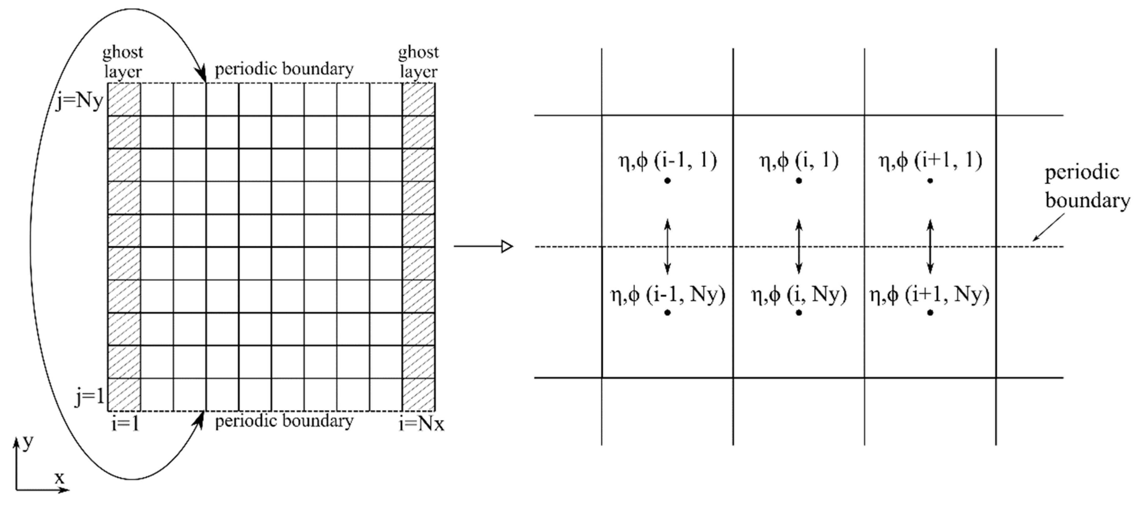
2.2. Periodic Boundaries

To create a homogeneous wave field of oblique long crested regular and irregular waves or short crested waves, periodic lateral boundaries have been implemented. In the present study, a single wave generation line parallel to the y-axis is combined with periodic lateral boundaries at the top and bottom of the domain. In this way, the information leaving one end of the numerical domain enters the opposite end and thus the required model length in this direction is reduced. This technique can lead to a more homogeneous wave field than an L-shaped and an arc-shaped wave generation since no wave diffraction problems are caused by the presence of lateral sponge layers and the intersection of the two wave generation lines (Figure 1).

Figure 3 is a schematic representation of the way that the periodic boundaries are working. Firstly, the left part of the figure presents the numerical domain under investigation, with the squares representing a random number of cells where $\mathrm{Nx}$ and $\mathrm{Ny}$ is the number of cells in the x and y direction, respectively. A layer of ghost cells is present next to each vertical boundary, acting as a fully reflective wall as described in the previous section. On the other hand, the dashed lines, which are parallel to the x-axis, represent the periodic boundaries.

At the position of the periodic boundaries, Equation (5) is solved considering that the two boundaries are adjacent, as it can be observed from the right part of Figure 3, yielding Equations (19) and (20) instead of Equation (5) for the bottom ($\mathrm{j}$ = 1) and top ($\mathrm{j}$ = $\mathrm{Ny}$) layer of cells, respectively:

$$\begin{array}{l}{\mathsf{\eta }}_{\mathrm{i},1}^{\mathrm{n}+1/2}\simeq {\mathsf{\eta }}_{\mathrm{i},1}^{\mathrm{n}-1/2}+{\mathrm{B}}_{\mathrm{i},1}{\mathsf{\varphi }}_{\mathrm{i},1}^{\mathrm{n}}\mathsf{\Delta }\mathrm{t}\\ -\frac{{\mathrm{A}}_{\mathrm{i}+1,1}-{\mathrm{A}}_{\mathrm{i}-1,1}}{2\mathsf{\Delta }\mathrm{x}}\frac{{\mathsf{\varphi }}_{\mathrm{i}+1,1}^{\mathrm{n}}-{\mathsf{\varphi }}_{\mathrm{i}-1,1}^{\mathrm{n}}}{2\mathsf{\Delta }\mathrm{x}}\mathsf{\Delta }\mathrm{t}\\ -{\mathrm{A}}_{\mathrm{i},1}\frac{{\mathsf{\varphi }}_{\mathrm{i}-1,1}^{\mathrm{n}}-2{\mathsf{\varphi }}_{\mathrm{i},1}^{\mathrm{n}}+{\mathsf{\varphi }}_{\mathrm{i}+1,1}^{\mathrm{n}}}{{\mathsf{\Delta }\mathrm{x}}^2}\mathsf{\Delta }\mathrm{t}\\ -\frac{{\mathrm{A}}_{\mathrm{i},2}-{\mathrm{A}}_{\mathrm{i},\mathrm{Ny}}}{2\mathsf{\Delta }\mathrm{y}}\frac{{\mathsf{\varphi }}_{\mathrm{i},2}^{\mathrm{n}}-{\mathsf{\varphi }}_{\mathrm{i},\mathrm{Ny}}^{\mathrm{n}}}{2\mathsf{\Delta }\mathrm{y}}\mathsf{\Delta }\mathrm{t}\\ -{\mathrm{A}}_{\mathrm{i},\mathrm{j}}\frac{{\mathsf{\varphi }}_{\mathrm{i},\mathrm{Ny}}^{\mathrm{n}}-2{\mathsf{\varphi }}_{\mathrm{i},1}^{\mathrm{n}}+{\mathsf{\varphi }}_{\mathrm{i},2}^{\mathrm{n}}}{{\mathsf{\Delta }\mathrm{y}}^2}\mathsf{\Delta }\mathrm{t}\end{array}$$

(19)

$$\begin{array}{l}{\mathsf{\eta }}_{\mathrm{i},\mathrm{Ny}}^{\mathrm{n}+1/2}\simeq {\mathsf{\eta }}_{\mathrm{i},\mathrm{Ny}}^{\mathrm{n}-1/2}+{\mathrm{B}}_{\mathrm{i},\mathrm{Ny}}{\mathsf{\varphi }}_{\mathrm{i},\mathrm{Ny}}^{\mathrm{n}}\mathsf{\Delta }\mathrm{t}\\ -\frac{{\mathrm{A}}_{\mathrm{i}+1,\mathrm{Ny}}-{\mathrm{A}}_{\mathrm{i}-1,\mathrm{Ny}}}{2\mathsf{\Delta }\mathrm{x}}\frac{{\mathsf{\varphi }}_{\mathrm{i}+1,\mathrm{Ny}}^{\mathrm{n}}-{\mathsf{\varphi }}_{\mathrm{i}-1,\mathrm{Ny}}^{\mathrm{n}}}{2\mathsf{\Delta }\mathrm{x}}\mathsf{\Delta }\mathrm{t}\\ -{\mathrm{A}}_{\mathrm{i},\mathrm{j}}\frac{{\mathsf{\varphi }}_{\mathrm{i}-1,\mathrm{Ny}}^{\mathrm{n}}-2{\mathsf{\varphi }}_{\mathrm{i},\mathrm{Ny}}^{\mathrm{n}}+{\mathsf{\varphi }}_{\mathrm{i}+1,\mathrm{Ny}}^{\mathrm{n}}}{{\mathsf{\Delta }\mathrm{x}}^2}\mathsf{\Delta }\mathrm{t}\\ -\frac{{\mathrm{A}}_{\mathrm{i},1}-{\mathrm{A}}_{\mathrm{i},\mathrm{Ny}-1}}{2\mathsf{\Delta }\mathrm{y}}\frac{{\mathsf{\varphi }}_{\mathrm{i},1}^{\mathrm{n}}-{\mathsf{\varphi }}_{\mathrm{i},\mathrm{Ny}-1}^{\mathrm{n}}}{2\mathsf{\Delta }\mathrm{y}}\mathsf{\Delta }\mathrm{t}\\ -{\mathrm{A}}_{\mathrm{i},\mathrm{j}}\frac{{\mathsf{\varphi }}_{\mathrm{i},\mathrm{Ny}-1}^{\mathrm{n}}-2{\mathsf{\varphi }}_{\mathrm{i},\mathrm{Ny}}^{\mathrm{n}}+{\mathsf{\varphi }}_{\mathrm{i},1}^{\mathrm{n}}}{{\mathsf{\Delta }\mathrm{y}}^2}\mathsf{\Delta }\mathrm{t}\end{array}$$

(20)

This implementation is valid under the assumption that the bathymetry close to the lateral boundaries is uniform for the waves to pass from one boundary to the other without any distortion and thus the continuity to be satisfied. In addition, the distance between the two boundaries should be an integer multiple of the wavelength to avoid phase differences. To ensure that this requirement is valid, the wave propagation angle, $\mathsf{\theta }$, of each wave component is slightly adjusted such that Equation (21) is satisfied [27]:

$$\mathrm{k}\sin \mathsf{\theta }=\mathsf{\alpha }\frac{2\mathsf{\pi }}{{\mathrm{L}}_{\mathrm{per}}}$$

(21)

where $\mathrm{k}$ is the wave number of each wave component, $\mathsf{\alpha }$ is an integer, and ${\mathrm{L}}_{\mathrm{per}}$ (${\mathrm{L}}_{\mathrm{per}}=\mathsf{\Delta }\mathrm{y}\ast \mathrm{Ny}$) is the periodicity length.

This means that the simulated wave propagation angle slightly deviates from the input wave angle. To minimize this deviation, the periodicity length, ${\mathrm{L}}_{\mathrm{per}}$, of the computational domain should be carefully chosen to be larger than one periodic wave length, ${\mathrm{L}}_{\mathrm{y}}$ (${\mathrm{L}}_{\mathrm{y}}={\mathrm{L}}_{\mathrm{w}}/\sin \mathsf{\theta }$) [28]. Hence, in the case of irregular long crested waves, each wave component propagates in a slightly different direction than the mean value and a directional spread of the wave energy occurs. However, it has been verified that the spreading standard deviation, ${\mathsf{\sigma }}_{\mathsf{\theta }}$, is very small (${\mathsf{\sigma }}_{\mathsf{\theta }}<$ 2°) and the waves can be considered as uni-directional.

3. Results by the Model, MILDwave

In this section, the applicability and accuracy of periodic boundaries to propagate regular and irregular long and short crested waves over a flat bottom is examined. For the evaluation of the numerical simulation results, a common method is followed. The results for a series of test cases are presented in terms of a disturbance coefficient, ${\mathrm{k}}_{\mathrm{d}}$, for the entire numerical domain. For regular waves, ${\mathrm{k}}_{\mathrm{d}}$ is given by the ratio, $\mathrm{H}/{\mathrm{H}}_{\mathrm{GB}}$, where $\mathrm{H}$ is the local wave height and ${\mathrm{H}}_{\mathrm{GB}}$ is the wave height at the wave generation boundary. In the case of irregular waves, the significant wave heights are used to calculate the ${\mathrm{k}}_{\mathrm{d}}$ value (${\mathrm{H}}_{\mathrm{s}}/{\mathrm{H}}_{\mathrm{sGB}}$). For all test cases, the numerical basin is 20 ${\mathrm{L}}_{\mathrm{w}}$ long and 20 ${\mathrm{L}}_{\mathrm{w}}$ wide (where ${\mathrm{L}}_{\mathrm{w}}$ is the wave length and is equal to ${\mathrm{L}}_{\mathrm{w}}$ = 100 m) while a uniform water depth, $\mathrm{d}$ = 7.5 m, is used. Thus, in the following numerical tests, the target wave field is a homogeneous one. A homogeneous wave field is characterized by the lack of significant fluctuations from the target, ${\mathrm{k}}_{\mathrm{d}}$, value, which is equal to ${\mathrm{k}}_{{\mathrm{d}}_{\mathrm{t}}}$ = 1.

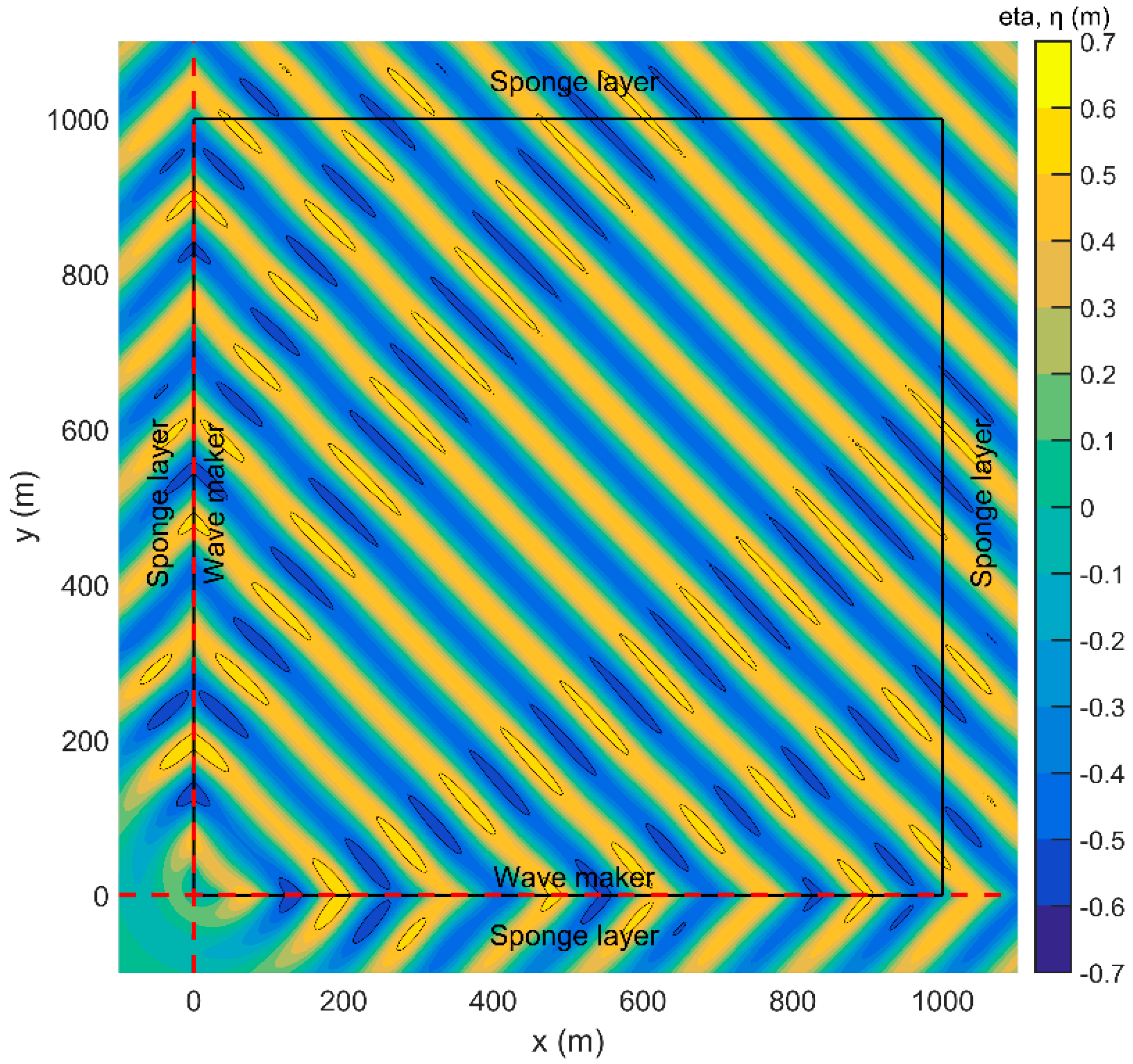
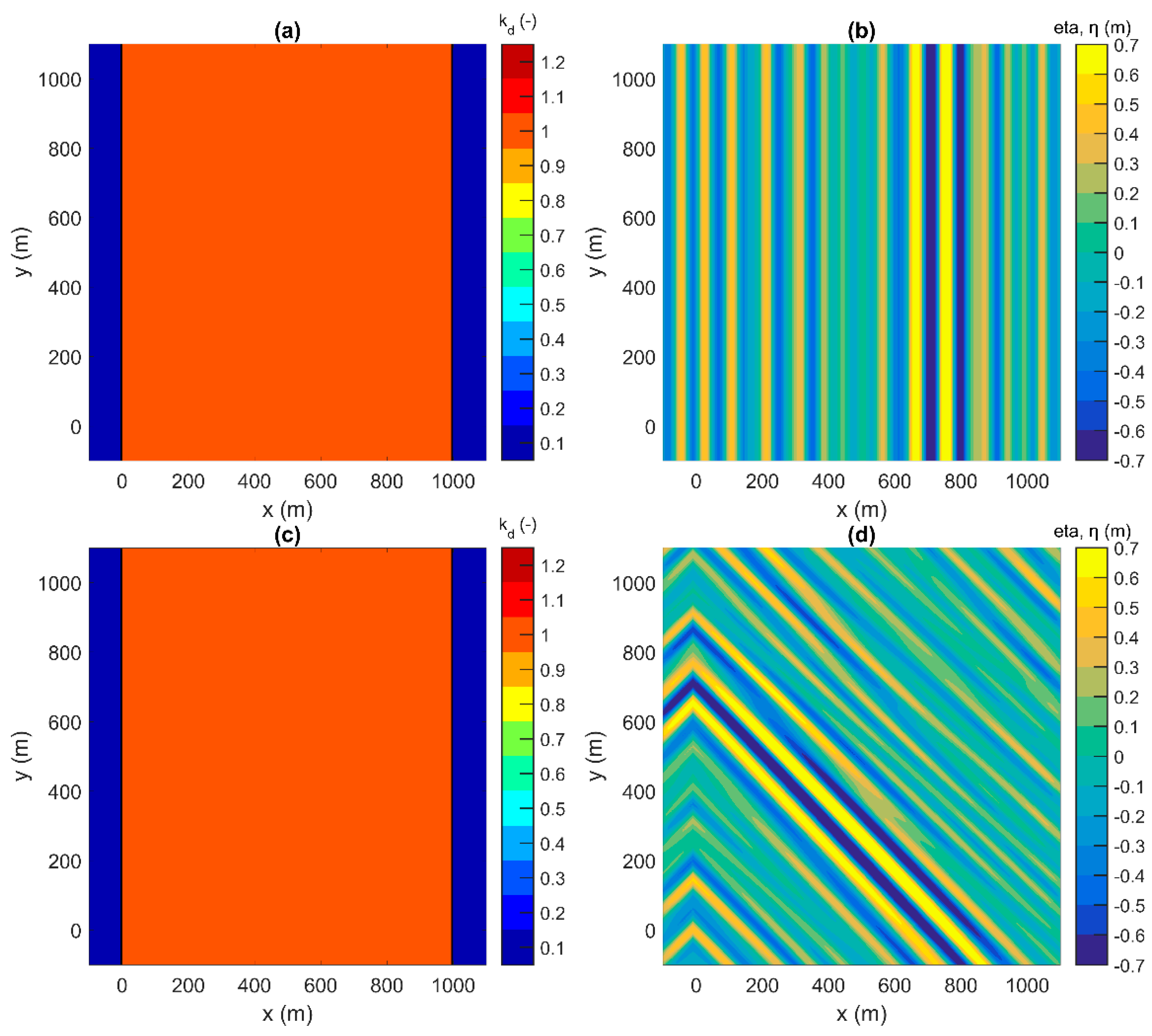
3.1. Generation of Regular Waves

Firstly, oblique regular waves are examined to compare three different wave generation layouts. The first wave generation layout (Figure 4a) is an L-shaped wave generator, which is composed by two orthogonal lines as proposed by [9]. The two wave generation lines intersect at a point outside the sponge layers and they extend to the computational domain boundary. The hatched areas indicate the areas of the numerical domain covered by wave absorbing sponge layers. These sponge layers are necessary to absorb waves reflected by the numerical domain boundaries and by structures. The second wave generation layout (Figure 4b) is based on the method suggested by [10], who proposed an arc-shaped wave generation layout where two parallel lines are connected to a semicircle. Figure 4c shows the third wave generation layout that is the main research object of the present paper, in which a single wave generation line parallel to the y-axis is combined with periodic lateral boundaries at the top and bottom of the domain. This means that the computational grid is repeated in the y-direction and hence waves are passing freely from the one periodic boundary to the other.

Due to the nature of the governing equations of the numerical model, MILDwave (linear mild-slope equations), and the fact that a flat empty numerical basin is examined, the performance of the model for different wave heights and periods is similar. Thus, regular waves with a wave period of $\mathrm{T}$ = 12 s, wave height of $\mathrm{H}$ = 1 m, and wave propagation angles from $\mathsf{\theta }$ = 0° to $\mathsf{\theta }$ = 45° with respect to the x-direction are simulated. The numerical basin consists of an inner computational domain without the sponge layers with dimensions of 10 ${\mathrm{L}}_{\mathrm{w}} \times$ 10 ${\mathrm{L}}_{\mathrm{w}}$ for the first two layouts and 10 ${\mathrm{L}}_{\mathrm{w}} \times$ 20 ${\mathrm{L}}_{\mathrm{w}}$ for the third one, as well as sponge layers with a width of 5 ${\mathrm{L}}_{\mathrm{w}}$ at the edges of the wave basin. The sponge layer formula as described in [18] is used to minimize reflections, where the free surface elevation is multiplied on each new time step with an absorption function that has the value of 1 at the start of the sponge layer and smoothly decreases until it reaches the value of 0 at the end. As a result, the reflection is zero. The grid cell size is chosen so that ${\mathsf{\Delta }\mathrm{x}=\mathsf{\Delta }\mathrm{y}=\mathrm{L}}_{\mathrm{w}}/20$ = 5 m. To obtain a steady state wave field, waves are generated for a duration of 1000 s with a time step of $\mathsf{\Delta }\mathrm{t}$ = 0.25 s.

Figure 5 shows the plan views of the resulting disturbance coefficient, ${\mathrm{k}}_{\mathrm{d}}$, and the water surface elevation, $\mathsf{\eta }$, in the inner computational domain at a time of $\mathrm{t}=80\mathrm{T}$, where $\mathrm{T}$ is the wave period, for each wave generation layout for a wave propagation angle of $\mathsf{\theta }$ = 30°. The black solid contour lines indicate the region where the surface elevation is out of the target range ($\mathsf{\eta }>0.5\mathrm{m}$, $\mathsf{\eta }<-0.5\mathrm{m}$). It is observed that the third wave generation layout with the periodic lateral boundaries yields a more homogeneous wave field across the whole domain, which is not disturbed by unwanted wave diffraction patterns in contrast to the other two wave generation layouts. These wave diffraction disturbances are caused by the lateral sponge layers and the intersection of the two wave generation lines, and thus the ${\mathrm{k}}_{\mathrm{d}}$ values fluctuate around the target value (${\mathrm{k}}_{{\mathrm{d}}_{\mathrm{t}}}$ = 1).

To obtain a quantified difference between the three different wave generation layouts, the absolute error is calculated in a specific test area far from the sponge layers as in [10]. The error is determined as follows:

$$\mathrm{E}=\frac{\left|{\mathrm{H}}_{\mathrm{c}}-{\mathrm{H}}_{\mathrm{t}}\right|}{{\mathrm{H}}_{\mathrm{t}}}$$

(22)

where ${\mathrm{H}}_{\mathrm{c}}$ is the local resulting wave height at a point of the numerical domain and ${\mathrm{H}}_{\mathrm{t}}$ is the target wave height. The test area in which the absolute error is calculated is 6 ${\mathrm{L}}_{\mathrm{w}}$ long and 6 ${\mathrm{L}}_{\mathrm{w}}$ wide and is indicated in Figure 4 (area of crosses). In Figure 6, the mean (${\mathrm{E}}_{\mathrm{mean}}$) and the maximum (${\mathrm{E}}_{\max }$) value of the calculated absolute errors for each wave generation layout for a range of different wave propagation angles are plotted. It is observed, as seen from Figure 5 for $\mathsf{\theta }$ = 30°, that the periodic boundaries’ wave generation layout provides the smallest value of ${\mathrm{E}}_{\mathrm{mean}}$ and ${\mathrm{E}}_{\max }$ for all $\mathsf{\theta }$ values. For the L-shaped wave generation layout and the periodic boundaries’ wave generation layout,${\mathrm{E}}_{\mathrm{mean}}$ is the lowest for $\mathsf{\theta }$ = 45° with values of 0.042 and 0.007, respectively, while for the arc-shaped wave generation layout, ${\mathrm{E}}_{\mathrm{mean}}$ is the lowest for $\mathsf{\theta }$ = 30° with a value of 0.021. The trend of ${\mathrm{E}}_{\max }$ (Figure 6b) is similar to that of the values of ${\mathrm{E}}_{\mathrm{mean}}$ from Figure 6a. The ${\mathrm{E}}_{\max }$ values of the oblique regular wave field generated using periodic boundaries are significantly smaller than the resulting ${\mathrm{E}}_{\max }$ values for the L-shaped and the arc-shaped layouts for all wave directions. In addition, the comparison between the L-shaped wave generation layout and the arc-shaped wave generation layout reveals that in the case of the latter, the wave diffraction due to the intersection of the two generation lines is avoided [10]. However, for wave directions of $\mathsf{\theta }$ larger than 30°, ${\mathrm{E}}_{\max }$ is similar for both layouts with values around 0.105 while for the periodic boundaries’ wave generation layout, it is only 0.012. Hence, this proves that a single wave generation line combined with periodic lateral boundaries provides results of a higher accuracy compared to the other two wave generation layouts and is capable of providing a homogeneous wave field of short crested waves with minimal error.

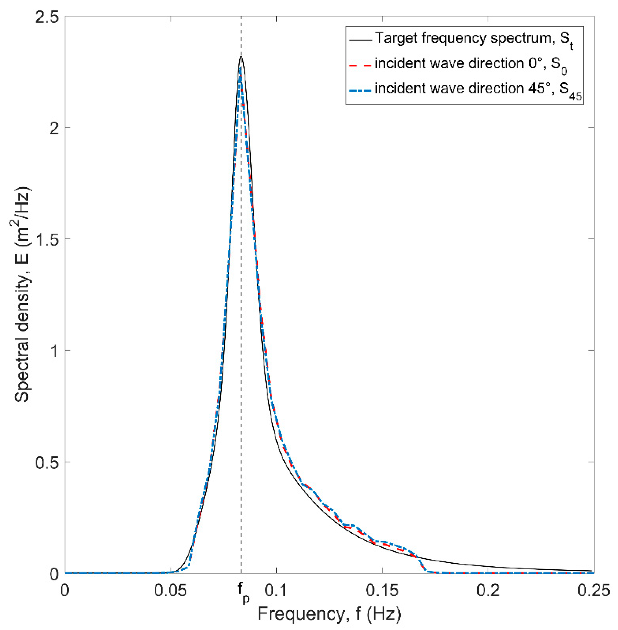
3.2. Generation of Irregular Long Crested Waves

We consider a test case of uni-directional irregular waves fitting a JONSWAP spectrum, with a peak wave period, ${\mathrm{T}}_{\mathrm{p}}$ = 12 s, a significant wave height, ${\mathrm{H}}_{\mathrm{s}}$ = 1 m, and a peak enhancement factor, $\mathsf{\gamma }$ = 3.3. The frequency range is confined between 0.75 ${\mathrm{f}}_{\mathrm{p}}$ and 2 ${\mathrm{f}}_{\mathrm{p}}$, which covers 94% of the total energy, to ensure numerical stability. Periodic lateral boundaries are applied at the top and bottom of the domain similar to Section 3.1, while the length of the sponge layers at both ends of the numerical basin is determined by the longest wave length in the incident wave spectrum. The grid cell size and the time step, $\mathsf{\Delta }\mathrm{t}$, are defined by considering the highest frequency (2 ${\mathrm{f}}_{\mathrm{p}}$) and the lowest frequency (0.75 ${\mathrm{f}}_{\mathrm{p}}$), respectively.

A single wave generation line is placed at the left boundary after the sponge layer. To obtain a steady state wave field, time series of the surface elevation of irregular waves are generated for a duration of 7200 s with a time step of $\mathsf{\Delta }\mathrm{t}$ = 0.2 s. Figure 7 shows the plan views of the ${\mathrm{k}}_{\mathrm{d}}$ values and the water surface elevations in an inner domain (part of the domain without the left and right sponge layers) of 1 km in both directions, at a time instant of $\mathrm{t}$ = 7000 s, for wave propagation angles of $\mathsf{\theta }$ = 0° and $\mathsf{\theta }$ = 45°. It is clear that for both wave propagation angles, the ${\mathrm{k}}_{\mathrm{d}}$ is uniform all over the inner domain with values close to ${\mathrm{k}}_{{\mathrm{d}}_{\mathrm{t}}}$ = 1. In addition, it is observed by comparing the surface elevation of the two different wave directions that for the case of $\mathsf{\theta }$ = 45°, the surface is not as uniform along the crest as it is for the case of $\mathsf{\theta }$ = 0°. This is happening due to the fact that in order to ensure that waves are periodic, the wave propagation angle, $\mathsf{\theta }$, of each wave component is slightly adjusted and a directional spread of the wave energy occurs as described in detail in Section 2.2. Hence, the wave propagation angle varies from 43.2° to 47.7° for the present wave conditions. However, the deviation from the mean wave direction is small and the waves can be considered as uni-directional.

In Figure 8, a comparison is made between the target frequency spectrum (${\mathrm{S}}_{\mathrm{t}}$) and the simulated frequency spectra (${\mathrm{S}}_0$ and ${\mathrm{S}}_{45}$) for the cases of $\mathsf{\theta }$ = 0° and $\mathsf{\theta }$ = 45°. The surface elevations, $\mathsf{\eta }$, at the electronic wave gauges, which are positioned at the centre of the computational domain, are recorded from $\mathrm{t}$ = 40 ${\mathrm{T}}_{\mathrm{p}}$ to $\mathrm{t}$ = 600 ${\mathrm{T}}_{\mathrm{p}}$ with a sampling interval of 0.2 s. The recorded data are processed in segments of 2048 points per segment. A taper window and an overlap of 20% are applied for smoother and statistically more significant spectral estimates. The resulting frequency spectra agree well with ${\mathrm{S}}_{\mathrm{t}}$ apart from those that correspond to wave frequencies higher than 2 ${\mathrm{f}}_{\mathrm{p}}$, since there is no energy for these frequencies in the MILDwave model. Furthermore, it is observed that the periodic lateral boundaries do not affect the waves since for both wave propagation angles, the frequency spectra are similar.

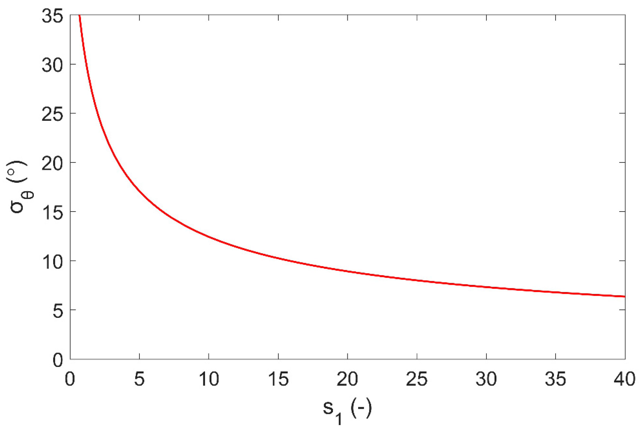
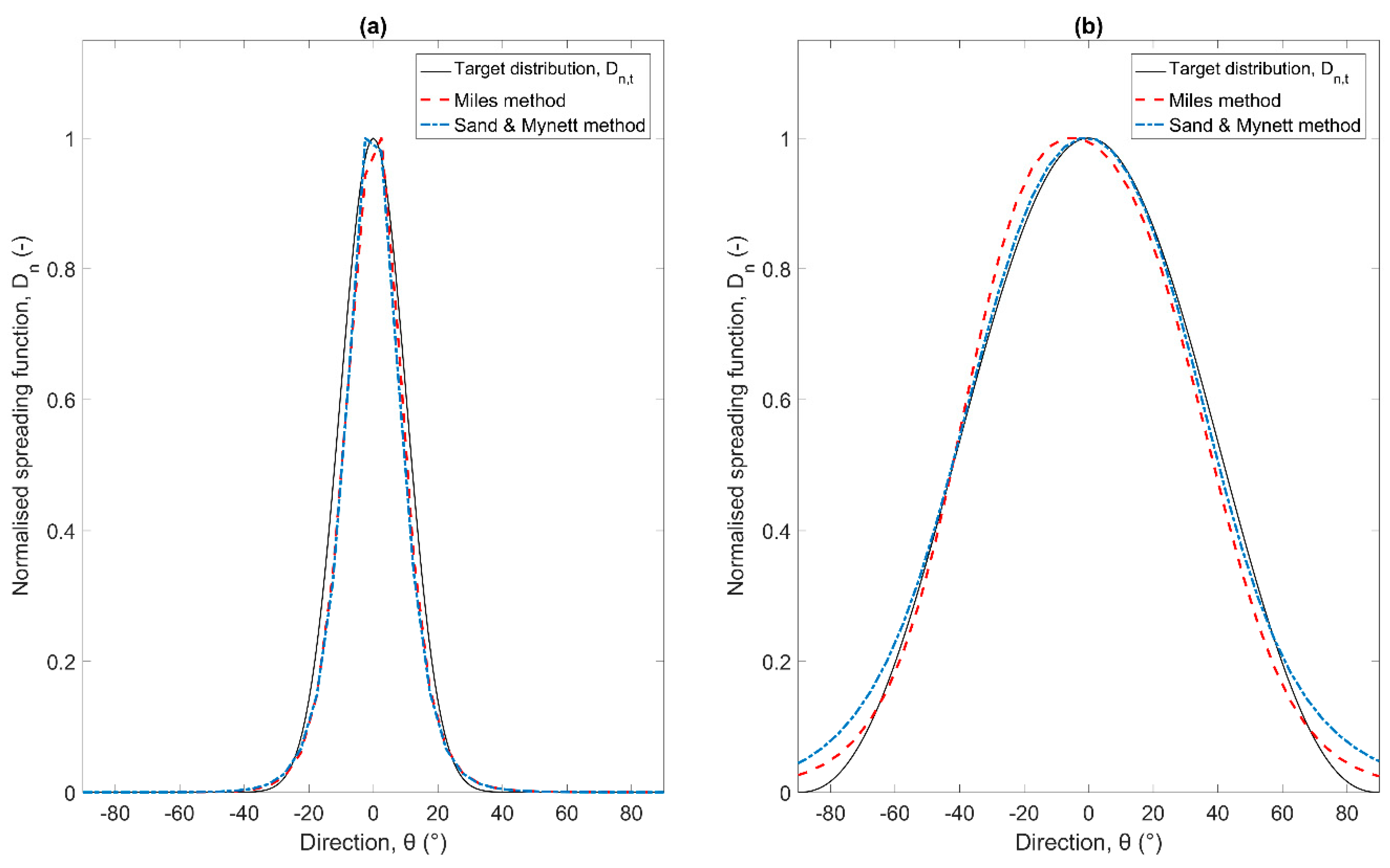
3.3. Generation of Irregular Short Crested Waves

Finally, we consider a test case of irregular short crested waves. The parameters of the input frequency spectrum are identical as for the long-crested irregular waves (${\mathrm{H}}_{\mathrm{s}}$ = 1 m, ${\mathrm{T}}_{\mathrm{p}}$ = 12 s, $\mathsf{\gamma }$ = 3.3) described in the previous section. Waves are generated for a duration of 7200 s with $\mathsf{\Delta }\mathrm{t}$ = 0.2 s while to generate short crested waves, two different wave synthesis methods have been employed: A method proposed by [14] and a method proposed by [15] as described in detail in Section 2.1.

The directional wave spectrum was measured by a group of five wave gauges placed in the centre of the computational domain, using a “CERC 5” configuration as introduced by [29]. The recorded normalised spreading function distributions, ${\mathrm{D}}_{\mathrm{n}}$, are compared with the target distribution, ${\mathrm{D}}_{\mathrm{n},\mathrm{t}}$, in Figure 9 for both wave synthesis methods and for the spreading standard deviation, ${\mathsf{\sigma }}_{\mathsf{\theta }}$ = 10° (swell waves) and ${\mathsf{\sigma }}_{\mathsf{\theta }}$ = 30° (wind waves). The normalised spreading function is calculated by integrating the calculated 3D spectrum over all wave frequencies and normalizing it. The difference between the two measured normalised spreading function distributions of the two methods is small and the agreement with the target distribution is very good. The Sand and Mynett method agrees slightly better with the target distribution, ${\mathrm{D}}_{\mathrm{n},\mathrm{t}}$, than the Miles method especially for the case of ${\mathsf{\sigma }}_{\mathsf{\theta }}$ = 30°.

Figure 10 and Figure 11 show the plan views of the ${\mathrm{k}}_{\mathrm{d}}$ values throughout the inner computational domain and the surface elevations at a time instant of $\mathrm{t}$ = 7000 s for each wave synthesis method for a mean wave propagation angle of $\mathsf{\theta }$ = 0° and spreading standard deviation of ${\mathsf{\sigma }}_{\mathsf{\theta }}$ = 10° and ${\mathsf{\sigma }}_{\mathsf{\theta }}$ = 30°. The results are presented in an inner domain with dimensions of 10 ${\mathrm{L}}_{\mathrm{p}}\times$ 10 ${\mathrm{L}}_{\mathrm{p}}$, where ${\mathrm{L}}_{\mathrm{p}}$ is the wave length that corresponds to the peak wave frequency, ${\mathrm{f}}_{\mathrm{p}}$. It is clear that the Sand and Mynett method yields a more homogenous wave field than the Miles method. Specifically, the maximum (${\mathrm{E}}_{\max }$) value of the calculated absolute errors for the Miles method is 0.051 for ${\mathsf{\sigma }}_{\mathsf{\theta }}$ = 10° and 0.085 for ${\mathsf{\sigma }}_{\mathsf{\theta }}$ = 30°, respectively, while for the Sand and Mynett method, ${\mathrm{E}}_{\max }$ is 0.013 for ${\mathsf{\sigma }}_{\mathsf{\theta }}$ = 10° and 0.029 for ${\mathsf{\sigma }}_{\mathsf{\theta }}$ = 30°, respectively. It is worth mentioning that in the Sand and Mynett method, the number of wave components, ${\mathrm{N}}_{\mathrm{tot}}$, is equal to the number of wave frequencies, $\mathrm{N}$. This is happening due to the fact that the wave propagation angles are randomly selected according to the cumulative distribution function of the directional spreading function, $\mathrm{D}\left(\mathrm{f},\mathsf{\theta }\right)$, and are assigned to each wave frequency component. In contrast to that, in the Miles method, the number of the wave components, ${\mathrm{N}}_{\mathrm{tot}}$, is equal to the product of the number of wave frequencies, $\mathrm{N}$, multiplied with the number of wave angles, $\mathrm{M}$. Thus, in the Sand and Mynett method, (i) the computational time, (ii) the number of corrections of the wave propagation angles in order to ensure the periodicity of the waves, and (iii) the non-homogeneity of the generated wave field are much smaller than those for the Miles method, making the Sand and Mynett method preferable when periodic lateral boundaries are applied in a mild-slope wave model. Specifically, the developed model simulation time for a test case of short crested waves of a duration of 7200 s in a numerical basin, which is 2 km long and 2 km wide, is approximately 3 min on a PC with an Intel Core CPU (Central Processing Unit) 2.90 GHz.

The results show that the MILDwave model with the addition of the periodic boundaries is capable of reproducing a homogeneous short-crested wave field in the whole computational domain as well as the target frequency spectrum and the target directional spectrum. Thus, in future studies, a WEC farm and its effect on the near and far field can be examined under real sea waves by coupling the developed model with a wave-structure interaction solver as described in [19,20]. More precisely, during this coupling methodology, firstly, the short-crested wave field is calculated by the developed model at the position of the WEC farm. Subsequently, this wave field (time series of surface elevation) is used as an input for a wave-structure interaction solver to simulate the diffracted and radiated wave field generated by the presence of the WEC farm. Finally, the resulting wave field is coupled back to MILDwave and propagates throughout the whole numerical domain. As a result, with the coupling methodology in MILDwave, the impact of WEC farms, especially the far field, can be studied using accurate real sea waves.

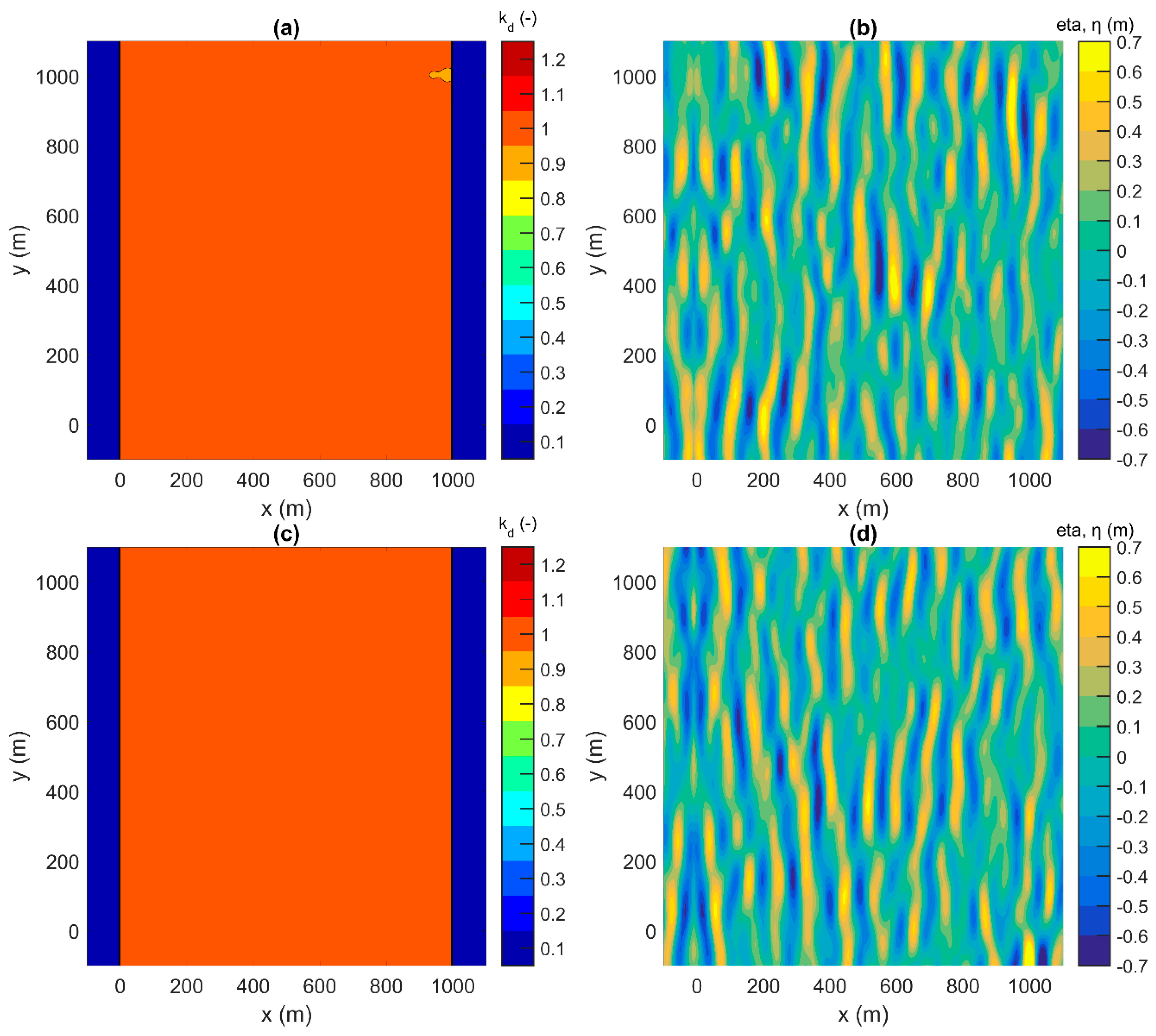
4. Numerical Validation Using the Vincent and Briggs Shoal Experiment

To demonstrate the strategic importance of periodic boundaries in the generation of a short crested wave field over varying water depths, simulations are conducted for waves propagating over a shoal. A study of regular and irregular wave propagation over an elliptic shoal, which has been performed by [30], is used here for validation of the present numerical model.

The bathymetry of the experimental setup of Vincent and Briggs is implemented in MILDwave, as is illustrated in Figure 12, is defined as:

$${\left(\frac{\mathrm{x}}{3.05}\right)}^2+{\left(\frac{\mathrm{y}}{3.96}\right)}^2=1$$

(23)

$${\mathrm{d}}_{\mathrm{e}}=-0.4572+0.7620{\left\{1-{\left(\frac{\mathrm{x}}{3.81}\right)}^2+{\left(\frac{\mathrm{y}}{4.95}\right)}^2\right\}}^{0.5}$$

(24)

where $\mathrm{x}$ and $\mathrm{y}$ are the coordinates centered at the center of the shoal and ${\mathrm{d}}_{\mathrm{e}}$ is the bottom level at any point inside the shoal area. The shoal is similar to that used in the experiments of [31], with a minimum water depth of ${\mathrm{d}}_{\min }$ = 15.24 cm at the center of the shoal while the area around the shoal has a constant water depth of $\mathrm{d}$ = 45.72 cm. In addition, the simulated shoal is located at the center of the numerical domain to take advantage of the lateral periodic boundaries and create a fully developed wave field at the region of the shoal. The grid cell size is $\mathsf{\Delta }\mathrm{x}=\mathsf{\Delta }\mathrm{y}=$ 0.05 m. To obtain a steady state wave field, waves are generated with a duration of 400 s with a time step of $\mathsf{\Delta }\mathrm{t}$ = 0.01 s.

The experiments of Vincent and Briggs are conducted for three kinds of incident breaking and non-breaking waves, i.e., regular, irregular long crested, and irregular short crested waves. In the present study, only irregular long and short crested waves, where large scale breaking is not involved, are examined. The experimental and numerical input wave parameters for non-breaking series are listed in

Table 1. Numerical input wave conditions for non-breaking waves based on the Vincent and Briggs experimental wave conditions.

Test Case ID	$\mathbf{Peak}\mathbf{Period},{\mathbf{T}}_{\mathbf{p}}\left(\mathbf{s}\right)$	$\mathbf{Significant}\mathbf{Wave}\mathbf{Height}{\mathbf{H}}_{\mathbf{s}}\left(\mathbf{cm}\right)$	Phillips Constant, α (-)	Peak Enhancement Factor, γ (-)	Spreading Standard Deviation, σθ (°)
U3	1.3	2.54	0.00155	2	0
N3	1.3	2.54	0.00155	2	10
B3	1.3	2.54	0.00155	2	30
U4	1.3	2.54	0.00047	20	0
N4	1.3	2.54	0.00047	20	10
B4	1.3	2.54	0.00047	20	30

.

Following [30], we use the TMA spectrum [32] as the target wave frequency spectrum in which the spectral energy density, $\mathrm{S}\left(\mathrm{f}\right)$, depends on the parameters, $\mathsf{\alpha }$ (Phillip’s constant), ${\mathrm{f}}_{\mathrm{p}}$ (peak wave frequency), $\mathsf{\gamma }$ (peak enhancement factor), and $\mathsf{\sigma }$ (spectral width parameter), as described in Section 2.1. The parameter, $\mathsf{\gamma }$, is assigned values of 2 for the broad frequency spectrum and 20 for the narrow frequency spectrum. Similarly, these frequency spectra are combined with narrow (${\mathsf{\sigma }}_{\mathsf{\theta }}$ = 10°) and broad (${\mathsf{\sigma }}_{\mathsf{\theta }}$ = 30°) directional spreading, while the $\mathsf{\alpha }$ value is selected to correspond to the target wave height.

The directional spreading function, $\mathrm{D}\left(\mathrm{f},\mathsf{\theta }\right)$, given in Equation (15) is used instead of the wrapped normal spreading function used by [30]. However, the directional spreading parameter, ${\mathrm{s}}_1$, is calculated according to Equation (17) in order to achieve the same distribution as the experimental one. Finally, the mean wave propagation angle is $\mathsf{\theta }$ = 0° and the number of wave components, N, varies from 50 to 400, with the highest value for the case of broad-banded directional spreading. The measured frequency spectra are compared with the target spectrum (${\mathrm{S}}_{\mathrm{t}}$) in Figure 13 for the two values of the peak enhancement factors used here (see Table 1). The agreement is very good especially for the narrow banded spectrum where the measured one replicates the desired target spectrum.

Figure 14 shows the comparison of normalised wave heights, $\mathrm{H}/{\mathrm{H}}_0$, (where $\mathrm{H}$ is the local significant wave height and ${\mathrm{H}}_0$ is the significant wave height at the wave generation boundary) between numerical model results and experimental data along the measurement transect shown in Figure 12 for the test cases of non-breaking waves listed in Table 1. Additionally, to evaluate the model, the root mean square error (RMSE) and the skill factor for the normalised wave heights are calculated as:

$$\begin{array}{cc}\mathrm{RMSE}=\sqrt{\frac{{{\displaystyle \sum }}_{\mathrm{i}=1}^{\mathrm{N}}{\left({\mathrm{P}}_{\mathrm{i}}-{\mathrm{O}}_{\mathrm{i}}\right)}^2}{\mathrm{N}}}& \mathrm{Skill}=1-\sqrt{\frac{{{\displaystyle \sum }}_{\mathrm{i}=1}^{\mathrm{N}}{\left({\mathrm{P}}_{\mathrm{i}}-{\mathrm{O}}_{\mathrm{i}}\right)}^2}{{{\displaystyle \sum }}_{\mathrm{i}=1}^{\mathrm{N}}{\mathrm{O}}_{\mathrm{i}}{}^2}}\end{array}$$

(25)

where $\mathrm{O}$ and $\mathrm{P}$ indicate the observed and predicted values, respectively.

Very good agreement between the numerical model and the experimental model is observed (Figure 14 and

Table 2. Root mean square error (RMSE) and skill factor of the normalised wave heights.

Test Case ID	U3	N3	B3	U4	N4	B4
RMSE	0.141	0.048	0.068	0.068	0.102	0.070
Skill	0.869	0.955	0.936	0.940	0.905	0.924

). MILDwave with the addition of the periodic boundaries correctly predicts the wave focusing behind the shoal for the case of irregular long crested waves where the wave height is strongly affected by the change of the water depth. The model gives a maximum normalised wave height of around 2.05 at y = 0 for both the broad frequency spectrum (Test Case U3) and the narrow frequency spectrum (Test Case U4). On the other hand, a broad directional spreading distribution (Test Case B3, Test Case B4) yields much less spatial wave height variation and the effect of wave refraction is significantly diminished.

5. Conclusions

In the present paper, periodic lateral boundaries were developed in a time dependent mild-slope equation model, MILDwave, for the accurate and fast generation of regular and irregular waves in any direction.

Initially, three different wave generation layouts were examined and compared. The first wave generation layout is an L-shaped wave generator, which is composed of two orthogonal lines. The second wave generation layout is an arc-shaped wave generator where two parallel lines are connected to a semicircle. The third wave generation layout consists of a single wave generation line parallel to the y-axis and periodic lateral boundaries. Numerical experiments were conducted for regular waves with wave propagation angles from $\mathsf{\theta }$ = 0° to $\mathsf{\theta }$ = 45°. The results were presented by means of contour plots, in terms of a disturbance coefficient (${\mathrm{k}}_{\mathrm{d}}$) for the calculation domain, allowing easy comparisons between the different layouts. The wave generation layout with the periodic boundaries showed the best results since this layout leads to a homogeneous wave field, which is not disturbed by unwanted wave diffraction patterns in contrast to the other two wave generation layouts.

Then, this wave generation layout was used to simulate irregular long and short crested waves by using two different wave synthesis methods: A method proposed by Miles [14] and a method proposed by Sand and Mynett [15]. The results indicate that the MILDwave model with the addition of the periodic boundaries is capable of reproducing a homogeneous wave field (especially when the Sand and Mynett method is used) as well as the target frequency spectrum and the target directional spectrum. Finally, the developed model was also used to study wave transformation over an elliptic shoal (Vincent and Briggs shoal experiment), where very good agreement was observed between the numerical model and the experimental results. The aforementioned observations indicate that periodic boundaries make the mild-slope wave model, MILDwave, an essential tool to generate multi-directional waves and study their transformation due to its significantly small computational cost and its high numerical stability and robustness.

The next step is to combine the developed model with the coupling methodology described in [19,20] to study a WEC farm under real sea waves, since this paper proves that now MILDwave is able to accurately generate such a kind of wave field.

References

1. Berkhoff, J.C.W. Computation of combined refraction-diffraction. In Proceedings of the Thirteenth Conference on Coastal Engineering, Vancouver, BC, Canada, 10–14 July 1972; pp. 471–490. [Google Scholar] [CrossRef]
2. Radder, A.C. On the parabolic equation method for water-wave propagation. J. Fluid Mech. 1979, 95, 159–176. [Google Scholar] [CrossRef]
3. Copeland, G.J.M. A practical alternative to the “mild-slope” wave equation. Coast. Eng. 1985, 9, 125–149. [Google Scholar] [CrossRef]
4. Radder, A.C.; Dingemans, M.W. Canonical equations for almost periodic, weakly nonlinear gravity waves. Wave Motion 1985, 7, 473–485. [Google Scholar] [CrossRef]
5. Booij, N. A note on the accuracy of the mild-slope equation. Coast. Eng. 1983, 7, 191–203. [Google Scholar] [CrossRef]
6. Suh, K.D.; Lee, C.; Park, W.S. Time-dependent equations for wave propagation on rapidly varying topography. Coast. Eng. 1997, 32, 91–117. [Google Scholar] [CrossRef]
7. Larsen, J.; Dancy, H. Open boundaries in short wave simulations--A new approach. Coast. Eng. 1983, 7, 285–297. [Google Scholar] [CrossRef]
8. Peregrine, D.H. Long waves on a beach. J. Fluid Mech. 1967, 27, 815–827. [Google Scholar] [CrossRef]
9. Lee, C.; Suh, K.D. Internal generation of waves for time-dependent mild-slope equations. Coast. Eng. 1998, 34, 35–57. [Google Scholar] [CrossRef]
10. Lee, C.; Yoon, S.B. Internal generation of waves on an arc in a rectangular grid system. Coast. Eng. 2007, 54, 357–368. [Google Scholar] [CrossRef]
11. Kim, G.; Lee, C. Internal generation of waves on an arced band. Ocean Eng. 2013, 67, 77–88. [Google Scholar] [CrossRef]
12. Lin, X.; Yu, X. A finite difference method for effective treatment of mild-slope wave equation subject to non-reflecting boundary conditions. Appl. Ocean Res. 2015, 53, 179–189. [Google Scholar] [CrossRef]
13. Troch, P. MILDwave—A Numerical Model for Propagation and Transformation of Linear Water Waves; Internal Report; Department of Civil Engineering, Ghent University: Zwijnaarde, Belgium, 1998. [Google Scholar]
14. Miles, M.D. A Note on Directional Random Wave Synthesis by the Single Summation Method. In Proceedings of the 23rd IAHR Congress, Ottawa, Canada, 21–25 August 1989; pp. 243–250. [Google Scholar]
15. Sand, S.E.; Mynett, A.E. Directional Wave Generation and Analysis. In Proceedings of the IAHR Seminar on Wave Analysis and Generation in Laboratory Basins, Lausanne, Switzerland, 1–4 September 1987; pp. 363–376. [Google Scholar]
16. Troch, P.; Stratigaki, V. Chapter 10—Phase-Resolving Wave Propagation Array Models. In Numerical Modelling of Wave Energy Converters; Folley, M., Ed.; Academic Press: Cambridge, MA, USA, 2016; pp. 191–216. [Google Scholar]
17. Stratigaki, V.; Vanneste, D.; Troch, P.; Gysens, S.; Willems, M. NUMERICAL MODELING OF WAVE PENETRATION IN OSTEND HARBOUR. Coast. Eng. Proc. 2011, 1, 42. [Google Scholar] [CrossRef]
18. Beels, C.; Troch, P.; De Backer, G.; Vantorre, M.; De Rouck, J. Numerical implementation and sensitivity analysis of a wave energy converter in a time-dependent mild-slope equation model. Coast. Eng. 2010, 57, 471–492. [Google Scholar] [CrossRef]
19. Balitsky, P.; Verao Fernandez, G.; Stratigaki, V.; Troch, P. Assessment of the Power Output of a Two-Array Clustered WEC Farm Using a BEM Solver Coupling and a Wave-Propagation Model. Energies 2018, 11, 2907. [Google Scholar] [CrossRef]
20. Verao Fernandez, G.; Balitsky, P.; Stratigaki, V.; Troch, P. Coupling Methodology for Studying the Far Field Effects of Wave Energy Converter Arrays over a Varying Bathymetry. Energies 2018, 11, 2899. [Google Scholar] [CrossRef]
21. Zijlema, M.; Stelling, G.; Smit, P. SWASH: An operational public domain code for simulating wave fields and rapidly varied flows in coastal waters. Coast. Eng. 2011, 58, 992–1012. [Google Scholar] [CrossRef]
22. Shi, F.; Kirby, J.T.; Harris, J.C.; Geiman, J.D.; Grilli, S.T. A high-order adaptive time-stepping TVD solver for Boussinesq modeling of breaking waves and coastal inundation. Ocean Model. 2012, 43–44, 36–51. [Google Scholar] [CrossRef]
23. Brorsen, M.; Helm-Petersen, J. On the Reflection of Short-Crested Waves in Numerical Models. Int. Conf. Coast. Eng. 1998, 394–407. [Google Scholar] [CrossRef]
24. Mitsuyasu, H.; Tasai, F.; Suhara, T.; Mizuno, S.; Ohkusu, M.; Honda, T.; Rikiishi, K. Observations of the Directional Spectrum of Ocean WavesUsing a Cloverleaf Buoy. J. Phys. Oceanogr. 1975, 5, 750–760. [Google Scholar] [CrossRef]
25. Frigaard, P.; Helm-Petersen, J.; Klopman, G.; Stansberg, C.T.; Benoit, M.; Briggs, M.J.; Miles, M.; Santas, J.; Schäffer, H.A.; Hawkes, P.J. IAHR List of Sea Parameteres: an update for multidirectional waves. In Proceedings of the IAHR Seminar Multidirectional Waves and their Interaction with Structures, 27th IAHR Congress, San Francisco, CA, USA, 10–15 August 1997. [Google Scholar]
26. Kuik, A.J.; van Vledder, G.P.; Holthuijsen, L.H. A Method for the Routine Analysis of Pitch-and-Roll Buoy Wave Data. J. Phys. Oceanogr. 1988, 18, 1020–1034. [Google Scholar] [CrossRef]
27. Johnson, D.; Pattiaratchi, C. Boussinesq modelling of transient rip currents. Coast. Eng. 2006, 53, 419–439. [Google Scholar] [CrossRef]
28. Dimakopoulos, A.S.; Dimas, A.A. Large-wave simulation of three-dimensional, cross-shore and oblique, spilling breaking on constant slope beach. Coast. Eng. 2011, 58, 790–801. [Google Scholar] [CrossRef]
29. Borgman, L.E.; Panicker, N.N. Design Study for a Suggested Wave Gauge Array off Point Mugu; Technical Report 1–14; Hydraulic Engineering Laboratory, University of California at Berkeley: Berkeley, CA, USA, 1970. [Google Scholar]
30. Vincent, C.L.; Briggs, M.J. Refraction—Diffraction of Irregular Waves over a Mound. J. Waterw. Port Coastal Ocean Eng. 1989, 115, 269–284. [Google Scholar] [CrossRef]
31. Berkhoff, J.C.W.; Booy, N.; Radder, A.C. Verification of Numerical Wave Propagation Models for Simple Harmonic Linear Water Waves. Coast. Eng. 1982, 6, 255–279. [Google Scholar] [CrossRef]
32. Bouws, E.; Günther, H.; Rosenthal, W.; Vincent, C.L. Similarity of the wind wave spectrum in finite depth water: 1. Spectral form. J. Geophys. Res. 1985, 90, 975. [Google Scholar] [CrossRef]
Figure 1. Water surface elevation, η , for regular incident waves with a wave height of H = 1 m, wave period of T = 12 s, and wave propagation angle of θ = 45° affected by diffraction patterns due to the intersection of the two wave generation lines and the interaction with the lateral sponge layers.
Energies 12 00785 g001
Figure 2. Relation between the directional spreading parameter, s 1 , and the spreading standard deviation, σ θ .
Energies 12 00785 g002
Figure 3. Definition sketch of the implemented periodic lateral boundaries.
Energies 12 00785 g003
Figure 4. Definition sketch of three wave generation layouts: (a) L-shaped, (b) arc-shaped, (c) line-shaped with periodic lateral boundaries. Dimensions are expressed in the number of wave lengths, L w = 100 m, which corresponds to a wave period, T = 12 s, and water depth, d = 7.5 m.
Energies 12 00785 g004
Figure 5. Disturbance coefficient, k d , and water surface elevation, η , in the inner computational domain at t = 80   T for regular incident waves with H = 1 m, T = 12 s, and θ = 30° generated by an L-shaped wave generation layout (a,b), an arc-shaped wave generation layout (c,d), and by the use of periodic boundaries (e,f).
Energies 12 00785 g005
Figure 6. (a) Mean ( E mean ) and (b) maximum ( E max ) value of the absolute errors calculated using Equation (22) for each wave generation layout for a range of different incident wave angles, θ .
Energies 12 00785 g006
Figure 7. Disturbance coefficient, k d , and water surface elevation, η , in the inner computational domain at t = 7000 s for irregular long crested waves with H s = 1 m, T p = 12 s, and (a,b) θ = 0° and (c,d)   θ = 45°.
Energies 12 00785 g007
Figure 8. Comparison between the frequency spectra, S 0 and S 45 , resulting from MILDwave simulations for different incident wave angles ( θ = 0° and θ = 45°, respectively), and the target frequency spectrum, S t , for irregular waves with H s = 1 m, T p = 12 s, and γ = 3.3.
Energies 12 00785 g008
Figure 9. Comparison between the normalised spreading function distributions, D n , calculated in MILDwave with the Miles and the Sand and Mynett wave synthesis methods and the target distribution, D n , t , for irregular short crested waves with a spreading standard deviation, σ θ , of (a) 10° and (b) 30°.
Energies 12 00785 g009
Figure 10. Disturbance coefficient, k d , and water surface elevation, η , in the inner computational domain at t = 7000 s for irregular short crested waves with H s = 1 m, T p = 12 s, θ = 0°, and σ θ = 10° synthesized by using the Miles method (a,b) and the Sand and Mynett method (c,d).
Energies 12 00785 g010
Figure 11. Disturbance coefficient, k d , and water surface elevation, η , in the inner computational domain at t = 7000 s for irregular short crested waves with H s = 1 m, T p = 12 s, θ = 0°, and σ θ = 30°, synthesized by using the Miles method (a,b) and the Sand and Mynett method (c,d).
Energies 12 00785 g011
Figure 12. Bottom levels of the experimental setup used by Vincent and Briggs, as it is implemented in the numerical domain in MILDwave.
Energies 12 00785 g012
Figure 13. Comparison between the frequency spectra simulated in MILDwave and the target frequency spectrum for irregular waves with H s = 2.54 cm, T p = 1.3 s, σ θ = 0°, and (a) γ = 2 and (b) γ = 20.
Energies 12 00785 g013
Figure 14. Comparison of normalised wave heights, H / H 0 , between numerical model results (blue solid lines) and experimental data (red circles) along the measurement transect of Figure 12. for the test cases of non-breaking waves of Table 1.
Energies 12 00785 g014