Article

Modelling Load Profiles of Heat Pumps

Forschungsstelle für Energiewirtschaft e. V., 80995 Munich, Germany
*
Author to whom correspondence should be addressed.
Energies 2019, 12(4), 766; https://doi.org/10.3390/en12040766
Submission received: 6 February 2019 / Revised: 18 February 2019 / Accepted: 24 February 2019 / Published: 25 February 2019
(This article belongs to the Special Issue Energy Efficiency in Plants and Buildings 2019)

Abstract

:
Approximately one quarter of energy-related emissions in Germany are caused by the domestic sector. At 81%, the largest share of these emissions is due to heat supply. Many measures are available to reduce these emissions. One of these measures, which is considered to play an important role in many studies, is the replacement of fossil-fired boilers with electric heat pumps. In order to be able to analyse the impact of high penetrations of heat pumps on the energy system, the coefficient of performance (COP) must be modelled with high temporal resolution. In this study, a methodology is presented on how to calculate high-resolution COPs and the electrical load of heat pumps based on thermal load curves and temperature time series. The COP is determined by the reciprocal Carnot factor. Since heat pumps are often designed bivalently due to the cost structure, the methodology described can also be used for evaluating the combination of immersion heater and heat pump (here for the air/water heat pump). As a result the theoretical hourly COPs determined are calibrated with annual performance factors from field tests. The modelled COPs show clear differences. Currently, mostly air source heat pumps are installed in Germany. If this trend continues, the maximum electrical load of the heat supply will increase more than would be the case with higher shares of ground source heat pumps.

1. Introduction

In the course of the German energy system transformation, the energy supply is being restructured with the aim of phasing out nuclear energy and reducing greenhouse gas emissions [1,2]. With the adoption of the Paris Climate Agreement in 2015, almost the entire world community committed itself to a significant reduction in greenhouse gas emissions, thus creating additional momentum for German efforts.
Extrapolation of the historical development of German greenhouse gas emissions shows that a 40% reduction in greenhouse gases by 2020 compared with 1990 will probably not be achieved with the current legal and regulatory framework. While the share of renewable energies in gross electricity consumption rose to 36% by 2017, it stagnated at 5% in transport and around 13% in heat supply [3]. A look at the German emissions balance shows that domestic sector cause around a quarter of energy-related emissions. At 81%, the largest share of these emissions is due to heat supply [4] (see Figure 1).
Various technical and regulatory measures are at hand to abate CO2 emissions in the energy system. These CO2 abatement measures include low-emission supply through renewable energies, the reduction of demand through more efficient technologies and the electrification of heat and transport. The evaluation of these measures with regard to their cost efficiency and their emissions saving potential is fundamentally dependent on the boundary conditions of the surrounding energy system. Simultaneously, the implementation of such measures always leads to a change in the structure of the entire system and thus to a change in the evaluation basis of further measures. Previous studies dealing with CO2 abatement measures in Germany focus either on the static evaluation of individual measures or on the evaluation of target scenarios using energy system models [5,6,7].
The object of the Dynamic and Intersectoral Evaluation of Measures for the cost-efficient Decarbonisation of the Energy System (Dynamis) project [8] is the development of methods which make it possible to evaluate different measures for CO2 abatement regarding their cost efficiency and their saving potential under changing framework conditions of the energy system. In addition to classical technical and economic parameters, the dynamic interactions between the mostly application-side measures and their impact on the energy system are at the centre of the analysis. For this purpose, two optimisation models of the supply side (electricity and gas) were extended by four stock-and-flow models of the final energy sectors (domestic sector, transport, commerce/trade/ services & industry).
An example of the impact of application-side measures on the energy system are electrification measures, which influence the use of power plants and thus the costs and emissions of the supply sector. This highlights the importance of modelling the electrical load in a practice-oriented way.
Electric heat pumps—as representatives of electrification measures—play an important role in many energy system studies analysing the heat supply of the future [6,7,9]. Electric heat pumps use the Carnot process to utilise environmental heat; thus, contributing to the conservation of resources and the reduction of greenhouse gas emissions, particularly in energy systems with a high share of renewable energies in electricity generation. In addition to the evaluation of the emission reduction of the measure, the system costs are a central component of energy system studies. By definition, these include both costs arising within the final energy sector and costs arising in the supply sector. The latter can be caused by the electricity consumption of electric heat pumps by inducing the use and expansion of generation capacities and storage facilities. The electrical load, in turn, depends on the heat demand, the size and the use of the heat storage tank, and the supply or source temperature. In contrast to the studies mentioned above, which use constant COPs over the year and the approximation using manufacturer curves as in [10], this study presents a methodology for modelling the load of heat pumps with hourly COPs.
The calculation of the hourly COP is part of the model of domestic sector (short: SoPHa [11]). Figure 2 shows a schematic overview of this stock-and-flow model. The initial state of the domestic sector defines the starting point of the simulation and describes the status of the sector in 2015. Based on this, the changes (flow) of the sector states (stock) can be described in annual simulations. The sector state describes the quantity structure of buildings, heating systems, household appliances and users that is necessary to calculate the costs, emissions and load profiles of the sector. Due to the high share of total emissions, SoPHa focuses on the heat supply of households.
To quantify the effects of the abatement measures, the difference between the results from the start scenario and the measure scenario is calculated. The initial scenario shows a development path of the sector up to 2050, which extrapolates historical developments and is in line with current legislation and transformation speed. The overall quantity structures for electricity and heat supply are mainly derived from [12]. It thus corresponds to a conservative path that does not achieve the climate targets of the German government [1,2]. Based on this initial scenario, various measure scenarios are defined whose changes in the sector and effects on the energy system are simulated in the sector model. These measure scenarios correspond to a defined implementation of individual measures within a specified period. The methodology described in this publication is one of many preparations for the evaluation of CO2 abatement measures in the Dynamis project which will be published at the end of this year.

2. Materials and Methods

This paper describes the methodology for deriving electrical load curves of heat pumps from thermal demand load curves and ambient air temperature time series. The overall load curve of all German heat pumps complies with various requirements. On the one hand, an hourly resolution is required in order to be able to analyse the impact on the supply sector. This is indicated by the index ‘h’ in the following equations. In addition, temperature time series at Nomenclature des unités territoriales statistiques (NUTS)-3 level are used in order to take into consideration the simultaneity of different climatic regions. NUTS is a hierarchical classification system used to uniquely identify and classify the subdivisions of the Member States of the European Union. NUTS-3 describes the level of districts. The number of districts can vary significantly from one country to another. In Germany for example there are 429 districts whereas in France there are only 101. For the weighting of these temperature time series, a regionalised building model is used, which divides the building stock into 32 representative building categories [11]. In addition, a distinction is made between brine/water and air/water heat pumps, hereinafter referred to as ground source heat pumps (GSHP) and air source heat pumps (ASHP).
Against this background, this chapter describes the modelling of electrical load profiles of heat-led heating systems ( P S Y S , h ) such as air and ground source heat pumps. The following equations refer to bivalent heat pumps, which are supplemented with an electric immersion heater (here ASHP). However, the methodology can also be applied to monovalent systems (here GSHP). The modelling is based on thermal load curves, which—taking into account distribution losses ( Q ˙ S Y S , h )—are divided by a COP ( C O P S Y S , h ) (see Equation (1)):
P S Y S , h = Q ˙ S Y S , h C O P S Y S , h
The thermal load profiles are composed of domestic hot water load profiles according to VDI 6002 and space heating load profiles based on [13]. As described in [14], the space heat load profiles were simulated in TRNSYS® using typical building and user characteristics. The simulations were carried out for the above mentioned representative building categories. These load profiles were made usable by regression analysis for all possible temperature time series. In SoPHa these were applied for the year 2012 [11] and calibrated with the final energy consumption for space heating in the domestic sector in accordance with [15]. The thermal space heat load is modelled for 32 building types in order to represent the building stock in Germany. In addition to the heat demand, there are on average 16% storage and distribution losses, which are also covered by the heating system. These thermal losses occur at pipes of the space heating and hot water distribution system and at heat storage tanks. Accordingly, Q ˙ S Y S , h describes the thermal output to be provided by the heating system. To model the electrical load of ASHP, the thermal output to be generated is divided into the two system components heat pump (HP) and immersion heater (IH) (see Equation (2)):
P S Y S , h = Q ˙ H P , h C O P H P , h + Q ˙ I H , h 1
For this purpose, it is assumed that the heat pump covers 70% ( Q ˙ H P , h ) and the immersion heater 30% ( Q ˙ I H , h ) of the maximum thermal capacity ( Q ˙ S Y S , m a x ) (see Equation (3)). In practice, not the thermal but the electrical power is limited by the power of the compressor. The mapping of this behaviour could be modelled by means of an iterative calculation based on the methodology described. However, since the difference is only marginal, it is assumed that the thermal capacity of the heat pump is limited (see Equation (3)):
Q ˙ i Q ˙ H P , h ;   Q ˙ i = 0.7 · Q ˙ S Y S , m a x   f o r   Q ˙ i   0.7   · Q ˙ S Y S , m a x                   Q ˙ i   f o r   Q ˙ i <   0.7   · Q ˙ S Y S , m a x
The use of the immersion heater depends on the ambient air temperature. Below a certain bivalence temperature, the immersion heater proportionally supplies the heat. According to the methodology presented, this behaviour is simplified and represented by the thermal output, which is approximately reciprocally proportional to the ambient air temperature. Since the heat demand only exceeds 70% of its maximum value in a few hours of the year, the heat pump provides the majority of the annual heat demand with around 95% [16]. The efficiency of the immersion heater is assumed to be constant at 1, which is why the values of Q ˙ I H , h correspond to those of P I H , h . The modelling of the hourly COP of the heat pump C O P H P , h is explained in detail below. The characteristic of this parameter is modelled by the theoretical maximum COP, which is then scaled with values from field tests to obtain a realistic level of the parameter (see Equation (4)):
C O P H P , h = Q ˙ H P , h P H P , h = Q ˙ H P , h P H P ,   t h e o , h   ·   w H P , s e t w H P ,   t h e o .
In [17] the immersion heater supplies a comparable share of thermal energy, which is why the seasonal performance factors ( S P F S Y S , s e t ) described therein are used to calibrate the heat pump’s electricity demand (see Equations (5)–(7)). This S P F S Y S , s e t represents the average of many heat pump systems of the corresponding technology measured in real operation [17]:
W H P , s e t = Q S Y S S P F S Y S , s e t     W I H , s e t
W H P , t h e o = t = 1 8760 P H P , t h e o , h
P H P , t h e o , h = Q ˙ H P , h C O P H P ,   t h e o , h
The theoretical maximum achievable COP is described by the reciprocal value of the Carnot factor ( η C a r n o t ) (see Equation (8)):
C O P = 1 η C a r n o t = T c o n d T c o n d T e v a     T f l T f l T a
The condensation temperature ( T c o n d ) is simplified by using the average flow temperature for space heating and hot water supply ( T f l ). For the evaporation temperature ( T e v a ), historical ambient air temperatures ( T a ) according to [18] at NUTS-3 level are used. Temperature differences caused by heat exchangers are neglected because they only have a minor influence on the temperature spread.
For the bivalent system, it is also taken into account that the heat pump only has to supply the temperature spread proportionally in cold hours and the immersion heater covers the peak load (see Equation (9)):
C O P H P ,   t h e o , h = S H P , h · T f l , h T a , h + T a , h S H P , h · T f l , h T a , h
In addition, the temperature difference T f l , h T a , h is limited to a minimum of 10 K in order to reduce the number of cycles and thus better reflect the realistic operation of the heat pump. The flow temperature ( T f l , h ) is simplified by combining the flow temperature of the space heat ( T f l , s h , h ) and its hourly share ( S s h , h ) resp. the hot water supply ( T f l , h w , h · S h w , h ) (see Equation (10)):
T f l , h = T f l , s h , h · S s h , h + T f l , h w , h · S h w , h
The flow temperature of the domestic hot water is assumed to be a constant 323 K for single family and two family houses and 373 K for multi family houses in accordance with [19]. The flow temperature for space heating is defined based on weather compensation curves according to [20] (see Equation (11)):
T f l , s h , h = 293   K + 293   K T a , m i x , h 1 1 , 3   ·   0.5   +   3.4   ·   q s h q s h , m i n q s h , m a x q s h , m i n
The differentiation according to building categories is based on the space heating demand per square metre ( q s h ). In addition to the current ambient air temperature T a , h , the temperature T a , m i x , h also takes into account its 72-hour weighted average [14]. T a , m i x , h is composed as follows:
T i     T a , m i x , h   ;   T i   =   T a , h   f o r   10   a . m .   t o   4   p . m . T a , 72 h   f o r   5   p . m .   t o   9   a . m .
The procedure described above makes it possible to model the electrical load of the heat pump P H P , h , from which the hourly resolved COP can be calculated C O P H P , h in order to obtain the electrical load of the entire heating system P S Y S , h .

3. Results

This chapter describes the key modelling results using two exemplary building categories. These include temperature spreads, COPs and load profiles. In addition to the results shown here, the same parameters are available for 32 building categories and in hourly resolution for the year 2012 for all NUTS-3 levels in Germany. Extracts of the results for all 32 building categories examined can be found in Table A1.
For the following Figures, the single family house of the construction age class before 1979 (a) and the multi-family house with seven to 12 apartments of the building age class 1995 to 2020 (b) were selected as examples. These building categories have different prerequisites for the use of heat pumps and show how different the results can be for comparable heat demands. The different efficiency of air and ground source heat pumps is also visualised.

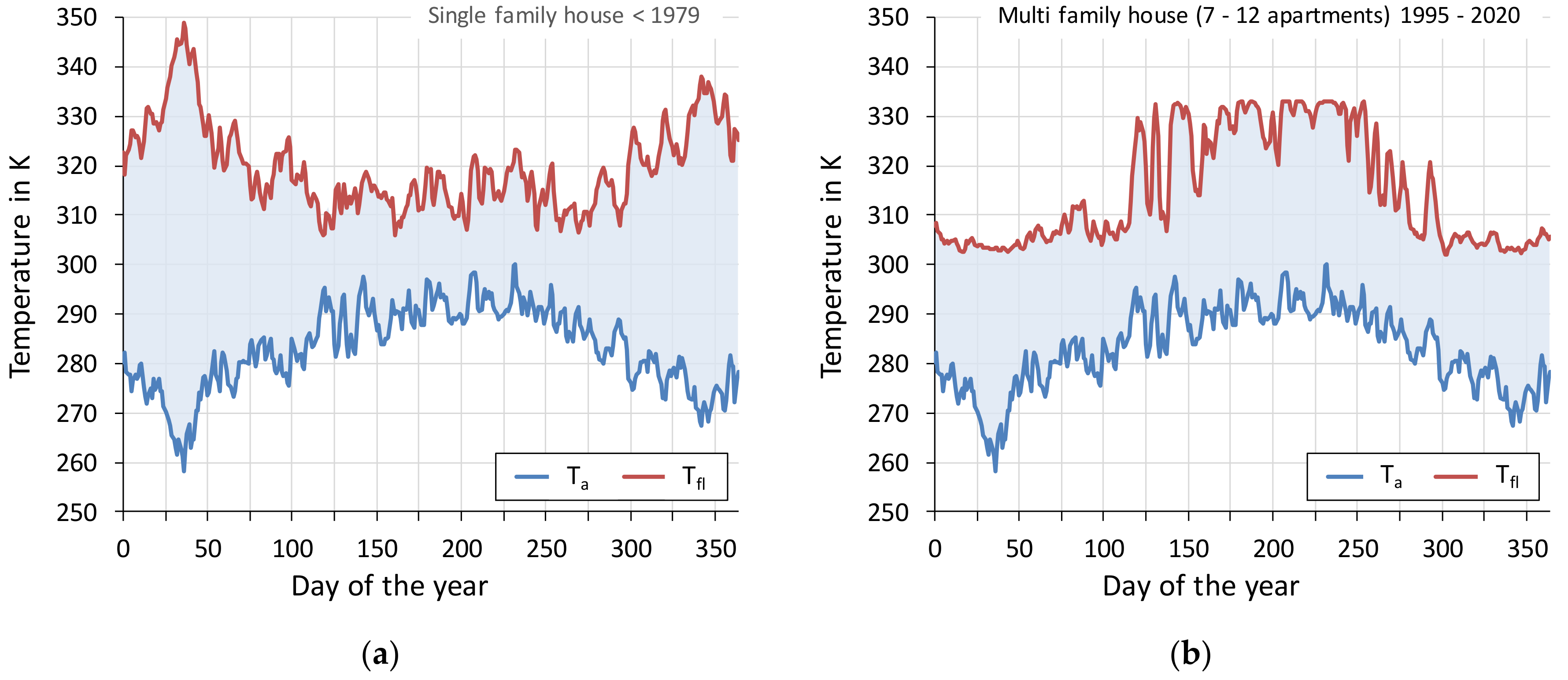
3.1. Temperature Spread—Air Source Heat Pump

The efficiency of heat pumps depends largely on the temperature spread to be provided, which the flow temperature of the heat supply and the source temperature determine. In the case of an ASHP, the source temperature corresponds to the ambient air temperature (Ta). While the ambient air temperature represents an exogenous value, the flow temperature (Tfl) is calculated for each building according to Equation (11). Figure 3 shows the daily mean values of the source and flow temperature of the selected building categories over the year.
The old single family house is characterised by a high share of space heating in the total heat demand (90%) (see Table A1) and shows strong seasonal variations in the flow temperature. In this case, the flow temperature of the space heating is largely responsible for the level of the flow mix temperature (Tfl). Since the old single family house has a large specific heat demand, high flow temperatures must be guaranteed in the heat exchangers in order to be able to supply the space heating demand. In summer, the flow mix temperature is dominated by the supply of hot water.
In contrast to the old single family house, the new multi-family house is characterised by underfloor heating with lower flow temperatures, a higher share of hot water supply in the heat demand (25%) and a higher hot water temperature due to legionella protection (see DIN 1988‑200 and [21]). For these reasons, the flow mix temperature in the new multi-family house is the contrary of that in the old single family house. This results in a temperature spread of the daily mean values of maximum 25 K in the new multi-family house and 78 K in the old single family house.

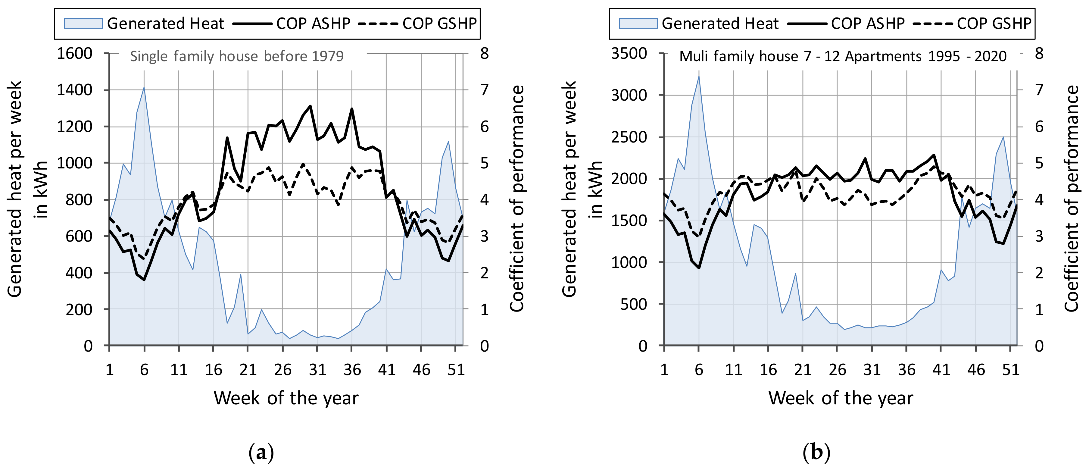
3.2. Coefficient of Performance–Air and Ground Source Heat Pump

This section compares the COP for air and ground source heat pumps using weekly mean values (see Figure 4) for the old single family house (a) and the new multi-family house (b). In contrast to the ASHP, the GSHP can use an almost constant heat source over the course of the year. In the comparison to the ambient air temperature, this is characterised by higher temperatures in the winter and lower temperatures in the summer. As a result, the COP of the GSHP is higher in winter and lower in summer. The weekly mean values of the COP for the GSHP vary from a minimum of 2.4 to a maximum of 5.0, whereas those of the ASHP range from 1.8 to 6.6 (see Figure 4a). The time-resolved COP must be set in relation to the heat demand in order to evaluate the overall efficiency. While the ASHP achieves higher COPs in summer, it has a significantly lower heat demand. In winter, on the other hand, the contrary is the case: the ASHP covers high heat demands with comparatively low COPs. Due to the higher weighting of the COP in winter, the seasonal performance factor of the GSHP (3.3) is higher than that of the ASHP (2.9).
As a result of the higher temperature spread in winter, the COP is lower in single family houses than in multi-family houses (see Figure 4b). In summer, the opposite is true, since the higher share of hot water (see Table A1) in a multi-family house leads to a higher temperature spread.

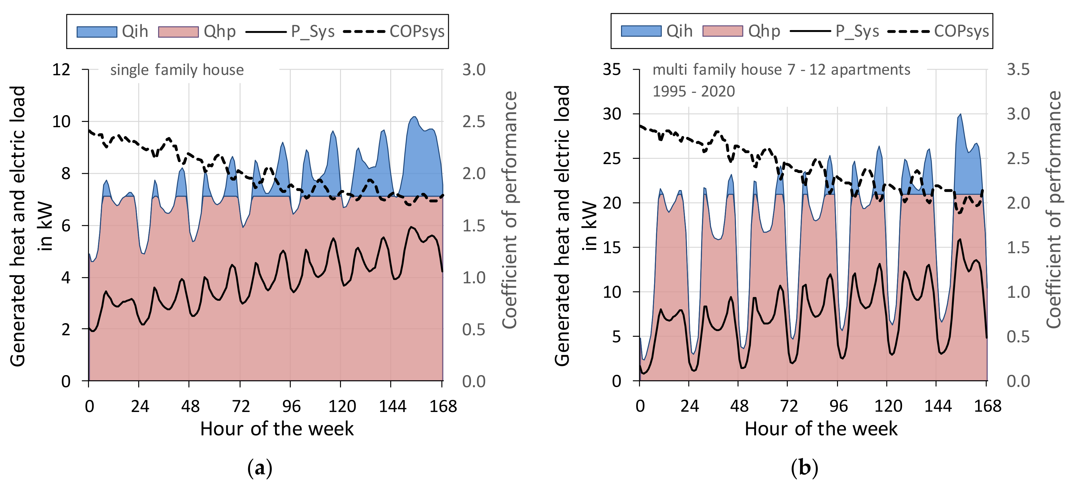
3.3. Thermal and Electrical Load Profile—Air Source Heat Pump

Figure 5 shows the thermal generation (immersion heater and ASHP), the electrical load of the overall system and the COP, each in hourly resolution for the week with the highest heat demand.
A comparison between the old single family house (a) and new multi-family house (b) shows that the thermal generation of the multi-family house has higher gradients. The specific space heating demand of the old single family house at 137 kWh/(m²*a) is significantly higher than that of the multi- family house at 63 kWh/(m²*a). The high specific demand according to [13] already includes the prebound effect. This effect leads to a lower room air temperature in heated rooms and partly unheated rooms. As a result, the average room air temperature during the day is only 289 K. In multi- family houses, on the other hand, this is 294 K during the day due to the rebound effect. As a result the night-time reduction in the single family house considered has a very small effect, whereas in the multi-family house it causes strong changes in the load.
The immersion heater—according to Equation (3)—supplies heat proportionally from the defined thermal output of 7.1 kW resp. 21 kW. In the hour of the maximum annual thermal load, it reaches its maximum value of 3.1 kW resp. 9.0 kW (30% of the heating load). The heat pump supplies a constant thermal capacity during these times. The system COP decreases when the immersion heater is used. The immersion heater achieves a share of 5.6% in the single family house and 3.8% in the multi-family house in the electricity consumption of the heat pump system.
Table 1 lists the minimum, maximum and mean values of characteristic values of the building categories examined. It illustrates the large ranges of values in which the relevant parameters move. For example, the flow temperature in the single family house fluctuates by 55 K, the share of the immersion heater in electricity consumption by 52% and the COP by 820%. Based on these results, high-resolution modelling of the load curve of electric heat pumps to evaluate the impact on the energy system is of great importance.

4. Discussion

The results show how the electrical load of heat pumps depends on technology, source temperature, building type and building age. On this basis, the Dynamis project analyses scenarios that represent the entire building stock in Germany. For this purpose, simplifications are made with regard to the load of individual systems. These concern the thermal load curve, which takes into account the simultaneity of the presence of residents; the flow temperature, which is assumed to be a simplified mix of hot water and space heating; as well as the assumption that all systems are currently operated in a heat-led mode.
In this way, market penetrations of different technologies and their impact on the energy system can be studied. Current studies suggest that heat pumps should only be installed in renovated or new buildings. In fact, the calculations described in this paper show that uninsulated buildings lead to a lower SPF due to higher flow temperatures of the space heating supply and to a stronger seasonality of the electricity demand. Nevertheless, the models should also be able to simulate heat pumps in uninsulated buildings. On the one hand not only the efficiency of the heat pump but also the related emissions of the electricity demand have to be set in relation to the emissions of the existing heating system (e.g. gas or oil boiler). And on the other hand the renovation of significant parts of the building stock might lead to higher costs. If the current trend in the expansion of heat pumps continues, the number of heat pumps will rise much more slowly than required by many system studies, and the share of ASHP will continue to rise. The consequence of this is that the maximum electrical load on the heat supply increases more rapidly than would be the case with a higher share of GSHP. Since the maximum load in the electricity grid occurs during the winter months [22], heat pumps make a major contribution to the maximum load in a high-penetration scenario. The resulting costs for the supply of energy and power are the subject of current work in the Dynamis project. Bivalent heating systems such as heat pumps with gas boilers or systems with large heat storage tanks can— assuming they are intelligently controlled—lead to a reduction in the maximum load. In this context, an intelligent control system takes into account not only supply-side parameters such as costs or emissions, but also application-side restrictions such as the heat demand to be supplied and the COP depending on the generation output.

Supplementary Materials

The following are available online at https://www.mdpi.com/1996-1073/12/4/766/s1, Table S1: Thermal load depending on ambient air temperature, building category, hour of day and type of day.

Author Contributions

Conceptualization, J.C.; Data curation, J.C.; Formal analysis, J.C.; Funding acquisition, J.C.; Investigation, J.C.; Methodology, J.C. and S.G.; Project administration, J.C.; Resources, J.C. and S.G.; Software, J.C.; Supervision, J.C.; Validation, J.C. and S.G.; Visualization, J.C.; Writing—original draft, J.C.; Writing—review & editing, S.G.

Funding

This research was funded by Bundesministerium für Wirtschaft und Energie, grant number 03ET4037A and the following 12 companies: Bayernwerk AG, BMW Group, EnBW Energie Baden-Württemberg AG, Evonik Technology & Infrastructure GmbH, EWE AG, innogy SE, LEW Lechwerke AG, Main-Donau Netzgesellschaft mbH, NuCellSys GmbH, rhenag Rheinische Energie AG, Stadtwerke Rosenheim GmbH & Co. KG, Uniper Kraftwerke GmbH.

Conflicts of Interest

The authors declare no conflict of interest.

Appendix A

Table A1. Analysed COPs of the simulated building categories and their characteristic values.
BuildingBuilding Age ClassRenovation LevelQsh
in kWh/a
Qhw
in kWh/a
Living Space
in m²
COP
ASHP (Sih)
COP
GSHP
Single family house <1979-19,04121601392.9 (5.6%)3.3
partial18,63121601393.0 (4.8%)3.4
full977521601393.3 (4.7%)3.8
1979–1994-15,01724381393.1 (4.6%)3.5
partial14,31524381393.1 (4.8%)3.6
full9,90124381393.3 (4.7%)3.8
1995–2020-10,61524701393.3 (4.8%)3.8
2021–2050-228624701393.8 (4.1%)4.4
Multi-family house <7 apartments<1979-37,02555973103.1 (4.5%)3.5
partial33,45755973103.1 (4.9%)3.6
full19,49955973103.4 (4.7%)3.9
1979–1994-29,34560233103.2 (4.2%)3.7
partial25,29360233103.3 (5.0%)3.8
full19,46660233103.4 (4.9%)3.9
1995–2020-21,52162513103.3 (4.5%)3.8
2021–2050-491562513103.8 (3.3%)4.4
Multi-family house 7–12 apartments<1979-65,86611,6275893.1 (4.8%)3.6
partial48,86611,6275893.3 (5.0%)3.8
full30,12111,6275893.5 (4.7%)4.0
1979–1994-52,38812,9205893.2 (4.7%)3.7
partial36,47212,9205893.4 (4.6%)4.0
full30,84312,9205893.5 (4.3%)4.0
1995–2020-37,08212,5175893.4 (3.8%)3.9
2021–2050-957312,5175893.8 (3.7%)4.4
Multi-family house >12 apartments<1979-143,08827,87413983.2 (4.7%)3.6
partial102,56427,87413983.4 (4.9%)3.9
full66,46327,87413983.5 (4.0%)4.1
1979–1994-117,79328,61513983.3 (3.8%)3.8
partial84,34928,61513983.4 (4.2%)4.0
full66,87728,61513983.5 (4.3%)4.1
1995–2020-79,11322,84513983.4 (3.3%)4.0
2021–2050-18,46722,84513983.8 (3.1%)4.5

References

  1. Ein neuer Aufbruch für Europa Eine neue Dynamik für Deutschland Ein neuer Zusammenhalt für unser Land—Koalitionsvertrag zwischen CDU, CSU und SPD 19; Legislaturperiode: Berlin, Germany, 2018.
  2. Climate Action Plan 2050—Principles and Goals of the German Government’s Climate Policy; Federal Ministry for the Environment, Nature Conservation, Building and Nuclear Safety: Berlin, Germany, 2016.
  3. Zeitreihen zur Entwicklung der Erneuerbaren Energien in Deutschland unter Verwendung von Daten der Arbeitsgruppe Erneuerbare Energien-Statistik (AGEE-Stat); Umweltbundesamt, Fachgebiet I 2.5—Energieversorgung und -daten: Dessau-Roßlau, Germany, 2018.
  4. Rasch, M.; Regett, A.; Pichlmaier, S.; Conrad, J.; Greif, S.; Guminski, A.; Rouyrre, E.; Orthofer, C.; Zipperle, T. Eine Anwendungsorientierte Emissionsbilanz—Kosteneffiziente und Sektorenübergreifende Dekarbonisierung des Energiesystems in BWK; Verein Deutscher Ingenieure (VDI): Düsseldorf, Germany, 2017; Volume 03/2017, pp. 38–42. [Google Scholar]
  5. Kosten und Potenziale der Vermeidung von Treibhausgasemissionen in Deutschland—Eine Studie von McKinsey & Company, Inc., Erstellt im Auftrag von “BDI Initiativ—Wirtschaft und Klimaschutz”; BDI Bundesverband der Deutschen Industrie e.V.: Berlin, Germany, 2007.
  6. Gerhardt, N.; Sandau, F.; Scholz, A.; Hahn, H.; Schumacher, P.; Sager, C.; Bergk, F.; Kämper, C.; Knörr, W.; Kräck, J.; Lambrecht, U.; et al. Interaktion EE-Strom, Wärme und Verkehr—Analyse der Interaktion zwischen den Sektoren Strom, Wärme/Kälte und Verkehr in Deutschland in Hinblick auf steigende Anteile fluktuierender Erneuerbarer Energien im Strombereich unter Berücksichtigung der Europäischen Entwicklung; Fraunhofer-Institut für Windenergie und Energiesystemtechnik: Berlin, Germany, 2015. [Google Scholar]
  7. Kruse, J.; Hennes, O.; Wildgrube, T.; Lencz, D.; Hintermayer, M.; Gierkink, M.; Peter, J.; Lorenczik, S. Dena-Leitstudie Integrierte Energiewende—Teil B; ewi Energy Research & Scenarios gGmbH: Köln, Germany, 2018; p. 26. [Google Scholar]
  8. Conrad, J.; Fattler, S.; Regett, A. Ongoing Project: Dynamis—Dynamic and Intersectoral Evaluation of Measures for the Cost-Efficient Decarbonisation of the Energy System; Research Center for Energy Economics: Munich, Germany, 2016; Available online: https://www.ffe.de/en/783 (accessed on 9 January 2017).
  9. Langenheld, A.; Mellwig, P.; Pehnt, M.; von Oehsen, A.; Blömer, S.; Lempik, J.; Werle, M.; Ganal, I.; Gerhardt, N.; Becker, S.; et al. Wert der Effizienz im Gebäudesektor in Zeiten der Sektorenkopplung; Agora Energiewende: Berlin, Germany, 2018. [Google Scholar]
  10. Verhelst, C.; Logist, F.; Van Impe, J.; Helsen, L. Study of the optimal control problem formulation for modulating air-to-water heat pumps connected to a residential floor heating system. Energy Build. 2012, 45, 43–53. [Google Scholar] [CrossRef]
  11. Conrad, J.; Greif, S. Modelling the private households sector and the impact on the energy system. In Proceedings of the 41st IAEE Conference, Groningen, The Netherlands, 10–13 June 2018. [Google Scholar]
  12. Schlesinger, M.; Lindenberger, D.; Lutz, C. Development of Energy Markets—Energy Reference Forecast—Projekt Nr. 57/12; Federal Ministry of Economics and Technology: Berlin, Germany, 2014. [Google Scholar]
  13. Stratou, E. Auswirkung der Energetischen Gebäudequalität auf den Wärmelastgang von Wohngebäuden—Abbildung Mittels Repräsentativer Typologien und Baualtersklassen. Master’s Thesis, Technische Universität München and Forschungsstelle für Energiewirtschaft e.V., Munich, Germany, 2018; p. 76. [Google Scholar]
  14. Greif, S.; Conrad, J.; Schmid, T. Methoden zur Erstellung Synthetischer Wärmelastgänge. et—Energiewirtschaftliche Tagesfragen—Zeitschrift für Energiewirtschaft, Recht, Technik und Umwelt; EW Medien und Kongresse GmbH: Berlin, Germany, 2018; Volume 10, pp. 23–25. [Google Scholar]
  15. Energy Data: Complete Edition; Federal Ministry for Economic Affairs and Energy: Berlin, Germany, 2016.
  16. Recknagel, H.; Sprenger, E.; Schramek, E.R. Recknagel—Taschenbuch für Heizung + Klimatechnik; Karl-Joseph Albers: Munich, Germany, 2016; Volume 78. [Google Scholar]
  17. Günther, D.; Miara, M.; Langner, R.; Helmling, S.; Wapler, J. WP Monitor—Feldmessung von Wärmepumpenanlagen; Fraunhofer-Institut für Solare Energiesysteme (ISE): Freiburg, Germany, 2014; p. 104. [Google Scholar]
  18. Weather Data of the DWD; Deutscher Wetterdienst (DWD): Offenbach, Germany, 2014; Available online: https://webservice.dwd.de/cgi-bin/spp1167/webservice.cgi (accessed on 6 December 2018).
  19. Arbeitsblatt W 551—Trinkwassererwärmungs- und Trinkwasserleitungsanlagen; Technische Maßnahmen zur Verminderung des Legionellenwachstums; Planung, Errichtung, Betrieb und Sanierung von Trinkwasser-Installationen; DVGW Deutsche Vereinigung des Gas- und Wasserfaches e.V.: Bonn, Germany, 2004.
  20. Tischer, L. Installation Rules and Guidelines; Robur S.p.A.: Verdellino, Italy, 2014. Available online: https://slideplayer.com/slide/10888512/ (accessed on 14 February 2019).
  21. Kleinertz, B.; Dufter, C.; Greif, S.; Conrad, J. Energieeinsparpotenziale Durch die Optimierung Bestehender Trinkwassersysteme—Betrachtung von Mietwohnungen und Einfamilienhäusern mit Zentralem und dezentralem System; Forschungsstelle für Energiewirtschaft e.V.: Munich, Germany, 2017. [Google Scholar]
  22. Conrad, J.; von Roon, S. Beitrag Elektrischer Heizsysteme zur Jahreshöchstlast im Deutschen Übertragungsnetz in: Energiewirtschaftliche Tagesfragen; etv Energieverlag GmbH: Essen, Germany, 2014. [Google Scholar]
Figure 1. Emissions caused by domestic sector in 2014 (temperature adjusted).
Energies 12 00766 g001
Figure 2. Schematic overview of the stock-and-flow model of domestic sector.
Energies 12 00766 g002
Figure 3. Ambient air temperature (Ta) and floor temperature (Tfl) of an air source heat pump in a single family house of the building age class before 1979 (a) and a multi-family house with seven to 12 apartments of the building age class 1995 to 2020 (b).
Energies 12 00766 g003
Figure 4. Comparison of the COP and the generated heat of an air source heat pump and a ground source heat pump for a single family house before 1979 (a) and a multi-family house of the building age class 1995–2020 (b).
Energies 12 00766 g004
Figure 5. Generated heat, electric load and COP of an air source heat pump system in a single family house before 1979 (a) and a multi family house of the building age class 1995–2020 (b).
Energies 12 00766 g005
Table 1. Characteristic values for air source heat pumps in the two building categories analysed.
Building TypeParameterMinMaxAverage
Single family house
<1979
ta in K256308283
tfl in K297352320
COPSYS1.7142.9
SIH_el0%52%6%
PSYS in kW0.06.11.0
Multi family house
7–12 apartments
2021–2050
tfl in K256308283
COPSYS2.16.93.8
SIH_el0%66%4%
PSYS in kW0.08.80.8

