A Continuation Power Flow Model of Multi-Area AC/DC Interconnected Bulk Systems Incorporating Voltage Source Converter-Based Multi-Terminal DC Networks and Its Decoupling Algorithm

Abstract

Existing continuation power flow (CPF) models mainly focus on the regional independent systems, which are not suitable for multi-area AC/DC interconnected systems because the market trading behaviors and security control for power allocation of tie-lines are ignored. This study presents a novel CPF model and its decoupling algorithm for multi-area AC/DC interconnected systems incorporating a voltage source converter (VSC)-based multi-terminal direct current (MTDC) network. This CPF model includes the following unique features: (1) In view of the bilateral power trading contracts among regional subsystems, the nonlinear constraint equations of directional trading active power via interface are derived, and the multi-balancing machine strategy is introduced to realize the active power balance of each subsystem. (2) An accurate simulation method for the security control behaviors of the power allocation in tie-lines is proposed, which includes a specific selection strategy for automatic generation control units and a generation re-dispatch strategy. These two strategies work together to prevent the serious overload in tie-lines during load growth and improve the voltage stability margin of the interconnected bulk systems. (3) The switching characteristic of reactive power control behaviors of VSC stations is simulated in the CPF calculation. In the end, a novel decoupling CPF algorithm based on bi-directional iteration is presented to realize the decomposition and coordination calculation. This decoupling algorithm preserves the precision and convergence of integrated CPF algorithms, and it has an apparent advantage on the calculation speed. Furthermore, this decoupling algorithm also can easily reflects the effects of the control mode changes of VSC stations to the voltage stability margin of AC system. Case studies and comparative analysis on the IEEE two-area RTS-96 system indicate the effectiveness and validity of the proposed CPF model and corresponding decoupling algorithm.

1. Introduction

As a basic tool for static voltage stability analysis of power system, the continuation power flow (CPF) method has been widely used in the security analysis and it has become a core function in the energy management systems [1,2]. With the continuous development of electrical technology, the modern power system already has the characteristics of multi-area AC/DC interconnection [3], long-distance bulk power transmission, and large-scale renewable energy connection [4].

Under this new situation, the voltage source converter (VSC)-based multi-terminal direct current (MTDC) transmission network becomes a highly potential optimal scheme for interconnected tie-lines [3,5,6], because of its features of active and reactive powers that can be controlled independently [7], immunization to commutation failure, and easy to extend to multi-terminal networks [8]. Most studies about VSC-MTDC focus on the steady-state power flow model [7,8,9,10], electromechanical stability [11,12] and control strategies [13,14,15,16], while related researches in the field of CPF are very few [17,18,19]. In reference [17], the continuous parameter at the present operation point is determined by an integrated prediction calculation firstly, and then an AC/DC power flow algorithm based on alternating iterations will update the values of state variables. The effect of different VSC controlling values on the voltage stability margin (VSM) is also discussed in [17]. Reference [18] derived the computational formula for sensitivities of the load margin with respect to the active and reactive power control parameters of VSCs. Based on the above sensitivities, an adjustment strategy for the control parameter values is introduced. However, the corresponding studies in the field of CPF cannot reflect the switching characteristics of reactive power control behaviors of the VSC stations during the load growth.

Most recent research conducted in the field of CPF has focused on the problem of poor condition at the saddle-node bifurcation point [20,21,22] and the nonlinear effect of varying parameters, such as transmission branch parameters [23,24] and power injections [25]. Nevertheless, all existing studies are for the independent regional grid, and little attention is paid to the market trading behaviors and the power limitation of tie-lines in the interconnected systems. The voltage stability margin (VSM) calculated by the CPF model can evaluate the maximum load increment in the interconnected systems correctly only by fully considering the influence of the bilateral power trading contracts (BPTC) among regional subsystems and accurately simulating the power control behaviors of tie-lines.

The current AC/DC interconnected bulk systems still have the following problems that need to be solved when the CPF method is applied:

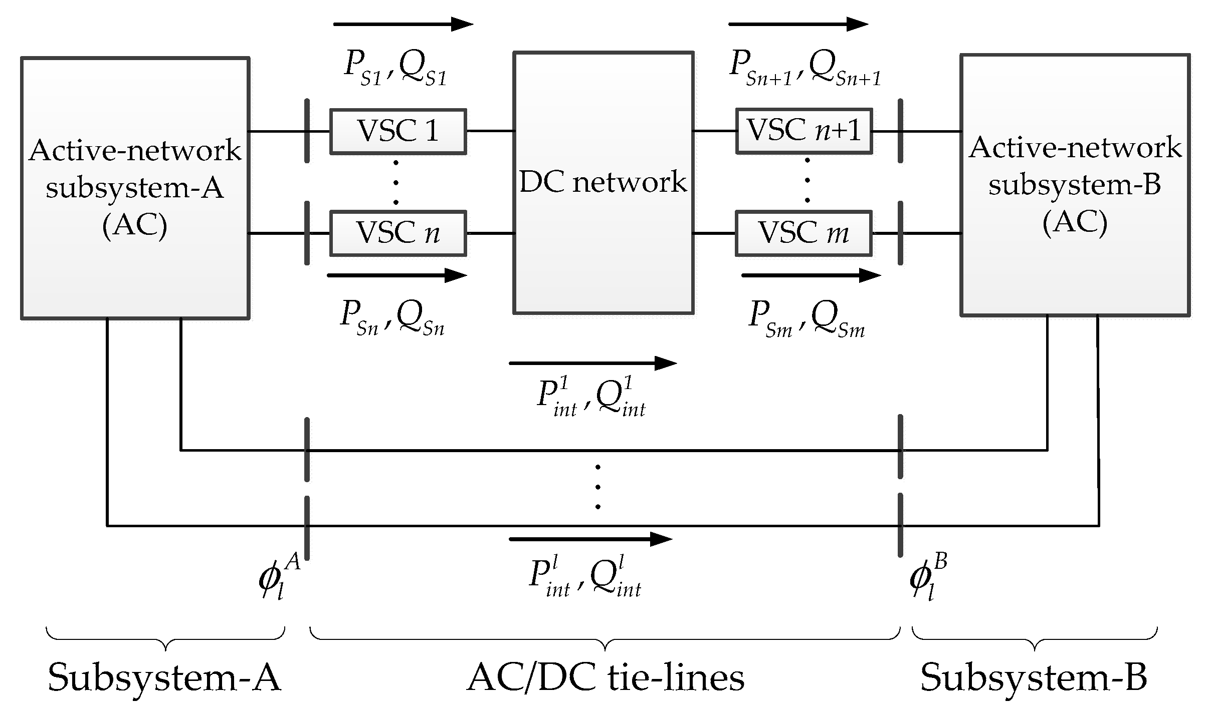
1. Simulation for the influence of BPTC on VSM

In the electricity market environment, the directional trading active power (DTAP) transmitted between interconnected subsystems is determined using the BPTC and it cannot be changed during the contract period even if the inner power flow of subsystems varies. This limitation is an essential difference between the interconnected bulk systems and the independent regional grid. However, this issue is neglected in the existing literatures on CPF.

The automatic generation control (AGC) system is usually installed in the dispatching and control centers of each subsystem. With the real-time adjustment of AGC system, the total DTAP via the interconnected interface can approximate the predefined set value. Accurately simulating the control behaviors of AGC units is difficult when the CPF model that considers BPTC is established.

2. Security control for power allocation of tie-lines

Multiple transmission tie-lines are usually between subsystems, and the power allocation of tie-lines is determined by the impedance of branches and power injections. When the power injections change unevenly, under the constraint of keeping the total active power transmitted via the interface constant, the power allocation proportion of tie-lines will change considerably. In extreme situations, serious overload or severe unbalanced power distribution in tie-lines may occur. Therefore, in actual interconnected systems, the total balance of active power via the transmission interface should be guaranteed. Moreover, the selected AGC units or even the units participating in the distribution of load increment should not affect the power transfer security of tie-lines.

The variation of the power allocation of tie-lines is ignored in existing CPF models, which only focus on independent grid or simply render the tie-lines to be equal to the constant PQ load. This negligence will introduce a significant deviation in the calculation of VSM.

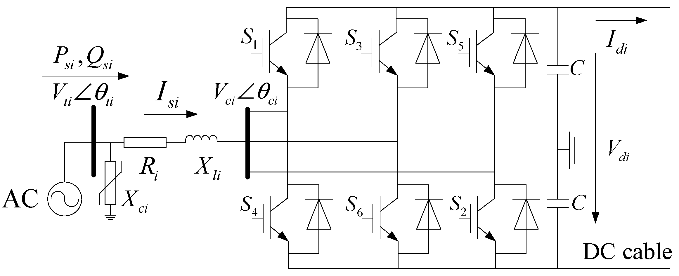
3. Simulation for switching characteristics of reactive power control behaviors of VSC stations

The ability of VSC converter to independently control the reactive power results in two different representations in the power flow algorithms, namely constant reactive power injection $Q_{\mathit{si}}$ into AC grid and the constant AC bus voltage magnitude $V_{\mathit{ti}}$ [8]. Therefore, the PQ or PV mode is usually used to represent the reactive power control behaviors of VSCs in most power flow models on VSC-MTDC [26,27]. The switching characteristics of reactive power control behaviors of VSC stations should be considered during the load growth. For example, when the PQ mode is initially adopted, the voltage magnitude of the AC bus connecting to the VSC will decrease gradually with the load increase in the AC network. Once the voltage magnitude is below the lower security limit, the control mode of the VSC should be switched from PQ to PV mode. Similarly, when the PV mode is adopted during load growth and the reactive power injection into the AC grid exceeds its maximum adjustment range, the control mode of the VSC should be switched from PV to PQ mode. Accurately simulating the switching characteristics of reactive power control behaviors of VSC stations is a key problem to be solved in CPF models.

To address the three aforementioned problems, the present work proposes a novel CPF model for multi-area AC/DC interconnected bulk systems incorporating VSC-MTDC network (herein, M-AC/VSC-MTDC systems). In view of the influence of BPTC among regional subsystems, the nonlinear constraint equations of DTAP via the interface are derived, and a multi-balancing machine strategy is introduced to realize the active power balance of each subsystem. An accurate simulation method, which includes a specific selection strategy for AGC units and a generation re-dispatch strategy, is proposed to simulate the security control behaviors of the power allocation of tie-lines for avoiding serious overload or severe unbalanced power distribution of tie-lines during load growth. Furthermore, the VSC-MTDC network is considered in the proposed CPF model, and a specific switching strategy for VSC controlling modes is developed to simulate the actual reactive power control behaviors of the VSC-MTDC network. All loads are assumed to increase simultaneously for the sake of emphasizing the study’s focus.

In order to solve the proposed CPF model, a novel decoupling CPF algorithm based on bi-directional iteration is also presented to realize the decomposition and coordination calculation between AC systems and DC systems. The characteristics of this decoupling algorithm are summarized as follows: (1) The decomposition and coordination process of AC and DC systems are based on strictly equivalent linear transformation, hence, this decoupling algorithm can preserve the precision and convergence of integrated CPF algorithms. (2) This decoupling CPF algorithm simplifies the hybrid AC/DC prediction equation and correction equation, eliminates 6/7 DC variables, therefore it has an apparent advantage on the calculation speed by comparing with the integrated algorithms. (3) This decoupling algorithm can easily reflects the effects of the control mode changes of VSC stations to the voltage stability margin of AC system. With the proposed decoupling algorithm, when the control modes of VSC stations change, only several coefficient matrices that represent the interaction between the AC system and DC system should be altered, and the prediction equation and correction equation of AC system are not required to be modified.

The remainder of this paper is organized as follows. In Section 2, the power flow model for the VSC-MTDC and the nonlinear constraint equations of DTAP are derived. Section 3 elaborates the proposed CPF model for M-AC/VSC-MTDC interconnected systems. Section 4 describes the decoupling algorithm for the proposed CPF model. In Section 5, five schemes are tested on the IEEE two-area RTS-96 system. The simulations, comparisons, and analysis indicate the effectiveness and validity of the proposed CPF model and decoupling algorithm. Finally, Section 6 concludes the paper.

2. Power Flow Model For M-AC/VSC-MTDC Interconnected Systems

2.1. Power Flow Model for the VSC-MTDC Network

For the power flow modelling of a VSC-MTDC, the following assumptions are adopted:

(1)

Supply voltages are sinusoidal and balanced which contain only fundamental frequency and positive sequence component.

(2)

The harmonics generated by the converters are neglected.

(3)

The switches are assumed to be ideal.

Figure 1 shows the steady-state physical model of a conventional VSC-MTDC network, which consists of multi-bridge converters, converting reactors, AC filters, DC capacitors, and DC cables. Normally, the AC bus that connects directly to the converter is called the point of common coupling (PCC) [12].

To express the model conveniently, the following variable symbols are defined. ${\mathit{VSC}}_i$ refers to the ith VSC. For the ${\mathit{VSC}}_i$, $\overline{V_{\mathit{ti}}}$ is the voltage vector of the PCC bus; $\overline{V_{\mathit{ci}}}$ is the line voltage vector of the converter bridge output; ${\delta }_i$ is the difference of the above two phase angle, ${\delta }_i{=\theta }_{ti}-{\theta }_{\mathit{ci}}$; $X_{\mathit{li}}$ and $X_{\mathit{ci}}$ are the reactance of the converter reactor and AC filter, respectively; $R_i$ is the equivalent resistance that represents the active power loss of the converter bridge; $P_{\mathit{si}}$ and $Q_{\mathit{si}}$ are the active and reactive power injection from the AC network into the ${\mathit{VSC}}_i$, respectively; $V_{\mathit{di}}$ is the output DC voltage of ${\mathit{VSC}}_i$; and $I_{\mathit{di}}$ is the DC current injecting into the MTDC grid.

For the power flow modeling of the VSC-MTDC network, when harmonics generated by the converters are neglected, the power injection into ${\mathit{VSC}}_i$ can be expressed as:

$$P_{\mathit{si}}{+\mathit{jQ}}_{\mathit{si}}=\overline{V_{\mathit{ti}}}{\left[\left(\overline{V_{\mathit{ti}}}-\overline{V_{\mathit{ci}}}\right)/\left(R_i{+\mathit{jX}}_i\right)\right]}^{*}$$

(1)

With the pulse width modulation (PWM) technology, $V_{\mathit{ci}}$ is determined by $V_{\mathit{di}}$, modulation modes, and modulation ratio $M_i$ ($0\le M_i\le 1$) [13,28,29]:

$$V_{\mathit{ci}}{=\mu }_i{M}_i{V}_{\mathit{di}}/\sqrt{2}$$

(2)

where ${\mu }_i$ refers to the utilization rate of DC voltage, which depends on the modulation modes of PWM. When the sinusoidal PWM is used, ${\mu }_i=\sqrt{3}/2$; conversely, ${\mu }_i=1$ when the space vector PWM is applied.

The admittance and admittance angle of $X_{\mathit{li}}$ and $R_i$ are $Y_i$ and ${\alpha }_i$, respectively, which can be expressed as:

$$Y_i=1/\sqrt{R_i^2+X_{\mathit{li}}^2}$$

(3)

$${\alpha }_i=\arctan \left(R_i{/X}_{\mathit{li}}\right)$$

(4)

Substituting (2)–(4) to (1) yields:

$$\{\begin{array}{l}{P}_{\mathit{si}}-\frac{1}{\sqrt{2}}{\mu }_i{M}_i{V}_{\mathit{ti}}{V}_{\mathit{di}}{Y}_i\mathit{sin}\left({\delta }_i-{\alpha }_i\right)-V_{\mathit{ti}}^2{Y}_i{\mathit{sin}\alpha }_i=0\\ Q_{\mathit{si}}+\frac{1}{\sqrt{2}}{\mu }_i{M}_i{V}_{\mathit{ti}}{V}_{\mathit{di}}{Y}_i\mathit{cos}\left({\delta }_i-{\alpha }_i\right)-V_{\mathit{ti}}^2{Y}_i{\mathit{cos}\alpha }_i-V_{\mathit{ti}}^2{X}_{\mathit{ci}}=0\end{array}$$

(5)

The active power loss of the converter bridge is represented by $R_i$; thus, the DC power injection into the DC cables equals the active power injection into the converter bridge. This active power balance can be expressed as:

$$V_{\mathit{di}}{I}_{\mathit{di}}-\frac{1}{\sqrt{2}}{\mu }_i{M}_i{V}_{\mathit{ti}}{V}_{\mathit{di}}{Y}_i\mathit{sin}\left({\delta }_i{+\alpha }_i\right)+\frac{1}{2}{\mu }_i^2{M}_i^2{V}_{\mathit{di}}^2{Y}_i{\mathit{sin}\alpha }_i=0$$

(6)

For the MTDC grid, $g_{\mathit{dij}}$ is the cable conductance between DC bus i and j, and $n_c$ is the number of DC buses. The power flow constrained equation of the DC grid can be expressed as:

$$I_{\mathit{di}}-{\displaystyle \sum }_{j=1}^{n_c}{g}_{\mathit{dij}}{V}_{\mathit{dj}}=0$$

(7)

A total of four associated state variables (i.e., $V_{\mathit{di}}$, $V_{\mathit{ti}}$, $P_{\mathit{si}}$, $Q_{\mathit{si}}$) are in ${\mathit{VSC}}_i$, wherein two of them should be set as the control objectives. The active power injection of VSC stations can be modeled in three different ways: constant active power injection $P_{\mathit{si}}$ mode, constant DC voltage $V_{\mathit{di}}$ mode [8] and the DC voltage droop mode [13,30]. For the DC voltage droop mode, the relationship between $P_{\mathit{si}}$ and $V_{\mathit{di}}$ can be shown as:

$$V_{\mathit{di}}{I}_{\mathit{di}}-P_{\mathit{si}}^{\mathit{sp}}-\frac{V_{\mathit{di}}^{\mathit{max}}-V_{\mathit{di}}^{\mathit{min}}}{P_{\mathit{si}}^{\mathit{max}}-P_{\mathit{si}}^{\mathit{min}}}\left(V_{\mathit{di}}-V_{\mathit{di}}^{\mathit{sp}}\right)=0$$

(8)

where $P_{\mathit{si}}^{\mathit{sp}}$ and $V_{\mathit{di}}^{\mathit{sp}}$ are the specified values of active power injection and DC voltage, respectively; $V_{\mathit{di}}^{\mathit{max}}$ and $V_{\mathit{di}}^{\mathit{min}}$ are the upper and lower limited value of DC voltage, respectively; $P_{\mathit{si}}^{\mathit{max}}$ and $P_{\mathit{si}}^{\mathit{min}}$ are the maximum and minimum active power capacity of the VSC i, respectively.

Similarly, the reactive power injection of VSC can be represented in two different ways: constant $Q_{\mathit{si}}$ mode and constant $V_{\mathit{ti}}$ mode.

The following six combinations are commonly used: (1) constant $V_{\mathit{di}}$ and $Q_{\mathit{si}}$ control; (2) constant $V_{\mathit{di}}$ and $V_{\mathit{ti}}$ control; (3) constant $P_{\mathit{si}}$ and $Q_{\mathit{si}}$ control; and (4) constant $P_{\mathit{si}}$ and $V_{\mathit{ti}}$ control; (5) DC voltage droop mode and constant $Q_{\mathit{si}}$ control; (6) DC voltage droop mode and constant $V_{\mathit{ti}}$ control. The generalized control equations of converters can be expressed as:

$$C_i\left(V_{\mathit{di}},V_{\mathit{ti}},P_{\mathit{si}}{,Q}_{\mathit{si}}\right)=0$$

(9)

2.2. Power Flow Constraints of AC Buses

The AC buses include two types, namely, the inner AC buses ${\phi }_{\mathit{AC}}$ and the PCC buses ${\phi }_{\mathit{PCC}}$. The power flow constrained equations of the AC buses are expressed as:

$$\{\begin{array}{c}{V}_i{{\displaystyle \sum }}_{j\in i}{V}_j\left(G_{\mathit{ij}}{\mathit{cos}\theta }_{\mathit{ij}}{+B}_{\mathit{ij}}{\mathit{sin}\theta }_{\mathit{ij}}\right)-P_{\mathit{gi}}{+P}_{\mathit{di}}=0\\ V_i{{\displaystyle \sum }}_{j\in i}{V}_j\left(G_{\mathit{ij}}{\mathit{sin}\theta }_{\mathit{ij}}-B_{\mathit{ij}}{\mathit{cos}\theta }_{\mathit{ij}}\right)-Q_{\mathit{gi}}+Q_{\mathit{di}}=0\end{array},i\in {\phi }_{\mathit{AC}}$$

(10)

$$\{\begin{array}{c}{V}_i{{\displaystyle \sum }}_{j\in i}{V}_j\left(G_{\mathit{ij}}{\mathit{cos}\theta }_{\mathit{ij}}{+B}_{\mathit{ij}}{\mathit{sin}\theta }_{\mathit{ij}}\right)-P_{\mathit{gi}}{+P}_{\mathit{di}}{+P}_{\mathit{si}}=0 \\ V_i{{\displaystyle \sum }}_{j\in i}{V}_j\left(G_{\mathit{ij}}{\mathit{sin}\theta }_{\mathit{ij}}-B_{\mathit{ij}}{\mathit{cos}\theta }_{\mathit{ij}}\right)-Q_{\mathit{gi}}{+Q}_{\mathit{di}}{+Q}_{\mathit{si}}=0\end{array},i\in {\phi }_{\mathit{PCC}}$$

(11)

where $P_{\mathit{gi}}$ and $Q_{\mathit{gi}}$ are the active and reactive output of the generator at bus i, respectively; and $P_{\mathit{di}}$ and $Q_{\mathit{di}}$ are the load at bus i.

2.3. Nonlinear Constraint Equations of DTAP via Interface and the Multi-Balancing Machine Strategy

In this study, the multi-area interconnected system is assumed to be synchronous, in which the tie-lines include several AC and DC lines. Figure 2 shows the schematic of the AC/VSC-MTDC interconnected structure. The interconnected systems consist of three parts, that is, the AC active networks (subsystem-A and -B), the DC tie-line network (an m-terminal DC transmission grid), and the AC tie-line network (l AC tie-lines).

In the electricity market, the bilateral active power contracts among regional subsystems are enforceable. The nonlinear constraint equations of DTAP via interface can be expressed as:

$$\begin{array}{c}{\displaystyle \sum }_{jϵ{\phi }_l^A,k\in {\phi }_l^B}{P}_{\mathit{jk}}^l+{\displaystyle \sum }_{iϵ{\phi }_{\mathit{PCC}}^A}{P}_{\mathit{si}}-P_{\mathit{ref}}=0\hfill \\ P_{\mathit{jk}}^l=V_j^2{\hat{G}}_{jk}-V_j{V}_k({\hat{G}}_{jk}\mathit{cos}{\theta }_{jk}+{\hat{B}}_{jk}\mathit{sin}{\theta }_{jk})\hfill \end{array}$$

(12)

where ${\phi }_l^A$ and ${\phi }_l^B$ are the terminal buses of the AC tie-lines located in subsystems-A and -B, respectively; ${\phi }_{\mathit{PCC}}^A$ refers to the PCC buses located in subsystem-A; ${\hat{G}}_{jk}$ and ${\hat{B}}_{jk}$ are the conductance and admittance of AC tie-line $l_{\mathit{jk}}$, respectively; and $P_{\mathit{ref}}$ is the specified DTAP transmitted from subsystem-A to subsystem-B.

When the load varies or increases in the interconnected systems, the active power transmitted in the AC and DC tie-lines should be controlled simultaneously to ensure that the total active power transmitted via the interface satisfies the requirements of (12) constantly. For the DC tie-lines, the active power control can be realized by setting the controlling modes of VSCs; whereas for the AC tie-lines, the control of active power via AC interconnected interface can be realized by adjusting the active power output of AGC units in each subsystem. The multi-balancing machine strategy is utilized in this study to simulate the controlling behaviors of AGC units. Particularly, the slack bus ($V\theta$ bus) is set in a major subsystem, of which the voltage vector is given. Simultaneously, a V bus is set in every other subsystem, of which the voltage magnitude is given.

Generally, (5)–(12) form the power flow model of M-AC/VSC-MTDC interconnected systems, and the model can be simply expressed as:

$$\{\begin{array}{l}D\left(V_{\mathit{di}}{,I}_{\mathit{di}}{,\delta }_i{,M}_i{,V}_{\mathit{ti}}{,P}_{\mathit{si}}{,Q}_{\mathit{si}}\right)=0\\ f\left({\mathit{x},P}_{\mathit{si}}{,Q}_{\mathit{si}}\right)=0\\ S\left({\mathit{x},P}_{\mathit{si}}\right)=0\end{array}$$

(13)

where x is the state vector of the AC buses, which includes the voltage amplitudes and voltage phase angles; D(•) represents the power flow model of the VSC-MTDC network, which consists of (5)–(7) and (9); f (•) represents the power flow constraints of the AC buses, which consists of (10) and (11); and S(•) represents the constraint equation of DTAP via interface, that is, (12).

3. CPF Model For M-AC/VSC-MTDC Interconnected Systems

On the basis of the power flow model established in Section 2, the load growth factor λ, the distribution of active power supply, the security control for power allocation of tie-lines, and the switching characteristic of reactive power control behaviors of VSC stations should be further considered when the CPF model for M-AC/VSC-MTDC interconnected systems is established.

3.1. Extended Parameterized Power Flow Equations

The conventional CPF process consists of four basic elements, namely, parameterization, predictor, corrector, and step-length control [31]. Parameterization is the key part of mathematical modeling, which often includes local [21,32], arc-length [31], and orthogonal parameterization [23,33]. Given the quadratic characteristics of the parameterized equation and the large calculation residual, the PV curves can converge rapidly in the upper part of the curve, and diverging near the nose point is difficult when the arc-length parameterization is used. The arc-length parameterization is selected in this study after comprehensive comparison with other parameterized methods.

The active load increment is usually assumed to be distributed by generators according to the proportion of the residual active power capacity of each unit. The parameterized load and output of units can be expressed as:

$$\{\begin{array}{c}{P}_{\mathit{di}}\left(\lambda \right){=P}_{\mathit{di}0}\left({1+\lambda K}_{\mathit{pi}}\right),i\in {\Omega }_d \\ Q_{\mathit{di}}\left(\lambda \right){=Q}_{\mathit{di}0}\left({1+\lambda K}_{\mathit{qi}}\right),i\in {\Omega }_d \\ P_{\mathit{gi}}\left(\lambda \right){=P}_{\mathit{gi}0}{+\Delta P}_{\mathit{gi}}^1\left(\lambda \right),i\in {\Omega }_g \\ {\Delta P}_{\mathit{gi}}^1\left(\lambda \right)={{\displaystyle \sum }}_{jϵ{\Omega }_d}\left({\lambda K}_{\mathit{pj}}{P}_{\mathit{dj}0}\right)\frac{P_{\mathit{reserve},i}}{{{\displaystyle \sum }}_{iϵ{\Omega }_g}{P}_{\mathit{reserve},i}} \end{array}$$

(14)

where λ is the load growth factor; $P_{\mathit{di}0}$ and $Q_{\mathit{di}0}$ are the initial active and reactive load at bus i, respectively; $P_{\mathit{gi}0}$ is the initial active power output of the generator at bus i; $K_{\mathit{pi}}$ and $K_{\mathit{qi}}$ are the active and reactive load growth coefficients at bus i, respectively; $P_{\mathit{reserve},i}$ is the current residual active power capacity of the generator at bus i; and ${\Omega }_d$ and ${\Omega }_g$ are the bus groups of load and generator nodes, respectively.

When the $P_{\mathit{di}}$, $Q_{\mathit{di}}$, and $P_{\mathit{gi}}$ in (13) are replaced with the $P_{\mathit{di}}\left(\lambda \right)$, $Q_{\mathit{di}}\left(\lambda \right)$, and $P_{\mathit{gi}}\left(\lambda \right)$ in (14), respectively, and the arc-length parameterization method [31] is applied, the extended parameterized power flow equation for M-AC/VSC-MTDC interconnected systems can be written as:

$$\{\begin{array}{l}D\left(V_{\mathit{di}}{,I}_{\mathit{di}}{,\delta }_i{,M}_i{,V}_{\mathit{ti}}{,P}_{\mathit{si}}{,Q}_{\mathit{si}}\right)=0\\ f\left({\mathit{x},P}_{\mathit{si}}{,Q}_{\mathit{si}},\lambda \right)=0\\ S\left({\mathit{x},P}_{\mathit{si}}\right)=0\\ w\left(\mathit{x},\lambda \right)={\left(\mathit{x}-{\mathit{x}}_0\right)}^T\left(\mathit{x}-{\mathit{x}}_0\right)+(\lambda -{\lambda }_0{)}^2-{\sigma }^2=0\end{array}$$

(15)

where $w(\mathit{x},\lambda )$ is the arc-length parameterized equation; ${\mathit{x}}_0$ and ${\lambda }_0$ are the state vector and the load growth factor at previous operation point, respectively; and σ refers to the step size.

3.2. Security Control for the Power Allocation of Tie-lines

As mentioned in Section 1, during load growth, the power allocation proportion of tie-lines may change considerably. In extreme situations, such change will result in serious overload or severe unbalanced power distribution of tie-lines. The following strategies can be adopted according to the practice experience:

Strategy-S1: When selecting AGC units, the units that have a deep influence on the power allocation proportion of tie-lines (DIPA units for short) should be excluded.

Strategy-S2: The maximum output of DIPA units should be limited during load growth, and these units should not participate in the distribution of load increment.

Strategies-S1 and -S2 refer to the selection strategy for AGC units and the generation re-dispatch strategy, respectively. The selection of AGC units and the distribution scheme of load increment for an actual operating interconnected system are known in advance. Accordingly, this relevant information should be considered in the CPF calculation. The above information cannot be fully informed for a standard test system. In this situation, the sensitivity group $K_g^l$, which represents sensitivities of the active power transmitted via tie-lines to the active power output of generators, can be calculated on the basis of (13). The detailed calculation progress of $K_g^l$ is as follows:

$$K_g^l=\left\{k_{g,i}^{l,j}|\forall i\in {\Omega }_g,j\in {\Omega }_{\mathit{tiel}}\right\}$$

(16)

$$k_{g,i}^{l,j}=\frac{P_{\mathit{tiel},j}^{\tau }-P_{\mathit{tiel},j}^0}{{\tau P}_{\mathit{gi}0}}$$

(17)

where, $k_{g,i}^{l,j}$ refers to the sensitivity of the active power transmitted via the jth tie-line to the active power output of the generator i; ${\Omega }_g$ and ${\Omega }_{\mathit{tiel}}$ refer to the groups of generators and tie-lines, respectively; $\tau$ refers to a small and constant growth factor of the active power output of generators, and it is set as 0.1 in this paper; $P_{\mathit{gi}0}$ is the initial active power output of generator i; $P_{tiel, j}^0$ refers to the active power transmitted via the tie-line j of the initial power flow state; $P_{\mathit{tiel},j}^{\tau }$ refers to the active power transmitted via the tie-line j when only the active power output of generator i increases by ${\tau P}_{\mathit{gi}0}$. $P_{\mathit{tiel},j}^0$ and $P_{tiel, j}^{\tau }$ can be calculated with the power flow model established in Section 2, namely (13). Then, appropriate AGC units and the generators participating in the distribution of load increment can be determined using the $K_g^l$ and transmission security upper limit of tie-lines.

3.3. Switching Strategy of VSC Controlling Modes

As described in Section 2, in normal circumstances, the converters of VSC-MTDC network usually work on control Mode 1), 3) or 5), and the reactive power injection $Q_{\mathit{si}}$ into VSCs will remain stable. Along with the load increase, if the voltage magnitude of PCC bus $V_{\mathit{ti}}$ is extremely low (e.g., below the threshold value $V_{\mathit{tcr}}$), then the control mode of VSC will convert from Mode 1) to Mode 2), from Mode 3) to Mode 4) or from Mode 5) to Mode 6). Meanwhile, the controlling target switches from constant $Q_{\mathit{si}}$ to constant $V_{\mathit{ti}}$, and the voltage magnitude of PCC bus will be kept as $V_{\mathit{tcr}}$. Similarly, if the VSC has been working under the constant $V_{\mathit{ti}}$ mode and the reactive power injection into VSC exceeds the limits, then the controlling mode of VSC will return to the constant maximum $Q_{\mathit{si}}$ mode.

4. Bi-Directional Iteration Algorithm for the Proposed CPF Model

The proposed CPF model, namely (15) can be divided into two parts: the constraint equations of VSC-MTDC network, which refer to D(•); the constraint equations of AC systems, which consist of f(•), S(•) and $w$(•). By observing the proposed CPF model, the following characteristics can be found:

(1)

The constraint equations of AC and DC systems have common variables $V_{\mathit{ti}}$, $P_{\mathit{si}}$ and $Q_{\mathit{si}}$.

(2)

According to the constraint equations of VSC-MTDC network, when there are n VSC converters, then number of the corresponding constraint equations is 6n, and that of the variables is 7n. The difference between the numbers of equations and variables makes the linear transformation possible.

Based on the above characteristic, a novel decoupling CPF algorithm based on bi-directional iteration is proposed in this section to realize the decomposition and coordination calculation between AC systems and DC systems. For the convenience of description, the variables in DC constraint equations ($V_{\mathit{di}}{,I}_{\mathit{di}}{,\delta }_i{,M}_i{,V}_{\mathit{ti}}{,P}_{\mathit{si}}{\mathrm{and}Q}_{\mathit{si}}$) are defined as DC variables while the variable x in AC constraint equations is defined as AC variable, and the voltage magnitude of PCC bus $V_{\mathit{ti}}$ is chosen as the common coordinated variable shared by above both.

The decoupling calculation process is summarized as follows: Firstly, the forward and backward equations of prediction and correction steps are derived with linear transformation, which represent the interaction between AC systems and DC systems. Secondly, all the other DC variables in the prediction equation and correction equation will be substituted by $V_{\mathit{ti}}$ with corresponding forward equations, then the prediction equation and correction equation only contain AC variable x. Thirdly, the AC variables x at next operation point can be calculated by solving the simplified prediction equation and correction equation. Finally, the DC variables at next operation point can be obtained by the updated $V_{\mathit{ti}}$ with the corresponding backward equations. This iterative calculation process will be continued until the saddle-node bifurcation point reaches. This decoupling algorithm preserves the precision and convergence of integrated CPF algorithms, and it can easily reflects the effects of the control mode changes of VSC stations to the VSM of AC systems.

4.1. The Forward and Backward Equations for the VSC-MTDC System

The main calculation steps of the CPF are prediction and correction [31]. Firstly, for the prediction step, differential calculation is applied on both sides of the power flow constraint equation of VSC-MTDC, namely D(•) in (15). Then the corresponding differential equation of DC system is:

$$\left[\begin{array}{ccc}\frac{\partial D}{\partial X_d}& \frac{\partial D}{\partial P_{\mathit{si}}}& \frac{\partial D}{\partial Q_{\mathit{si}}}\end{array}\right]\left[\begin{array}{c}{\mathit{dX}}_d\\ {\mathit{dP}}_{\mathit{si}}\\ {\mathit{dQ}}_{\mathit{si}}\end{array}\right]+\frac{\partial D}{\partial V_{\mathit{ti}}}{\mathit{dV}}_{\mathit{ti}}=0$$

(18)

where $X_d=\left[V_{\mathit{di}}{,I}_{\mathit{di}}{,\delta }_i{,M}_i\right]$; ${\mathit{dX}}_d$, ${\mathit{dP}}_{\mathit{si}}$, ${\mathit{dQ}}_{\mathit{si}}$ and ${\mathit{dV}}_{\mathit{ti}}$ are the tiny increment of $X_d$, $P_{\mathit{si}}$, $Q_{\mathit{si}}$ and $V_{\mathit{ti}}$, respectively; and the $\left[\partial D/\partial X_d,\partial D/\partial P_{\mathit{si}},\partial D/\partial Q_{\mathit{si}}\right]$ is the coefficient matrix of partial derivatives.

Apply the linear transformation to (18) and eliminate the coefficient matrix, then it can be obtained:

$$\{\begin{array}{c}{\mathit{dP}}_{\mathit{si}}=-J_{\mathit{dPsi}}^P{\mathit{dV}}_{\mathit{ti}}\\ {\mathit{dQ}}_{\mathit{si}}=-J_{\mathit{dQsi}}^P{\mathit{dV}}_{\mathit{ti}}\end{array}$$

(19)

$${\mathit{dX}}_d=-J_{\mathit{dx}}^P{\mathit{dV}}_{\mathit{ti}}$$

(20)

where the $J_{\mathit{dx}}^P$, $J_{\mathit{dPsi}}^P$ and $J_{\mathit{dQsi}}^P$ are the submatrices of coefficient matrix in the prediction obtained by linear transformation. In this paper, the equation (19) is defined as the forward equation of prediction step while (20) is defined as the backward equation of prediction step.

Similarly, for the correction step, when the Taylor series is applied to D(•), and the second and higher order items are ignored, the following correction equation can be derived:

$$\left[\begin{array}{ccc}\frac{\partial D}{\partial X_d}& \frac{\partial D}{\partial P_{\mathit{si}}}& \frac{\partial D}{\partial Q_{\mathit{si}}}\end{array}\right]\left[\begin{array}{c}\Delta X_d\\ \Delta P_{\mathit{si}}\\ \Delta Q_{\mathit{si}}\end{array}\right]+\frac{\partial D}{\partial V_{\mathit{ti}}}\Delta V_{\mathit{ti}}=-\Delta D$$

(21)

where $\Delta X_d$, $\Delta P_{\mathit{si}}$, $\Delta Q_{\mathit{si}}$ and $\Delta V_{\mathit{ti}}$ are the deviations of the variables $X_d$, $P_{\mathit{si}}$, $Q_{\mathit{si}}$ and $V_{\mathit{ti}}$, respectively.

Apply the linear transformation to (21) and eliminate the coefficient matrix of partial derivatives, namely $\left[\partial D/\partial X_d,\partial D/\partial P_{\mathit{si}},\partial D/\partial Q_{\mathit{si}}\right]$, then the following equation can be obtained:

$$\{\begin{array}{c}\Delta P_{\mathit{si}}=-J_{\mathit{dPsi}}^C\Delta V_{\mathit{ti}}-C_{\mathit{Psi}}\\ \Delta Q_{\mathit{si}}=-J_{\mathit{dQsi}}^C\Delta V_{\mathit{ti}}-C_{\mathrm{Qsi}}\end{array}$$

(22)

$${\Delta X}_d=-J_{\mathit{dx}}^C{\Delta V}_{\mathit{ti}}-C_d$$

(23)

where the $J_{\mathit{dx}}^C$, $J_{\mathit{dPsi}}^C$ and $J_{\mathit{dQsi}}^C$ are the submatrices of coefficient matrix in the correction step obtained by linear transformation; $C_d$, $C_{\mathit{Psi}}$ and $C_{\mathrm{Qsi}}$ are the subvectors of the column vector obtained by linear transformation. In this paper, the Equation (22) is defined as the forward equation of correction step while (23) is defined as the backward equation of correction step.

Thus, the Equations (19), (20), (22) and (23) form the forward and backward equations for the VSC-MTDC system. Concretely, the constraint equations of DC variables $X_d$ and $V_{\mathit{ti}}$, namely (20) and (23), reflect the influence of the AC system on DC systems; the constraint equations of power injections into VSC stations and $V_{\mathit{ti}}$, namely (19) and (22), reflect the influence of the DC system on AC system.

4.2. Prediction Step

Once a basic solution has been found (for $\lambda =0$), the next solution can be predicted by taking an appropriately sized step in a direction tangent to the solution path. Appling the Tangent method [21] to the constraint equations of AC network in the proposed CPF model, namely the f(•), S(•) and $w$(•) in (15), then the prediction equation for AC network can be expressed as:

$$\left[\begin{array}{c}\begin{array}{cccc}\frac{\partial f}{\partial P_{\mathit{si}}}& \frac{\partial f}{\partial Q_{\mathit{si}}}& \frac{\partial f}{\partial \mathit{x}}& \frac{\partial f}{\partial \lambda }\\ \frac{\partial S}{\partial P_{\mathit{si}}}& 0& \frac{\partial S}{\partial \mathit{x}}& 0\\ 0& 0& \frac{\partial w}{\partial \mathit{x}}& \frac{\partial w}{\partial \lambda }\end{array}\end{array}\right]\left[\begin{array}{c}{\mathit{dP}}_{\mathit{si}}\\ {\mathit{dQ}}_{\mathit{si}}\\ \mathit{dx}\\ d\lambda \end{array}\right]=\left[\begin{array}{c}0\\ 0\\ \text{±}1\end{array}\right]$$

(24)

It should be emphasized here that $V_{\mathit{ti}}$, as the coordinated variable between AC and DC systems, is part of the state vector x. Substituting (19) to (24) yields:

$$\left[\begin{array}{cc}{H}_P& L_P\\ M_P& 0\\ R_P& S_P\end{array}\right]\left[\begin{array}{c}\mathit{dx}\\ d\lambda \end{array}\right]=\left[\begin{array}{c}0\\ 0\\ \text{±}1\end{array}\right]$$

(25)

where $H_P$, $M_P$, $R_P$, $L_P$ and $S_P$ are the simplified coefficient matrices of prediction step after the substitution. The detailed substitution process and expressions of above coefficient matrices are shown in the Appendix A.

By solving (25), the tiny increment $\mathit{dx}$ and $d\lambda$ can be calculated. Because ${\mathit{dV}}_{\mathit{ti}}$ is part of $\mathit{dx}$, the ${\mathit{dV}}_{\mathit{ti}}$ will be determined once the $\mathit{dx}$ is determined. Substitute ${\mathit{dV}}_{\mathit{ti}}$ into (19) and (20), and then ${\mathit{dP}}_{\mathit{si}}$, ${\mathit{dQ}}_{\mathit{si}}$ and ${\mathit{dX}}_d$ can also be obtained.

Then the prediction will be computed as:

$$\left[\begin{array}{c}{X}_d^{*}\\ P_{\mathit{si}}^{*}\\ Q_{\mathit{si}}^{*}\\ {\mathit{x}}^{*}\\ {\lambda }^{*}\end{array}\right]=\left[\begin{array}{c}{X}_d^{m-1}\\ P_{\mathit{si}}^{m-1}\\ Q_{\mathit{si}}^{m-1}\\ {\mathit{x}}^{m-1}\\ {\lambda }^{m-1}\end{array}\right]+\sigma \left[\begin{array}{c}{\mathit{dX}}_d\\ {\mathit{dP}}_{\mathit{si}}\\ {\mathit{dQ}}_{\mathit{si}}\\ \mathit{dx}\\ d\lambda \end{array}\right]$$

(26)

where superscript $*$ denotes the predicted solution at the present operation point, and superscript $m-1$ demotes the corrected solution at the previous operation point. $\sigma$ refers is a scalar used to adjust the step size.

4.3. Correction Step

The predicted solution obtained by (26) will be regard as the initial value of the extended parameterized power flow equation (15). The Newton-Raphson algorithm is used for iterative calculation until convergence. Use the Taylor series to express the constraint equations of AC network in the proposed CPF model, namely the f(•), S(•) and $w$(•) in (15), and the second and higher order items are neglected. The corresponding correction equations can be described as follows:

$$\left[\begin{array}{c}\begin{array}{cccc}\frac{\partial f}{\partial P_{\mathit{si}}}& \frac{\partial f}{\partial Q_{\mathit{si}}}& \frac{\partial f}{\partial \mathit{x}}& \frac{\partial f}{\partial \lambda }\\ \frac{\partial S}{\partial P_{\mathit{si}}}& 0& \frac{\partial S}{\partial \mathit{x}}& 0\\ 0& 0& \frac{\partial w}{\partial \mathit{x}}& \frac{\partial w}{\partial \lambda }\end{array}\end{array}\right]\left[\begin{array}{c}\Delta P_{\mathit{si}}\\ \Delta Q_{\mathit{si}}\\ \Delta \mathit{x}\\ \Delta \lambda \end{array}\right]=-\left[\begin{array}{c}\Delta f\\ \Delta S\\ \Delta w\end{array}\right]$$

(27)

Substituting (22) into (27) yields:

$$\left[\begin{array}{cc}{H}_C& L_C\\ M_C& 0\\ R_C& S_C\end{array}\right]\left[\begin{array}{c}\Delta \mathit{x}\\ \Delta \lambda \end{array}\right]=-\left[\begin{array}{c}{\Delta f}_C\\ {\Delta S}_C\\ {\Delta w}_C\end{array}\right]$$

(28)

where $H_C$, $M_C$, $R_C$, $L_C$ and $S_C$ are the simplified coefficient matrices of correction after the substitution; ${\Delta f}_C$, ${\Delta S}_C$ and ${\Delta w}_C$ are the matrices of unbalanced quantities after the substitution. The detailed substitution process and expressions of above matrices are shown in the Appendix B.

By solving (28), the increment $\Delta \mathit{x}$ and $\Delta \lambda$ can be calculated. Because ${\Delta V}_{\mathit{ti}}$ is part of $\Delta \mathit{x}$, the ${\Delta V}_{\mathit{ti}}$ will be determined once the $\Delta \mathit{x}$ is determined. Substitute ${\Delta V}_{\mathit{ti}}$ into (22) and (23), and then ${\Delta P}_{\mathit{si}}$, ${\Delta Q}_{\mathit{si}}$ and ${\Delta X}_d$ can also be obtained. So far, the corrected deviations of all variables have been calculated.

Update the variables at the present operation point by:

$$\left[\begin{array}{c}{X}_d^m\\ P_{\mathit{si}}^m\\ Q_{\mathit{si}}^m\\ {\mathit{x}}^m\\ {\lambda }^m\end{array}\right]=\left[\begin{array}{c}{X}_d\\ P_{\mathit{si}}\\ Q_{\mathit{si}}\\ \mathit{x}\\ \lambda \end{array}\right]+\left[\begin{array}{c}\Delta X_d\\ \Delta P_{\mathit{si}}\\ \Delta Q_{\mathit{si}}\\ \Delta \mathit{x}\\ \Delta \lambda \end{array}\right]$$

(29)

where superscript m denotes the calculated result after the iteration of correction calculation.

When every iteration is completed, the convergence criterion of Newton-Raphson algorithm is used to determine whether the correction calculation is completed or not. If it does not converge, the next iteration will continue. If it converges, the correction step at the present operation point is completed, and the prediction step at next operation point will begin.

Moreover, in this proposed decoupling algorithm, when the control modes of VSC stations change, only the forward and backward equations that represent the interaction between the AC system and DC system should be altered, and the prediction equation and correction equation of AC system are not required to be modified. Thus, the proposed algorithm can easily reflects the effects of the control mode changes of VSC stations to the VSM.

4.4. Step Control and Convergence Criterion of CPF

The variable step size algorithm in [19] is adopted in this paper, and the convergence criterion of the proposed decoupling CPF algorithm is:

$${\lambda }^m{<\lambda }^{m-1}$$

(30)

where ${\lambda }^m$ and ${\lambda }^{m-1}$ refer to the load growth factor calculated at the present operation point and the previous operation point, respectively.

4.5. The CPF Calculation Flow

Figure 3 below presents the calculation flow chart.

5. Case Studies

To illustrate the validity of the proposed CPF model, five simulation schemes are tested on the modified IEEE 2-area RTS-96 (MRTS) network [34]. In comparison with the existing CPF models, the significant innovations of the proposed CPF model are as follows:

(1)

Considers the BPTC in the electricity market;

(2)

Simulates the security control behaviors for power allocation of tie-lines (a specific selection strategy for AGC units and a new generation re-dispatch strategy are proposed);

(3)

Simulates the switching characteristic of reactive power control of the VSC station.

The influence of the aforementioned points on the static VSM and the power security of tie-lines are demonstrated successively through simulation and comparative analysis. Furthermore, for the solving algorithm, the high accuracy and convergence speed of the proposed decoupling CPF algorithm are also proved by comparing with the integrated CPF algorithms [17,21]. All programming are developed and implemented in MATLAB.

5.1. Test Data of MRTS System

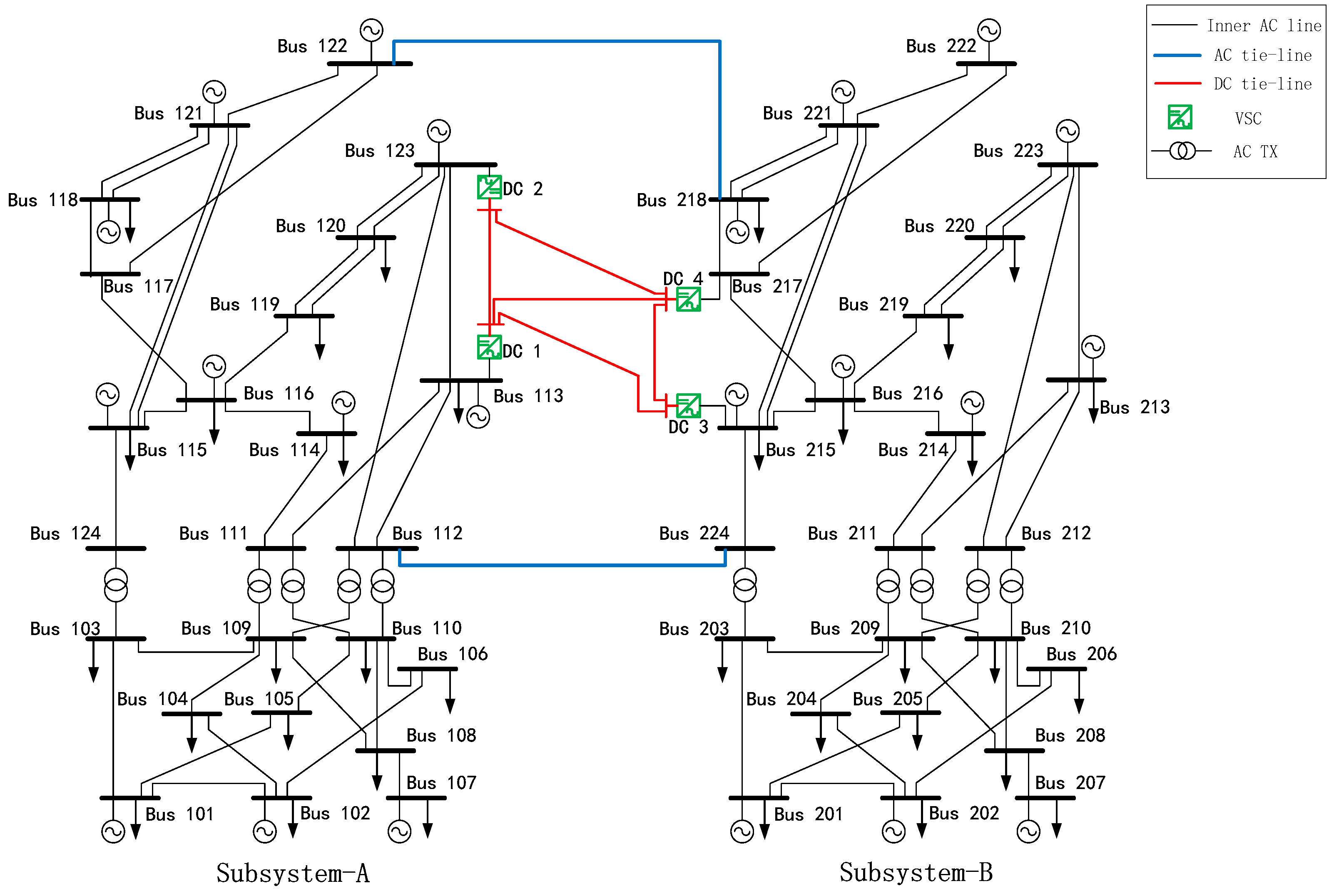
Figure 4 shows the modified single-line diagram of the MRTS network. On the basis of the original case data, the following modifications are made. In the 345 kV system, lines 113–215 and 123–217 are replaced by a 4-terminal 300 kV VSC-MTDC network, and two AC lines (122–218 and 112–224) are added as the AC tie-lines. In the 138 kV systems, line 107–203 is deleted. As shown in Figure 4, the entire test system is divided into two subsystems, namely, subsystems-A and -B. Bus 115 is regarded as the slack bus of the interconnected systems, and bus 214 is the active power balanced bus in subsystem-B.c. The AC tie-lines 122–218 and 112–224 and the four-terminal VSC-MTDC network form the transmission interface between subsystems. The BPTC is assumed as follows. A 360 MW active power is required to transfer from subsystem-A to subsystem-B directionally via the transmission interface. According to the voltage level, the maximum active power transmitted via a single AC tie-line should be no more than the upper limit of 240 MW.

Table 1. Impedance information of AC tie-lines.

Line	Resistance (p.u.)	Reactance (p.u.)	Susceptance (p.u.)
122–218	0.0490	0.3675	0.7735
112–224	0.0140	0.1050	0.2210

shows the impedance information of AC tie-lines.

Table 2. Basic parameters, initial controlling modes and setting values of VSCs.

Converter	1	2	3	4
Control Mode	$V_d$/$Q_s$	$P_s$/$Q_s$	$P_s$/$Q_s$	$P_s$/$Q_s$
$X_{\mathit{li}}$ (p.u.)	0.1121	0.1121	0.1121	0.1121
$R_i$ (p.u.)	0.0015	0.0015	0.0015	0.0015
$V_d$ (p.u.)	2.0	-	-	-
$V_{\mathit{ti}}$ (p.u.)	-	-	-	-
$Q_s$ (MVar)	18.62	6.19	−26.21	−22.96

VSC: voltage source converter.

presents the basic parameters, initial controlling modes, and the setting values of VSCs.

The sensitivity of active power transmitted via tie-lines to the active power output of generators $K_g^l$ can be calculated with (16)–(17). The sorted result is shown in

Table 3. Calculation result of sensitivity.

Gen No.	${\mathit{K}}_{\mathit{g}}^{\mathit{l}}$	Gen No.	${\mathit{K}}_{\mathit{g}}^{\mathit{l}}$
122	−0.1743	123	0.0467
107	0.0766	218	0.0324
102	0.0726	221	0.0218
101	0.0718	222	0.0218
114	0.0718	115	−0.0172

.

In Table 3, sensitivity $K_g^l$ indicates that when the active power output of the generator increases by 1 MW, the active power transmitted via tie-line 112–224 will increase $K_g^l$ MW and that transmitted via tie-line 122–218 will decrease $K_g^l$ MW accordingly. The sensitivity result shows that the generator at bus 122 is the DIPA unit, which has a deep influence on the power allocation. When the switching strategy of VSC controlling modes is adopted, the $V_{\mathit{tcr}}$ is set to 0.85 (p.u.).

5.2. The Influence of BPTC on VSM

The influence of BPTC on the VSM in the CPF calculation can be illustrated by comparing the simulation schemes M1 and M2. The control information of M1 and M2 are detailed as follows:

Scheme M1: The proposed CPF model in this study is applied. The nonlinear constraint equations of DTAP derived from the BPTC are considered. The security control behaviors for power allocation of tie-lines and the switch strategy of VSC controlling modes are also simulated in this scheme.

Scheme M2: All subsystems are simulated independently while ignoring the BPTC. The AC or DC tie-lines are assumed to be equivalent to the constant loads at the boundary buses of subsystems, and the equivalent loads can be calculated by the initial power flow. The controlling modes of VSCs are remained constant during load growth.

In the CPF, the critical load growth factor ${\lambda }_{\mathit{max}}$, which refers to the ratio of maximum additional load increment to the initial load, is commonly used to characterize the VSM. The ${\lambda }_{\mathit{max}}$ and the maximum active power transmitted in AC tie-lines under different schemes are shown in

Table 4. Maximum load growth factor and maximum active power transmitted in AC tie-lines.

Scheme	${\mathsf{\lambda }}_{\mathit{max}}$	Maximum Active Power Transmitted (MW)
M1	1.3102	235.03
M2	1.0857	163.09
M3	1.1744	294.76
M4	1.1907	257.92
M5	1.1179	227.15

. Schemes M3, M4, and M5 are the comparative schemes used in the latter part of this study, and their control information will be discussed in detail.

The ${\lambda }_{\mathit{max}}$ in Table 4 indicates that the critical load growth factor in scheme M1 is 1.3102, whereas that of scheme M2 is 1.0857, wherein the former is 1.21 times the latter. Hence, the VSM result will deviate far from the reality when the CPF model based on PQ equivalent method is applied.

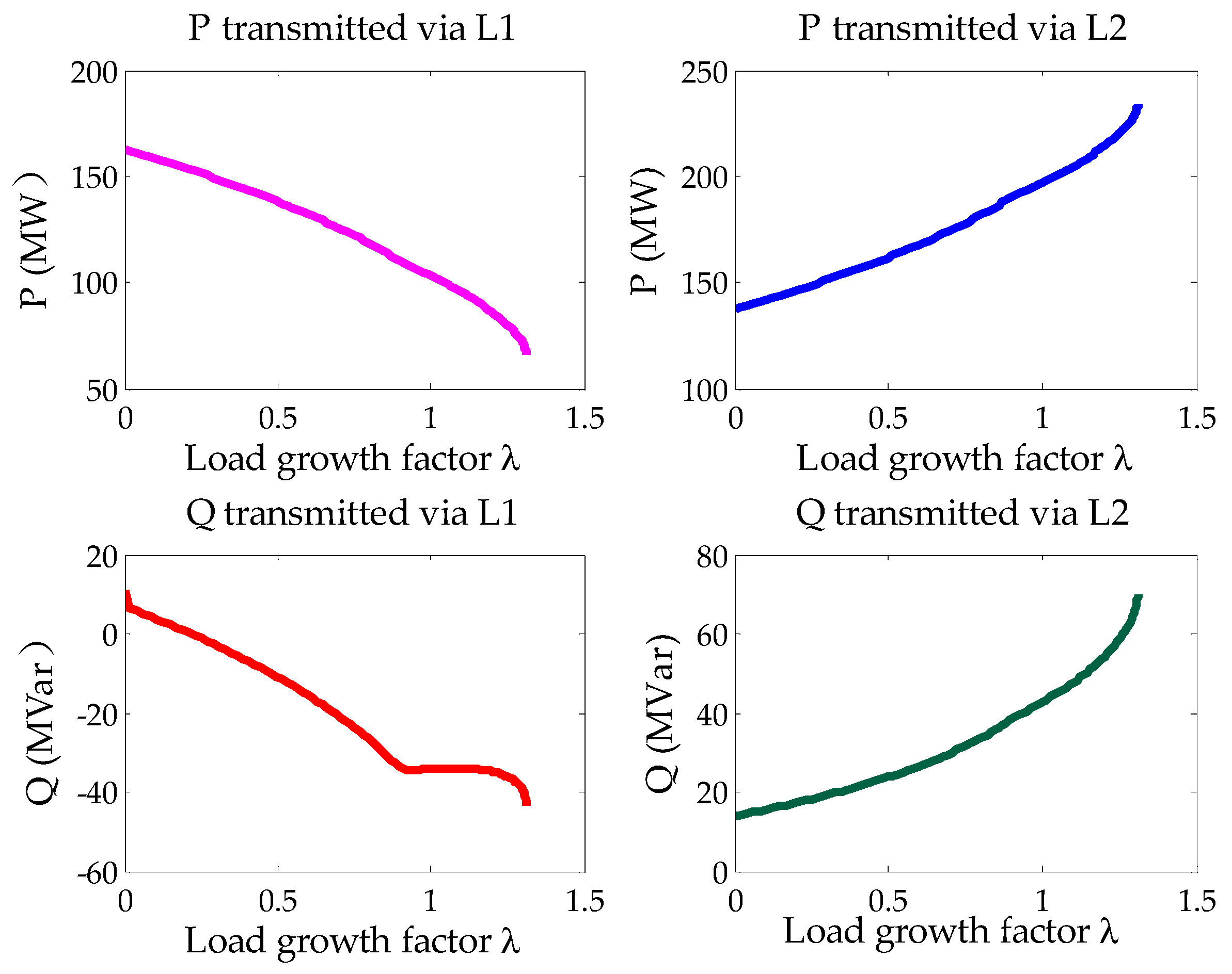
Figure 5 shows the curves of transmission power in AC tie-line L1 and L2 under scheme M1. L1 refers to line 112–224, whereas L2 refers to line 122–218. If the value of power is positive, then the power direction is from bus 112 to bus 224 or bus 122 to bus 218. As shown in Figure 5, with the load growth, the active power transmitted in L1 will decrease from 163.09 MW to 65.90 MW, and the reactive power transmitted in L1 will reverse from 10.86 MVar to −43.35 MVar. Apparently, with the introduction of BPTC, the power allocation proportion of tie-lines will have a dramatic change. Thus, the VSM under scheme M1 distinctly differs from that under scheme M2.

5.3. The Influence of the Selection Strategy for AGC Units

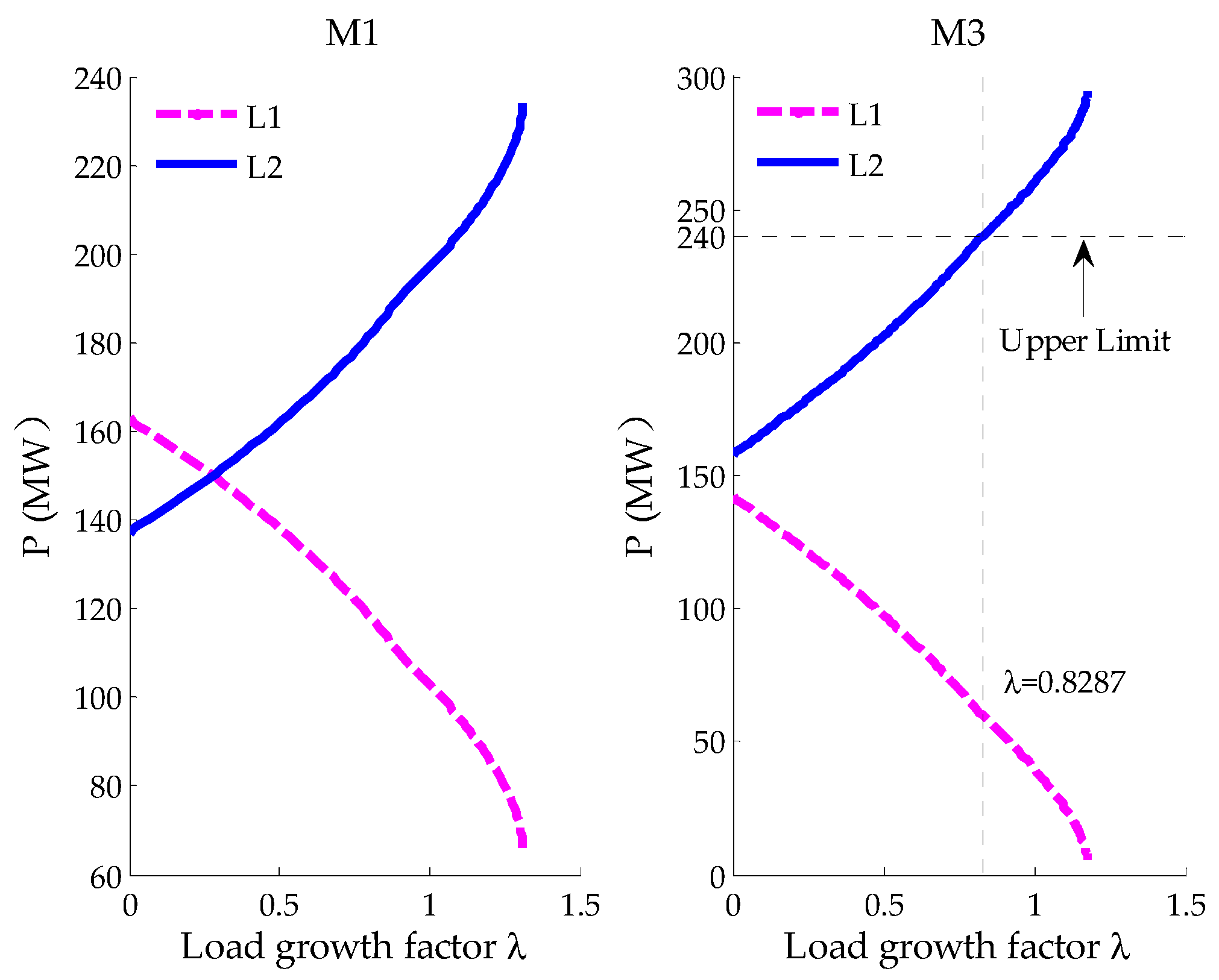
The influence of the proposed selection strategy for AGC units on the VSM and the power transfer security of tie-lines can be illustrated by comparing schemes M1 and M3. Scheme M1 has been previously described, and the control information of M3 is detailed as follows:

Scheme M3: This scheme is identical to scheme M1 in other aspects except for not simulating the selection strategy for AGC units, namely, Strategy-S1. Concretely, the DIPA unit (the generator at bus 122) is selected as an AGC unit. When the multi-balanced strategy is utilized to simulate the controlling behaviors of AGC units, bus 122 is also set as the slack bus.

Figure 6 shows the curves of transmission active power in AC tie-lines under schemes M1 and M3.

As shown in Figure 6, the difference of active power transmitted in tie-lines L1 and L2 initially decrease and then increase later under scheme M1. Furthermore, the maximum active power transmitted in tie-lines does not exceed the security upper limit 240 MW. On the contrary, under scheme M3, the difference of active power transmitted in tie-lines increases continuously. When λ reaches 0.8287, the active power transmitted in line L2 breaks through the security upper limit of 240 MW and continuously increase with the load growth. Therefore, in comparison with scheme M3, the active power allocation of tie-lines under scheme M1 is more balanced, and the requirement of security control for transmission active power in AC tie-lines is satisfied. Table 4 shows that the ${\lambda }_{\mathit{max}}$ under scheme M1 is 1.3102, and that under scheme M3 is 1.1744, wherein the former is 1.12 times of the latter.

The above simulation results indicate the following analysis. In addition to load increment, the AGC units also balance the active power loss of the entire interconnected systems. If the DIPA units are selected as the AGC units, the active power outputs of these units will increase rapidly during load growth. Then, the power allocation of tie-lines will change considerably, and the transmission active power in several tie-lines will exceed the security upper limit. In this situation, the VSM of the interconnected systems will decrease.

5.4. The Influence of the Generation Re-Dispatch Strategy on VSM

The influence of the proposed generation re-dispatch strategy on the VSM and the power transfer security of tie-lines can be illustrated by comparing schemes M1 and M4. Scheme M1 has been previously described, and the control information of M4 is detailed as follows:

Scheme M4: This scheme is identical to scheme M1 in other aspects except for not simulating the generation re-dispatch strategy, namely, Strategy-S2. In other words, the DIPA unit can participate in the distribution of load increment.

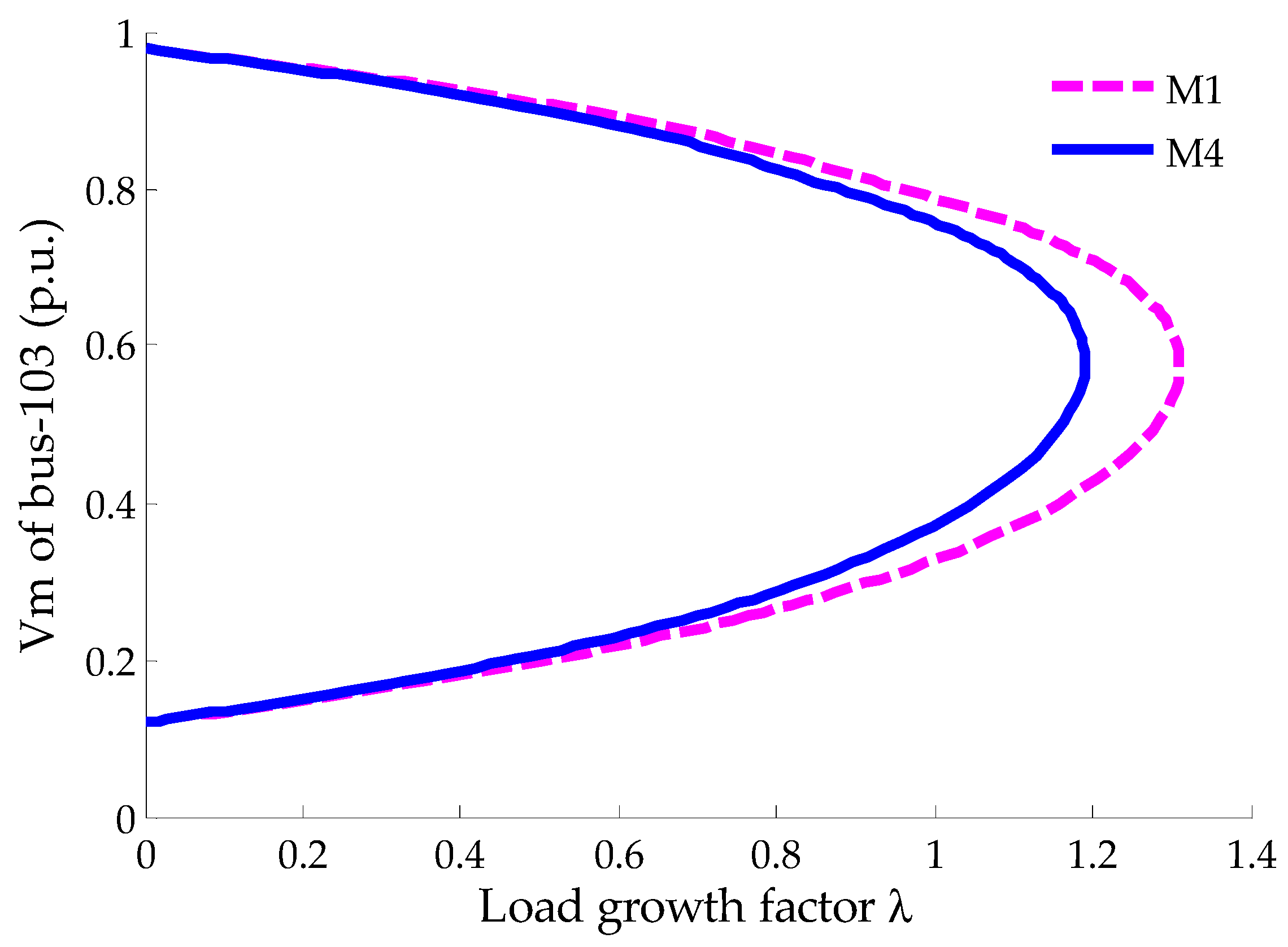
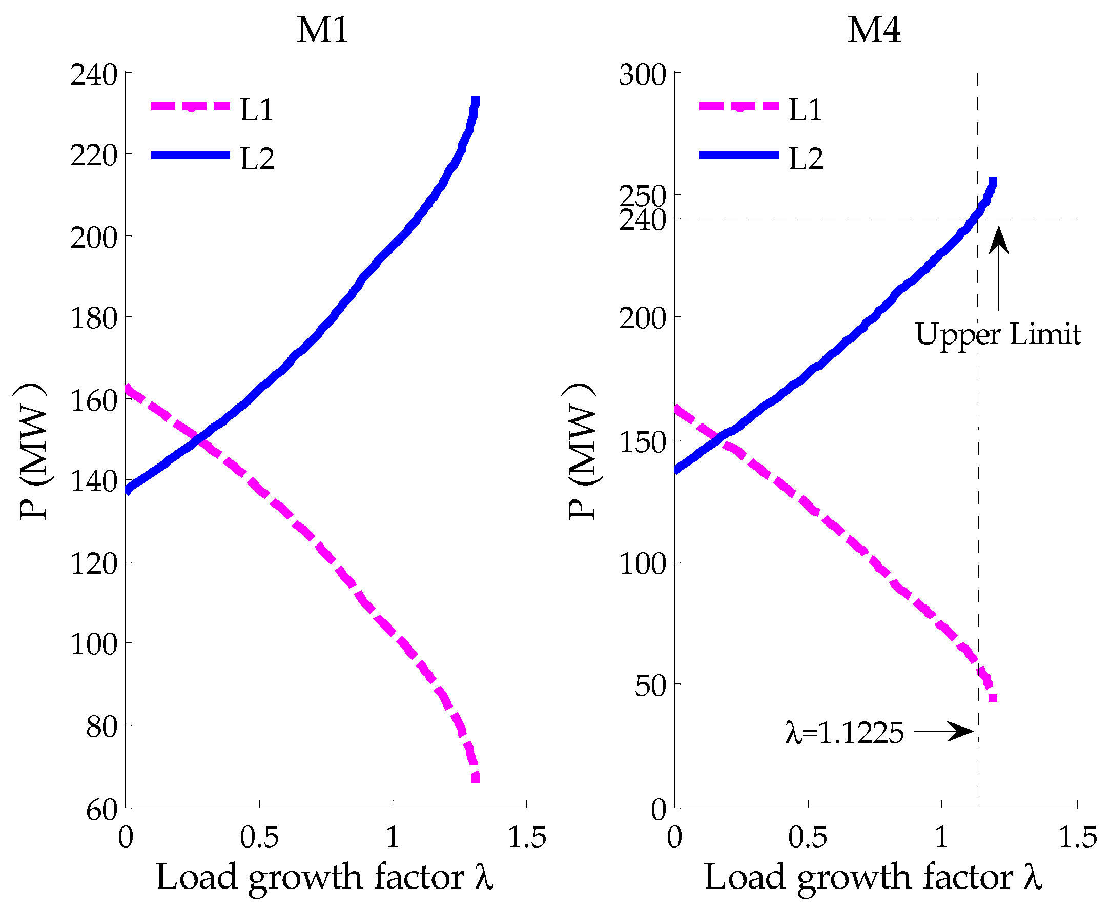
Figure 7 shows the V–$\lambda$ curves of typical buses (e.g., bus 103) under schemes M1 and M4, and the Figure 8 shows the curves of transmission active power in AC tie-lines under schemes M1 and M4.

The V–$\lambda$ curves in Figure 7 show that the critical load growth factor of scheme M1 is larger than that of scheme M4. As shown in Table 4, the ${\lambda }_{ma\mathit{x}}$ under scheme M1 is 1.3102 and that under scheme M4 is 1.1907. These results demonstrate that the VSM of the interconnected systems will be improved when the Strategy-S2 is applied. In comparison with scheme M1, the active power allocation of AC tie-lines under scheme M4 is relatively more concentrated (Figure 8). When $\lambda$ reaches 1.1225, the transmission active power in L2 exceeds the security upper limit of 240 MW under scheme M4. Thus, the VSM of scheme M4 is lower than that of scheme M1.

5.5. The Influence of Simulating the Switching Strategy for Reactive Power Control of VSC Stations

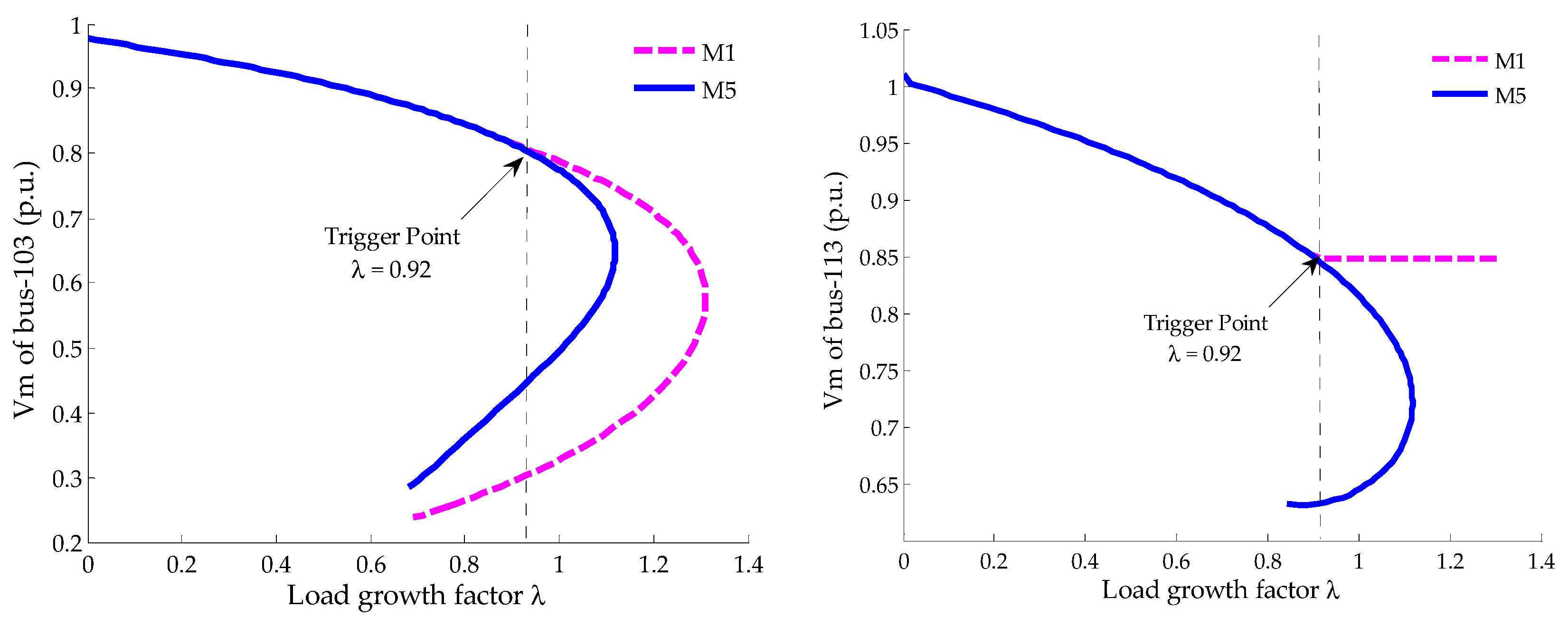
The influence of the proposed switching strategy for VSC controlling modes on the VSM can be illustrated by comparing scheme M1 and M5. Scheme M1 has been previously described, and the control information of M5 is detailed as follows:

Scheme M5: On the basis of scheme M1, the switching strategy of VSC controlling modes is not simulated.

Figure 9 shows the V–$\lambda$ curves under schemes M1 and M5, where bus 103 represents the common voltage weak buses and bus 113 refers to the PCC bus.

Under scheme M1, when $\lambda$ reaches 0.92, the voltage magnitude of bus 113 is below the threshold value $V_{\mathit{tcr}}$ 0.85. Then, the switching strategy of VSC controlling modes is activated. The controlling mode of VSC 1 switches from Mode 1) to Mode 2), and the voltage magnitude of bus 113 is prevented from continuing to decrease. The PCC buses are the key buses in the AC/DC interconnected systems. The VSM of the entire system can be improved when the voltage stability of PCC buses is guaranteed. As shown in Figure 9, even the common voltage weak buses can bear more load increment under Scheme M1. The simulation results in Table 4 imply that the critical load growth factor of scheme M1 is 1.3102 and that of Scheme M5 is 1.1179. Therefore, the VSM of interconnected systems is improved by 17.2% after adopting the switching strategy of VSC controlling modes.

5.6. Comparisons and Analysis of the Proposed Decoupling CPF Algorithm and the Integrated Algorithms

The computational accuracy and calculation speed of the proposed decoupling CPF algorithm can be illustrated by comparing with the integrated CPF algorithms in [17] and [21]. Reference [21] firstly proposed the CPF algorithm for AC systems, and all subsequent studies about CPF were its expansions and improvements. As one comparison, the prediction-correction calculation process of this algorithm will be applied to solve the CPF model for M-AC/VSC-MTDC interconnected systems in a centralized way. Reference [17] proposed a CPF algorithm for a hybrid AC/DC system with two-terminal VSC-HVDC, the main calculation of which is composed of an integrated prediction calculation and a distributed power flow calculation. As the other comparison, this algorithm will be extended to multi-terminal DC network. For the fairness of the result comparison, the arc-length parameterization will be adopted in all these three algorithms. To express these three algorithms conveniently, the proposed decoupling CPF algorithm, the integrated CPF algorithm in [17] and the integrated CPF algorithm in [21] are defined as DCA, ICA−I and ICA−II, respectively.

Table 5. Comparisons of proposed decoupling CPF algorithm and integrated algorithms under M1.

	DCA	ICA−I	ICA−II
Critical load growth factor ${\lambda }_{\mathit{max}}$	1.3102	1.3163	1.3085
Steps of prediction-correction	99	99	99
Numbers of iterations	417	752	417
Total calculation time (s)	4.8562	6.4755	7.5068

shows the calculated critical load growth factor ${\lambda }_{\mathit{max}}$, the steps of prediction-correction, the numbers of iterations and the total calculation time of the proposed decoupling algorithm and the integrated algorithms under Scheme M1.

Firstly, the computational accuracy of these three algorithms is compared and analyzed. By observing the simulation results in Table 5, the ${\lambda }_{\mathit{max}}$ calculated by these three CPF algorithms are very close, which all are around 1.31. Furthermore, the steps of prediction-correction required to increase initial load to the maximum in these three algorithms are the same. These results demonstrate that the proposed decoupling CPF algorithm has very high computational accuracy, and it is highly consistent with the integrated algorithms not only in the ultimate result, but also in the intermediate process. Theoretically, the forward and backward equations derived in the proposed decoupling algorithm are based on the strictly equivalent linear transformation, therefore its calculation accuracy is completely equivalent to the integrated calculation.

Then the calculation speeds of these three algorithms are compared and discussed. The total calculation time of the proposed decoupling CPF algorithm, ICA−I and ICA−II are 4.8562, 6.4755 and 7.5068 seconds, respectively. In addition, the numbers of iterations of these three algorithms are 417, 752 and 417, respectively. Obviously, the proposed decoupling CPF algorithm has an apparent advantage on the calculation speed by comparing with the other two integrated algorithms. With the bi-directional iteration, the proposed decoupling CPF algorithm simplifies the hybrid AC/DC prediction equation and correction equation, eliminates 6/7 DC variables and only retains the variable $V_{\mathit{ti}}$. This algorithm reduces the dimensions of calculation equations in each prediction-correction step and improves the calculation speed.

6. Conclusions

This study proposes a novel CPF model for M-AC/VSC-MTDC. The BPTC among subsystems, the security control behaviors for power allocation of tie-lines, and switching characteristic of reactive power control behaviors of VSC stations are considered in the proposed model. Furthermore, a novel decoupling CPF algorithm based on bi-directional iteration is also presented to realize the decomposition and coordination calculation. Case studies and comparative analysis on the IEEE two-area RTS-96 system indicate the effectiveness and validity of the proposed CPF model and decoupling algorithm. The following conclusions can be drawn:

(1)

The BPTC has a great influence on the CPF calculation for interconnected systems. Ignoring this influence will render the calculated VSM deviate far from reality. The derived nonlinear constraint equations of DTAP and the multi-balancing machine strategy have been proven effective in simulating the influence of BPTC on CPF calculation.

(2)

In the case studies, the simulation result shows that the power allocation proportion of tie-lines will change considerably during load growth. In extreme situations, serious overload in tie-lines may occur. The proposed selection strategy for AGC units and the generation re-dispatch strategy can work together to prevent the overload in tie-lines and improve the VSM.

(3)

The switching characteristic of reactive power control behaviors of VSC stations is simulated in the CPF model. The simulation shows that the VSM of the M-AC/VSC-MTDC interconnected systems will improve remarkably when the switching strategy is adopted.

(4)

The simulation result demonstrates that the proposed decoupling CPF algorithm has very high computational accuracy, and it is highly consistent with the integrated algorithms not only in the ultimate result, but also in the intermediate process. At the same time, the simulation comparison also shows the proposed decoupling CPF algorithm has an apparent advantage on the calculation speed by comparing with the integrated algorithms.

References

1. Adusumilli, B.S.; Kumar, B.K. Modified affine arithmetic based continuation power flow analysis for voltage stability assessment under uncertainty. IET Gener. Transm. Distrib. 2018, 12, 4225–4232. [Google Scholar] [CrossRef]
2. Zhao, J.; Wang, Y.; Xu, P. A comprehensive on-line voltage stability assessment method based on continuation power flow. In Proceedings of the 2009 International Conference on Sustainable Power Generation and Supply (SUPERGEN), Nanjing, China, 6–7 April 2009; pp. 1–5. [Google Scholar]
3. Barnes, M.; Hertem, D.V.; Teeuwsen, S.P.; Callavik, M. HVDC systems in smart grid. Proc. IEEE 2017, 105, 2082–2098. [Google Scholar] [CrossRef]
4. Wang, H.C.; Pietro, G.D.; Wu, X.Z.; Lahdelma, R.; Verda, V.; Haavisto, I. Renewable and sustainable energy transitions for countries with different climates and renewable energy sources potentials. Energies 2018, 11, 3523. [Google Scholar] [CrossRef]
5. Li, X.L.; Yuan, Z.C.; Fu, J. Nanao multi-terminal VSC-HVDC project for integrating large-scale wind generation. In Proceedings of the 2014 IEEE PES General Meeting/Conference & Exposition, National Harbor, MD, USA, 30–31 October 2014; pp. 1–5. [Google Scholar]
6. Hierarchical Control in a 5-Terminal VSC-HVDC Project. 2014. Available online: http://www.ee.co.za/article/hierarchical-control-5-terminal-vsc-hvdc-project.html (accessed on 11 November 2014).
7. Zhang, X.P. Multiterminal voltage-sourced converter-based HVDC models for power flow analysis. IEEE Trans. Power Syst. 2004, 19, 1877–1884. [Google Scholar] [CrossRef]
8. Beerten, J.; Cole, S.; Belmans, R. Generalized steady-state VSC MTDC model for sequential AC/DC power flow algorithms. IEEE Trans. Power Syst. 2012, 27, 821–829. [Google Scholar] [CrossRef]
9. Chai, R.Z.; Zhang, B.H.; Dou, J.M.; Hao, Z.G.; Zheng, T. Unified power flow algorithm based on the NR method for hybrid AC/DC grids incorporating VSCs. IEEE Trans. Power Syst. 2016, 31, 4310–4318. [Google Scholar] [CrossRef]
10. Khan, S.; Bhowmick, S. A generalized power flow model of VSC based hybrid AC-DC systems integrated with offshore wind farms. IEEE Trans. Sustain. Energy 2018. early access. [Google Scholar] [CrossRef]
11. Chaudhuri, N.R.; Majumder, R.; Chaudhuri, B.; Pan, J.P. Stability analysis of VSC MTDC grids connected to multimachine AC systems. IEEE Trans. Power Deliv. 2011, 26, 2774–2784. [Google Scholar] [CrossRef]
12. Beerten, J.; Cole, S.; Belmans, R. Modeling of multi-terminal VSC HVDC systems with distributed DC voltage control. IEEE Trans. Power Syst. 2014, 29, 34–42. [Google Scholar] [CrossRef]
13. Khan, S.; Bhowmick, S. A comprehensive power flow model of multi-terminal PWM based VSC-HVDC systems with DC voltage droop control. Int. J. Elec. Power Energy Syst. 2018, 102, 71–83. [Google Scholar] [CrossRef]
14. Chen, H.R.; Wang, C.; Zhang, F.; Pan, W.L. Control strategy research of VSC based multi-terminal HVDC system. In Proceedings of the 2006 IEEE PES Power Systems Conference and Exposition, Atlanta, GA, USA, 29–31 October 2006; pp. 1986–1990. [Google Scholar]
15. Li, Z.; He, Y.; Li, Y.Z.; Gu, W.; Tang, Y.; Zhang, X.P. Hybrid control strategy for AC voltage stabilization in bipolar VSC-MTDC. IEEE Trans. Power Syst. 2019, 34, 129–139. [Google Scholar] [CrossRef]
16. Liang, J.; Gomis-Bellmunt, O.; Ekanayake, J.; Jenkins, N. Control of multi-terminal VSC-HVDC transmission for offshore wind power. In Proceedings of the 2009 13th European Conference on Power Electronics and Applications, Barcelona, Spain, 8–10 September 2009. [Google Scholar]
17. Wang, Z.H.; You, Z.Y.; Huang, Y.L. load margin analysis of hybrid AC/DC system with two terminal VSC-HVDC using continuous power flow method. Power Syst. Prot. Control 2018, 46, 9–15. (In Chinese) [Google Scholar]
18. Chen, H.H.; Huang, Y.L.; Jiang, T.; Li, X.; Li, G.Q. Voltage stability analysis and control for AC/DC system with VSC-HVDC. Power Syst. Technol. 2017, 41, 2429–2435. [Google Scholar]
19. Gao, Y.J.; Wang, Z.; Liang, H.F. Available transfer capability calculation with large offshore wind farms connected by VSC-HVDC. In Proceedings of the 2012 IEEE PES Innovative Smart Grid Tech., Tianjin, China, 21–24 May 2012; pp. 1–6. [Google Scholar]
20. Iba, K.; Suzuki, H.; Egawa, M. Calculation of critical loading condition with nose curve using homotopy continuation method. IEEE Trans. Power. Syst. 1991, 6, 584–593. [Google Scholar] [CrossRef]
21. Ajjarupu, V.; Christy, C. A tool for steady state voltage stability analysis. IEEE Trans. Power Syst. 1992, 7, 416–423. [Google Scholar] [CrossRef]
22. Alves, D.A.; Da Silva, L.C.P.; Castro, C.A. Continuation fast decoupled power flow with secant predictor. IEEE Trans. Power Syst. 2003, 18, 1078–1085. [Google Scholar] [CrossRef]
23. Flueck, A.J.; Dondeti, J.R. A new continuation power flow tool for investigating the nonlinear effects of transmission branch parameter variations. IEEE Trans. Power Syst. 2000, 15, 223–227. [Google Scholar] [CrossRef]
24. Dong, X.M.; Wang, C.F.; Liang, J. Calculation of power transfer limit considering electro-thermal coupling of overhead transmission line. IEEE Trans. Power Syst. 2014, 29, 1503–1511. [Google Scholar] [CrossRef]
25. Li, S.H.; Chiang, H.D. Continuation power flow with nonlinear power injection variations: A piecewise linear approximation. IEEE Trans. Power Syst. 2008, 23, 1637–1643. [Google Scholar] [CrossRef]
26. Lei, J.T.; An, T.; Du, Z.C. A general unified AC/DC power flow algorithm with MTDC. IEEE Trans. Power Syst. 2017, 32, 2837–2846. [Google Scholar] [CrossRef]
27. Beerten, J.; Hertem, D.V.; Belmans, R. VSC-MTDC systems with a distributed DC voltage control—A power flow approach. In Proceedings of the IEEE Power Tech’11, Trondheim, Norway, 19–23 June 2011. [Google Scholar]
28. Guo, H.Y.; Liu, M.B.; Lin, S.J. Analysis of effect of secondary voltage control on static stability. Autom. Electr. Power Syst. 2011, 35, 20–24. [Google Scholar]
29. Zheng, C.; Zhou, X.X.; Li, R.M.; Sheng, C.H. Study on the steady characteristic and algorithm of power flow for VSC-HVDC. Proc. CSEE 2005, 25, 1–5. [Google Scholar]
30. Wang, W.; Barnes, M. Power flow algorithms for multi-terminal VSC-HVDC with droop control. IEEE Trans. Power Syst. 2014, 29, 1721–1730. [Google Scholar] [CrossRef]
31. Chiang, H.D.; Flueck, A.J. A practical tool for tracing power system steady-state stationary behavior due to load and generation variations. IEEE Trans. Power Syst. 1995, 10, 623–634. [Google Scholar] [CrossRef]
32. Canizares, C.A.; Alvarado, F.L. Point of collapse and continuation methods for large AC/DC systems. IEEE Trans. Power Syst. 1993, 8, 1–8. [Google Scholar] [CrossRef] [Green Version]
33. Zhao, J.; Chiang, H.D.; Li, H. A new contingency parameterization CPF model and sensitivity method for voltage stability control. In Proceedings of the IEEE PES General Meeting 2005, San Francisco, CA, USA, 4–6 July 2005; pp. 1–7. [Google Scholar]
34. Reliability Test System Task Force. The IEEE reliability test system-1996: A report prepared by the reliability test system task force of the application of probability methods subcommittee. IEEE Trans. Power Syst. 1999, 14, 1010–1020. [Google Scholar] [CrossRef]
Figure 1. Steady-state physical model of VSC-MTDC network. VSC: voltage source converter; MTDC: multi-terminal direct current.
Energies 12 00733 g001
Figure 2. Schematic of multi-area interconnected system.
Energies 12 00733 g002
Figure 3. Calculation flow chart of CPF for M-AC/VSC-MTDC interconnected systems.
Energies 12 00733 g003
Figure 4. MRTS system with a 4-terminal VSC-MTDC network.
Energies 12 00733 g004
Figure 5. Curves of transmission power in AC tie-lines under scheme M1.
Energies 12 00733 g005
Figure 6. Curves of active power transmitted in tie-lines under schemes M1 and M3.
Energies 12 00733 g006
Figure 7. V–λ curves of typical buses under schemes M1 and M4.
Energies 12 00733 g007
Figure 8. Curves of active power transmitted in tie-lines under schemes M1 and M4.
Energies 12 00733 g008
Figure 9. The V–λ curves under schemes M1 and M5.
Energies 12 00733 g009