Abstract
In this study we evaluated the wind resources of wind farms in the Changhua offshore area of Taiwan. The offshore wind farm in Zone of Potential (ZoP) 26 was optimized through an economic evaluation. The annual energy production (AEP) of the offshore wind farm in ZoP 26 was predicted for 10 and 25 years with probabilities of 50%, 75%, and 90% by using measured mast data, measure-correlate-predict (MCP) data derived from Modern-Era Retrospective Analysis for Research and Applications (MERRA), and Central Weather Bureau (CWB) data. When the distance between the turbines in a wind farm was decreased from 12D to 6D, the turbine number increased from 53 to 132, while the capacity factor decreased slightly from 48.6% to 47.6%. MCP data derived from the inland CWB station with similar levels of wind resources can be used to accurately predict the power generation of the target offshore wind farm. The use of MCP with mast data as target data, together with CWB and MERRA data as reference data, proved to be a feasible method for predicting offshore wind power generation in places where a mast is available in a neighboring area.
1. Introduction
Offshore wind energy is regarded as the backbone that can replace domestic nuclear energy and fossil fuels according to national energy policy of Taiwan. This policy is justified by the fact that the Taiwan Strait has excellent potential for wind energy generation. According to 4C Offshore, 25 projects exist with a 10-year mean wind speed higher than 12 m/s for a hub height of 100 m, and most such projects are located in the Taiwan Strait [1].
Over the past 20 years, a number of methodologies have been developed to evaluate offshore wind resources. Because of the difficulty of measurement campaigns in offshore areas, the measured wind data for a targeted wind farm often cover only 1 year or even a shorter time. Such limited data sets cannot characterize long-term wind resources. An alternative approach known as measure, correlate, predict (MCP) has been developed to sample long-term wind data at the site of a targeted wind farm. MCP is typically used to relate and adjust on-site measurements to a set of long-term reference data. This process has been widely used in wind energy research [2], and has become crucial for evaluating regional wind potential at sites that lack local long-term wind data.
The Weibull distribution is widely used as a basis for wind resource evaluation. It is a mathematical function that can represent the wind speed frequency distribution at a site. In the Weibull distribution, the probability density (frequency distribution) represents the number of times in the period of record that the observed speed falls within particular ranges [3]. The speed bins are typically 0.5 or 1 m/s wide and span at least the range of speeds defined for the turbine power curve from 0 to 25 m/s and above. It is usually presented in reports as a bar chart covering all directions. A study examined the accuracy of Weibull distribution using observation data from three weather stations on three islands near Hong Kong over a period of six years. The result indicated that Weibull distribution had accurately represented the real offshore wind speed frequency [4].
The capacity factor is often used to assess wind resources at a given site. It is the energy delivered during a period of time expressed as a fraction of the energy that would have been supplied if the plant had operated at its rated capacity. The annual capacity factor is the energy generated during the year (MWh) divided by wind farm rated power (MW) multiplied by the number of hours in the year [5]. Capacity factors are also affected by the efficiency of the turbine and its suitability for its particular location [6]. High capacity factors indicate efficient utilization of the generator. The capacity factor is affected by the wind conditions and the turbine’s swept area. A small turbine usually generates relatively low power for high wind speed because of the short length of its blades. Conversely, a large turbine generates more power for a high speed but its cut-in speed is larger than that of a small turbine. With advances in technology, the capacity factor of Anholt 1 offshore wind farm in Denmark reached 52.8%. The average capacity factor of offshore wind farms in Denmark is 41.9% [7].
For the optimization of offshore wind farm layout, proposed optimization schemes generally prioritize costs [8]. A study proposed a method of evaluating the net present value of all costs, including initial, construction, operation and maintenance, and retirement costs, and the revenue from selling the produced energy on a life-cycle basis; the Weibull distribution, wind rose, and energy production loss caused by wake loss effects were included in that assessment [9].
Currently, typical wind resource evaluations are mainly based on historical weather observations, numerical simulation, satellite-based remote sensing, and reanalysis of data [10]. Historical observations refer to using instruments to measure wind speed and wind direction to characterize the wind resources of a specific site. A problem with this type of evaluation is the limited observation range. Pimenta et al. [11] used both weather observation data and satellite data sets to evaluate the location, seasonal timing, and availability of wind power resources for the southern coast of Brazil. Meteorological stations measure directly at a high time resolution but low spatial resolution and allow for validation and adjustment of satellite data, whereas satellite data provide near-complete spatial coverage at a lower time resolution.
To overcome the costs and inconveniences of surface-based wind monitoring systems, software-based numerical simulations of microscale wind resources have been developed. Some widely used simulation tools are WAsP, MM5, MesoMap, Site Wind, TAPM, and WEST [10]. Researchers mostly apply integrated model systems to evaluate wind energy resources; such systems are composed of a mesoscale meteorological numerical model, usually the Weather Research and Forecasting (WRF) model or MM5, and a complex-terrain dynamic diagnosis model, usually the California Meteorological Model or Advanced Regional Prediction System [12]. Salvação and Soares [13] used the WRF model to evaluate the offshore wind resources on the Iberian Atlantic coast. A 10-year wind hindcast was simulated with the WRF model at 9 and 3 km of spatial resolution and 6-hourly output. These simulation tools can evaluate wind resources rapidly and economically. However, the selection of boundary conditions and parameters can lead to inaccurate conclusions that bear little resemblance to real situations. Over the past 20 years, software for evaluating wind energy has improved enormously; such software now offers computational fluid dynamics (CFD), finite element analysis, and numerical modeling. Such simulations involve wind farm siting, wind farm modeling, prediction, and other items [14].
Satellite-based remote sensing systems have been developed to gather information about the Earth. This type of measurement can monitor the Earth on a long-term and large-scale basis without being restricted by terrain. During 2004–2006, the Risø National Laboratory in Denmark and several other research institutions conducted the SAT-WIND research program and confirmed the potential of applying satellite-derived data, including surface wind distribution data derived from passive microwave remote sensors, altimeters, scatterometers, and synthetic aperture radars (SARs), to offshore wind energy resource evaluation. The results showed that it was feasible to evaluate offshore wind energy resources using satellite-derived wind speed distributions. Charlotte et al. [15] used ocean surface wind speed data derived from SARs to study wind energy resources over the Baltic Sea. They compared the wind speed data derived from SARs with observational surface wind speed data and found that the SARs exhibited higher accuracy. However, such measurements are limited by (1) low time resolution (e.g., 14 of 17 satellites in the Danish SAT-WIND project record observations less than once a day); (2) low horizontal resolution, with a general satellite data resolution of 25 km × 25 km, except for SARs achieving finer spatial resolution; (3) low accuracy (e.g., wind speeds estimated by QuikSCAT satellite-based remote sensing are overestimated with an average deviation of 1.00–3.63 m/s); (4) and few options for height of observations (wind flow at 10 m may be provided by satellites that cannot depict wind flows at different heights) [3,10].
Various reanalysis data sets have been developed to provide high quality, long time scales, and regular grid points. In the mid-1990s, the US National Center for Environmental Prediction (NCEP) collaborated with the National Center for Atmospheric Research (NCAR) to develop the first-generation reanalysis data product NCEP-R1 [16]. The European Center for Medium-range Weather Forecast (ECMWF) subsequently published its first-generation reanalysis data product, ERA-15. The NCEP and ECMWF launched their second- and third-generation reanalysis data products during the 2000s [17,18,19].
Reanalysis data sets are created using historical weather observations to drive a global or regional NWP model. From these model runs, weather parameters are extracted for every grid point and every level in the model. Reanalysis data sets are created to support climate studies. Through statistical analysis of 10-m NCEP/DOE Reanalysis wind data from 1979–2010, Chadee and Clarke [20] derived a regional annual wind resource map, which showed that the Caribbean low-level jet region was an area with superb wind power density. They also identified the eastern Caribbean and the Netherlands Antilles as locations with excellent wind energy resources.
Reanalysis data have a number of positive attributes, including convenience, multiple levels and types of weather parameters, and a long data record. Because the gridded data are available for everywhere covered by the model, it is easy to locate suitable grid points. This eliminates much work searching for surface weather stations and data sets, and it provides a common data source for all MCP studies. In parts of the world where surface weather observations are unreliable, reanalysis data may be the only feasible source of reference data for MCP. However, reanalysis data also have significant disadvantages and must be used with caution. First, the correlation of the reanalysis of winds with tower observations depends on the complexity of the terrain and the resolution of the reanalysis model. The NCEP/NCAR global reanalysis data set is relatively coarse, with a resolution of about 2° in latitude and longitude (slightly over 200 km) and thus may provide poor results in mountainous terrain, at coastal boundaries, and in other places where sharp wind gradients exist. More importantly, the homogeneity of reanalysis data is limited by that of the observational system used to drive the model; observational systems have changed dramatically over the decades. The bulk of the weather observations in the 1950s and 1960s came from weather balloons supplemented by land- and ship-based surface observations. Weather satellites became increasingly important in the 1970s and 1980s, decades that were marked also by a large increase in the frequency of weather observations from both surface and radiosonde stations [11].
Concerning the evaluation software of wind energy, the first WAsP developed has been widely used in wind energy research. Measured wind data were used on the Turkish west coast from 1975 to 1984 to estimate wind resources using WAsP [21]. Another study evaluated wind conditions in the Danish offshore area of the Baltic Sea using WAsP and two measurement stations on Lolland Island. The result indicated that the WAsP simulation roughly conformed to wind conditions, except that its prediction slightly overestimated wind speed [22]. A study combined ArcGIS with WAsP to estimate wind resource distribution using ArcGIS to overlay WAsP’s estimates of the average wind speed and power density on a map of the studied region to determine the most suitable sites for installing wind turbines [23].
To reduce the deviation of wind resource evaluation caused by complex terrain, researchers have used CFD for relatively accurate simulation. The most widely used CFD-based software products for wind farm design are Meteodyn WT and WindSim. A study used mesoscale wind data and Meteodyn WT to evaluate the wind conditions on Phaluay Island in Thailand with a spatial resolution of 90 m × 90 m. The result accurately conformed to the mesoscale wind data [24]. Another study used Meteodyn WT to evaluate a wind farm on complex terrain. The result indicated that the wind resource evaluation of Meteodyn WT roughly conformed to measured data, but the simulation of extreme wind speed was relatively conservative [25]. WindSim can solve nonlinear equations of mass, momentum and energy; thus, it can simulate places with complex terrain and complex local climatic conditions. Researchers built more than 120 terrain models from data of heights and roughness covering the Norwegian coast from southern Lindesnes to the northern boundary with Russia and subsequently used WindSim to evaluate wind resources on the Norwegian coast [26]. According to a number of scientific research studies and practical engineering experiments, CFD-based calculation software can simulate wind resources more accurately than WAsP [27,28,29].
The accuracy with which a wind farm’s power generation can be estimated and predicted deeply influences the financial evaluation of the wind farm under consideration. Until now, because of the inconvenience of wind measurement in offshore areas, wind companies have mostly used mast and LiDAR methods to gather wind data. However, in some offshore areas, it is difficult for a LiDAR installation to survive extreme weather conditions long enough to gather representative data for wind resource evaluation. Considering that the offshore Zone of Potential (ZoP) 26 wind farm of Taiwan will be exploited in the future, in the present study, we aim to evaluate wind resources and optimize the design of the ZoP 26 wind farm by using data from mast, Modern-Era Retrospective Analysis for Research and Applications (MERRA), and weather stations. First, the power generation potential of the ZoP 26 wind farm is estimated (Figure 1). Second, the number of turbines in the target wind farm is optimized based on economic analysis. Finally, the probability of prediction of annual energy production (AEP) is evaluated based on the estimated uncertainty.
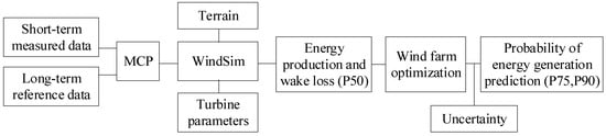
Figure 1.
Flowchart of this study.
2. Materials and Methods
2.1. Measurement Setup
The measurement locations considered in the present study are in the Changhua nearshore area of Taiwan (Figure 2). The Taipower mast is located 6 km from the coast. The height of the Taipower mast is 95 m above sea level, and the depth is 15 m below sea level (Figure 3). The height of the platform is 19 m above sea level. Three booms stretch out from the mast along the directions of 30°, 150°, and 270°. Considering the characteristics of wind resources in Taiwan with the northeast monsoon in winter and southwest airflow in summer, an anemometer and a wind vane are installed on the boom at 150°.
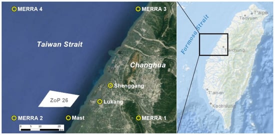
Figure 2.
Locations of wind farm in ZoP 26, Taipower meteorological mast, MERRA locations 1–4, and CWB stations at Lukang and Shenggang.
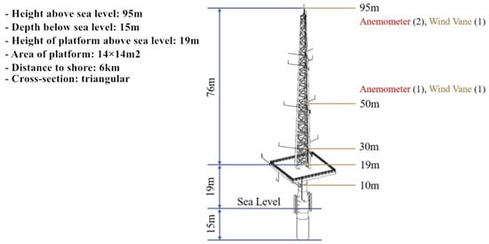
Figure 3.
Taipower offshore meteorological mast.
The cup anemometer and wind vane installed on the mast conform to the IEC 61400-12-1 Class 1. The permissible ambient temperature range for their operation is −50 °C to 80 °C. The anemometer can measure wind speeds of 0.3 m/s to 70 m/s with an accuracy of less than 0.2 m/s. The wind vane can measure angles of 0° to 360° with an accuracy of 1°.
The data measured by these instruments were collected with a data logger inside a container on the platform. The signal was transmitted by a microwave antenna on the mast. The receiver was installed on the roof of the Wanggong substation. The data were stored in a computer in the substation. A diesel generator was used to power the crane. Nine solar panels were used to supply power to the anemometer, wind vane, atmospheric pressure gauge, thermohygrometer, and data logger.
2.2. Datasets
The data sources used in this study are as follows: Taipower mast, MERRA, and Central Weather Bureau (CWB). Ideally, data sets should span at least 1 year of measurement, and cover an integer number of years to reflect the full seasonal cycle of wind variations. Hourly or 10-min wind speed and wind direction data are usually used. The Taipower mast started its measurement campaign on 1 April 2016; therefore, data from 1 April 2016 to 1 April 2017 were used in this study. MERRA and CWB Lukang data from 1 April 2011 to 1 April 2017, and CWB Shenggang data from 1 April 2012 to 1 April 2017 were used in this study. Although the Shenggang station began measurement in February 2011, it did not transmit data until 1 November 2011. The used data period thus starts from 2012 and contains a full year of data. Because the MERRA and CWB data have a resolution of no more than 1 h, hourly data from the Taipower mast, MERRA, and CWB were used in this study to ensure a consistent resolution for all data sources.
MERRA is an analysis method designed by NASA. The MERRA dataset spans the period from 1979 through 2016. The present study used data of MERRA version 2 (MERRA-2), which was started in 1980. MERRA and MERRA-2 are based on the GEOS-5 atmospheric data assimilation system, but additional advances to the GEOS model and the Gridpoint Statistical Interpolation assimilation system are included in MERRA-2. The MERRA data structures used in the present study are composed of four grid points (Figure 2). The MERRA data were simulated at a height of 50 m.
The Central Weather Bureau (CWB) data were obtained through the Central Observation Data Inquiry System (CODiS). The instrument used by CWB for measuring wind speed and wind direction is a propeller-type wind anemometer. The wind direction provided by CODiS is 0° when the wind speed is lower than 0.3 m/s. CODiS shows hourly wind speed data with an accuracy of one decimal place and shows the wind direction angle as an integer value. CODiS data from the Lukang and Shenggang stations, located at altitudes of 17 m and 24 m, respectively, were used in this study.
2.3. MCP
MCP is used to perform long-term hindcasting of wind resources at a target site with only short-term wind data. Various periods have been suggested for long-term data, such as three years [30], 10 years [31], and longer [32]. The long-term data series must coincide in the time series with the short-term data. Moreover, for such long-term data, the use of hourly data may be more suitable than the use of 10-min average wind data [33].
In the MCP method, the wind speed relationship between the target data and reference data would be reliable in the presence of a strong wind direction relationship between the target data and reference data. Correlation coefficient (R2) values in the ranges of 0.5–0.6, 0.6–0.7, 0.7–0.8, 0.8–0.9, and 0.9–1.0 are considered very poor, poor, moderate, good, and very good [34]. To express the characteristics of wind resources at the target site, data of at least a year should be used [35,36]. By using the relationship of coincident time period between the target data and reference data, unavailable target data can be synthesized from the reference data.
2.4. AEP
AEP is usually calculated as follows:
where is the number of hours in a year (=8760), and and are the Weibull distribution and the power output, respectively. The wake effect and the number of turbines must be considered when assessing the energy produced by a wind farm.
2.5. WindSim Model
WindSim is a wind farm design tool that can be used to build a numerical model of terrain by using elevation and roughness data. The code is based on the numerical core PHOENICS, which solves the Reynolds-Averaged Navier-Stokes (RANS) equation [37]. The equation can be used with approximations based on knowledge of the properties of flow turbulence to obtain approximate time-averaged solutions of the Navier–Stokes equation. The equation can be written as follows:
where represents the change in the mean momentum of the fluid element, represents mean body force, represents isotropic stress due to the mean pressure field, represents viscous stresses, and represents the Reynolds stress.
This equation is solved using computational fluid dynamics (CFD). Convergence of this equation with the Reynolds stress term is difficult, so a turbulence model is usually added. Before the CFD calculations, the domain is built based on the elevation and roughness of the target site.
In offshore areas, farm dynamics are mainly driven by wakes. WindSim is suitable for application to offshore test cases [38]. Compared to other software packages, WindSim has high consistency in terms of the topographic effect, and assessment results obtained using WindSim have been found to differ by 1% from real production data [39]. The rotor of a wind turbine is modeled as an actuator disc [40], which is applied to model the wakes of wind turbines in combination with RANS simulations [41].
In the simulation process of WindSim, terrain and wind data are imported. Thereafter, the boundary conditions and parameters of the turbine are set up.
2.5.1. Terrain Setup
In the present study, we employed ASTER GDEM v2 Worldwide Elevation Data with a resolution of 1 arc-second (approximately 30 m) to establish elevation data for the Changhua nearshore area. The roughness data were obtained from GlobeLand30 with a resolution of 30 m. The data contained in ASTER GDEM v2 Worldwide Elevation Data and GlobeLand30 were recorded using the WGS84 coordinate system. These two data sources were imported into the Global Mapper used to convert WGS84 into the UTM 51N coordinate system and combine the two data sources into a GWS file for import into WindSim. The elevation and roughness of terrain of the Changhua nearshore area are illustrated in Figure 4.
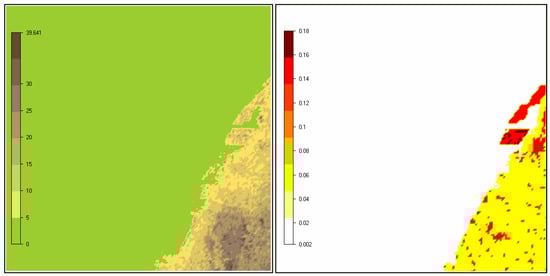
Figure 4.
Elevation (left) and roughness (right) of terrain of Changhua nearshore area.
To ensure that the AEP calculation converged, the mesh of the terrain was calculated from 184,960 to 961,000 cells (Table 1), with the height layers set at 40 cells.

Table 1.
Mesh of terrain calculated in this study.
2.5.2. Boundary Conditions
The parameters for boundary condition adopted in this study are listed in Table 2. The general collocated velocity (GCV) method was used as the solver. With GCV, solutions converge even for uneven grid architectures and steep terrain. For complex terrain, a fixed pressure is used as the top boundary. Because the region considered in this study is near the shore (flat terrain), a no-friction wall was used as the top boundary. The standard k-ε turbulence model contains two equations.
Table 2.
Parameters of boundary condition adopted in present study.
For turbulent kinetic energy k:
For dissipation :
where represents the velocity component in the corresponding direction, represents the component of rate of deformation, and represents eddy viscosity.
Lu et al. [42] reported heights of the mixed layer for various geomorphic features in Taiwan; the heights of the mixed layer ranged from 800 to 1100 m, except in mountain areas. In the present study, 1000 m was selected as the boundary layer height. The velocity of air above the boundary layer was calculated using the power law and log law. The limits for the power law and log law are generally under ABL (i.e., below 2000 m). In the altitude range of 30 < z < 300 m, the best fit is obtained using the power law [43]. At altitudes lower than 200 m, the best fit is obtained using the log law. Drew et al. [44] indicated that the profile calculated using the power law shows better fit at altitudes of 500–1000 m. The altitudes considered for calculating the parameters of the log law and the power law were 50 and 95 m, respectively.
Wind data of a full year at mast heights of 50 and 95 m were used in the energy generation calculation. Wind rose illustrated that the strong wind mainly originated from north-northeast (Figure 5), which is in accordance with the dominant northeast monsoon in winter. The values of the shape parameter (k) of the Weibull distributions for 50 m and 95 m were 1.5911 and 1.6169, respectively (Figure 6), which means the distribution at 95 m was closer to that of a higher wind speed than that at 50 m.
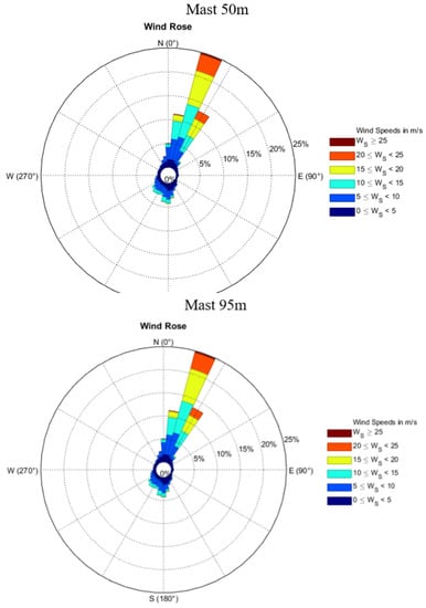
Figure 5.
Wind rose from 1 April 2016 to 1 April 2017 at mast heights of 50 m and 95 m.
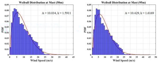
Figure 6.
Weibull distribution from 1 April 2016 to 1 April 2017 at mast heights of 50 m and 95 m.
2.5.3. Wind Turbine
A Siemens SWT-4.0-120 turbine, which conforms to IEC Class IA, was used in this study to evaluate the potential of wind power generation because two turbines of this type were erected in 2016 as demonstration offshore wind turbines in Taiwan. The rated power output of one such turbine is 4 MW at a rated wind speed of 16 m/s. The rotor diameter is 120 m, and the swept area is 11,300 m2.
2.5.4. Park Optimization
WindSim optimizes park layouts by identifying turbine locations with the highest wind speeds but low turbulence to maximize energy production while minimizing turbine load problems. The wake effect is the main parameter in park optimization. The Jenson model was used as wake model used in this study. The decay coefficient, , was set to 0.05 for the offshore condition [45]. With the input of velocity scalar XY, velocity scalar Z, and inflow angle and turbulence intensity at hub height and blade tip height, the Park Optimizer module was used to optimize the wind farm. The limitation of the IEC standard is summarized in Table 3. The Park Optimizer considered the terrain condition, inflow angle, turbulence intensity, and velocity for setting the limitation for turbines. The Park Optimizer calculates the best locations for different numbers of turbines by determining the inter-turbine distance required to avoid the wake effect. For determining turbine locations, inter-turbine distance is calculated with the limitation and the wind resource map, which the files export after performing the CFD calculation and importing terrain data and wind data. The results of the Park Optimizer are the energy production affected by wake effects and turbine coordinates.
Table 3.
Main IEC checks for site conditions and limits.
2.6. Uncertainty in Wind Resource Assessment
Numerous factors influence the forecasting results, such as performance of numerical weather prediction, power curves, and measurements. Wind resources can be classified as historical and future resources. Historical wind resources usually present an uncertainty of 3% to 6%. Without a reference data source or in the absence of thorough data analysis, the uncertainty for one year of measurement is assumed to be 4% [3]. For future wind resources, uncertainty is calculated as follows:
where Np is the number of the years used for estimating uncertainty in the future, and σ is the uncertainty for a year. The uncertainty due to climate change ranges from 0.5% to 2%. Brower et al. indicated that the uncertainty is 0.5% when Np equals 10 years and 2% when Np equals 25 years [3].
For long-term wind prediction, uncertainty is based on the correlation coefficient of the wind speed between the target site and the reference site. Correlation coefficients greater than 0.9, between 0.9 and 0.8, and between 0.7 and 0.6 indicate wind speed correlation uncertainties of less than 1%, between 1% and 2%, and between 3% and 5%, respectively [46].
The power curve is one of main sources of uncertainty. The power output is given for steady wind conditions, while power cannot be generated as ideally as shown by the curve. The main causes of uncertainty are turbulence, air density, and the shear characteristics of the site. The uncertainty of a power curve is usually 6% [47].
Various parameters pertaining to uncertainty have been used to forecast the probability of energy production. P50 represents a 50% probability that a given amount of energy will be generated [48]. The probability of energy production for probability x, Px, is as follows:
where z is the value of normal distribution for a specific probability.
2.7. Economic Evaluation
The number of turbines and their coordinates were obtained using the Park Optimizer. An economic evaluation was conducted to determine the value of the wind farm. The costs of a wind farm include capital and operational expenditures (Table 4). Because Taiwan currently has no commercially operating offshore wind farms, expenditures of offshore wind farms in the United States [49] and Europe [50] were used to conduct economic evaluation of offshore wind farms in the present study.
Table 4.
Expenditures of offshore wind farms in the United States and Europe.
The offshore wind power purchase price in Taiwan decreased slightly from 2017 to 2018 owing to a decrease in costs (Table 5). Calculation results obtained based on this price can be used to estimate whether the development of a wind farm is worthwhile in terms of the values of net present value (NPV) and energy cost.
Table 5.
Wind power purchase price in Taiwan [51,52].
2.7.1. Net Present Value
The NPV represents the difference between the present value of cash inflows and cash outflows over a period of time for an investment. The general formula for calculating NPV is as follows:
where is the net cash inflow during the period t, is the total initial investment, and r is the discount rate.
The formula used in this study is as follows:
where is the fixed cost, is turbine costs, represents variable costs such as cabling and foundation costs, n is number of turbines, is power generation, is price of power sales, and is operational cost. The values of and vary with time. The values of sales or cost for the first year are considerably greater than the corresponding values for the last year.
An investment with a positive NPV is generally regarded as profitable. Based on 4C Offshore data, the target wind farm requires an investment of 4.700 billion US dollars (137.6 billion NTD). The fixed cost , which includes the costs of transformers, wharves, grid connections, and other costs not related to turbines, was estimated as the difference between the total investment and capital expenditure; it was calculated to be 50 billion NTD.
2.7.2. Cost of Energy
The cost of energy is the price of generating energy. The formula used to determine it in this study is as follows:
where the parameters are the same as those for NPV.
3. Results and Discussion
3.1. Potential for Power Generation
The power generation and capacity factor of a 4-MW Siemens SWT-4.0-120 turbine at the mast site were estimated using WindSim with the data measured at the mast. The energy produced in winter was almost four-fold higher than that produced in summer (Figure 7). The average capacity factor of a single turbine was around 41%.
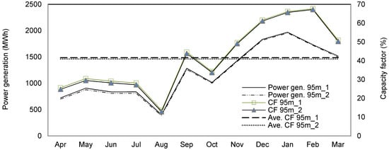
Figure 7.
Power generation and capacity factor of a 4-MW Siemens SWT-4.0-120 turbine from April 2016 to April 2017 at mast site estimated using two sets of measured data at mast height of 95 m.
The AEP and capacity factor with different numbers of turbines in the ZoP 26 wind farm indicated that the AEP increased as the number of turbines increased (Figure 8). For an inter-turbine distance of 12D (D = turbine diameter), the capacity factor was higher than 48.6%. If the distance were to decrease to 6D, the number of turbines would increase to 132 accordingly, while the capacity factor would decrease to 47.6%.
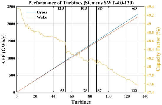
Figure 8.
AEP and capacity factor with different numbers of turbines in ZoP 26 wind farm estimated using mast data.
The AEP under the gross and wake conditions is illustrated in Figure 8. Wake loss increases as the number of turbines increases (Figure 9). The curve of wake loss was not smooth because the simulation was conducted independently for different numbers of turbines. The slope of wake loss increased with the number of wind turbines installed. The wake loss was 3.5% for the inter-turbine distance of 6D compared with the wake loss values obtained by onshore simulation [53] and from offshore floating turbines [54] for various inter-turbine distances.
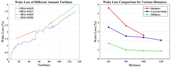
Figure 9.
Wake loss for different numbers of turbines in wind farm and for various inter-turbine distances compared to the values obtained in onshore and offshore simulations.
3.2. Wind Farm Optimization
The NPV analysis of indicated that the purchase price obtained using the stepped purchase price yielded higher profit than that obtained using the continuous value, and the cost of power in Europe was lower than that in the United States (Figure 10). When using continuous purchase price and Europe’s expenditures, 131 turbines would be needed to generate sufficient power to ensure that the NPV is positive. When using the stepped purchase price, only 118 turbines would be needed for a profitable project. The NPV cannot be made positive by using United States’ expenditures, even if the revenue from power sales were calculated using the stepped purchase price. This means that the expenditures of an offshore wind farm would need to be as low as those in Europe to make this investment lucrative.
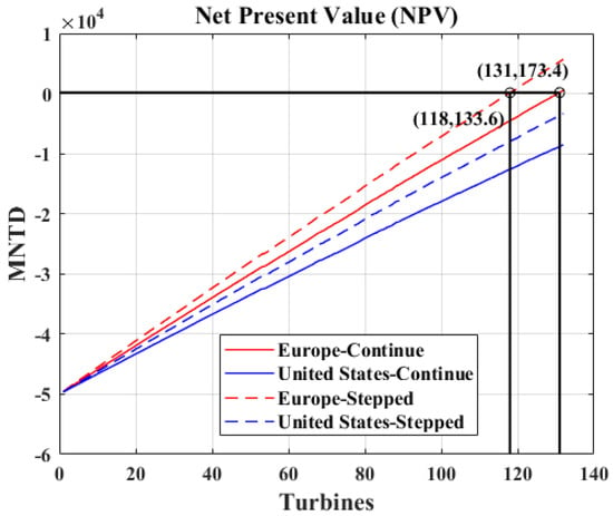
Figure 10.
Net present value for different numbers of turbines considering the purchase price of wind energy in Taiwan.
The analysis of energy cost indicated that the cost is less than 0.1 million NTD/MWh considering Europe’s expenditures and more than 40 turbines (Figure 11). Similar results were obtained considering the United States’ expenditures. In terms of the cost of including additional turbines, the value was less than −0.001 for more than 53 turbines, which means that the cost of including an additional turbine was almost constant.
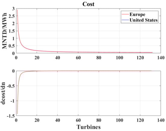
Figure 11.
Cost of energy with different numbers of turbines and the cost of including an additional turbine. The lines of Europe and United States overlap, indicating that the energy cost and the cost of including an additional turbine are similar when calculated using Europe’s and United States’ expenditures. (dcost: additional cost, dn: additional turbine).
Considering that a profitable project required at least 118 turbines, the following energy production was calculated based on wind farm optimization for 118 turbines. The wind farm layouts were optimized using WindSim to identify turbine locations with the highest wind speeds but low turbulence, as well as to maximize energy production and to minimize turbine load problems (Figure 12).
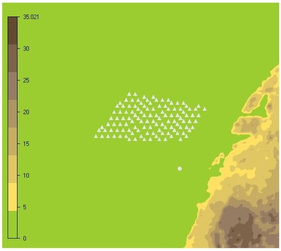
Figure 12.
Turbine layout based on park optimization for 118 turbines.
3.3. Estimating Long-Term Historical Power Production of Wind Farm Using MCP
The power production of ZoP 26 was assessed using measured data and MCP data for long-term prediction. The one-year data measured at the mast from 2016 to 2017 represents the target data of wind resources. The long-term data contained actual and synthesized data for simulating historical wind conditions. Reference data from MERRA and CWB locations Lukang and Shenggang were used to conduct MCP. The one-year simulation used hourly wind speeds and wind directions obtained at the mast heights of 10, 30, 50, and 95 m.
The correlation of wind direction between the two sources must be adequately strong to conduct MCP before the correlation of wind speed between the two sources can be checked. The correlation coefficients of wind direction data between the mast and MERRA 1–4 were 0.782, 0.827, 0.799, and 0.81, respectively. The correlation coefficients between the mast and CWB Lukang and Shenggang were very good at 0.909 and 0.898, respectively (Figure 13). The correlation coefficients of wind speed data between the mast and MERRA 1–4 were 0.316, 0.652, 0.611 and 0.634, respectively. The correlation coefficients between the mast and CWB Shenggang and Lukang were moderate at 0.746 and 0.631, respectively (Figure 13).
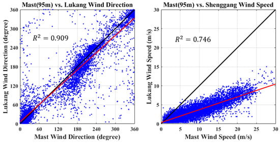
Figure 13.
Correlation coefficient of wind direction data between mast and CWB Lukang (left) and of wind speed data between mast and CWB Shenggang (right).
The aforementioned correlations of wind speeds are overall correlations. MCP for wind speed employs the relationship between two data individually in 12 sectors of wind direction. The correlation coefficient of wind speed between the mast and MERRA and the mast and CWB stations for each sector are listed in Table 6, while the correlation formulas of wind speed for 12 sectors are listed in Table 7. The relationship between the target data and reference data is significant for conducting MCP. The linear least-squares method, a common method for finding the relationship between two data sets, was used in this study to discover the linear equation and coefficients for MCP. The data unavailable at the target site were synthesized using the correlation formula of each sector.
Table 6.
Correlation coefficient of wind speed between mast (95 m) and MERRA 1–4 and CWB Lukang and Shenggang for 12 sectors.
Table 7.
Correlation formulas of wind speed between mast (95 m) and MERRA 1–4 and CWB Lukang and Shenggang for 12 sectors.
The time series of wind speed at the mast (95 m height) (obtained with MCP by using the data measured at the mast and MERRA location 2 as reference data) indicated repeated occurrences of high wind speeds in winter and of low wind speed in summer (Figure 14).
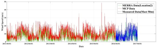
Figure 14.
Time series of wind speed at mast (95 m height) with MCP by using data measured at mast and MERRA location 2.
The Weibull distributions of MCP data obtained from CWB Lukang and the measured mast data are very close (Figure 15), and the distributions of the data recorded at MERRA locations 2, 3, and 4 were similar with the highest probability at the wind speed of 7 m/s.
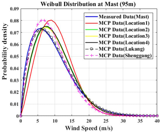
Figure 15.
Weibull distribution at mast (95 m height) describes the probability density of different wind speeds with measured mast data and MCP data obtained using MERRA data of locations 1–4 and CWB data of Lukang and Shenggang.
The AEP of the wind farm was calculated using Equation (1) from Section 2.4 with consideration of wake loss. The AEP values obtained using different numbers of cells did not change significantly when the number of cells was increased from 184,960 to 961,000 (Table 8). Higher levels of energy production were simulated using MCP data derived from MERRA locations 2 and 4.
Table 8.
AEP values obtained for different numbers of meshes and data sources by using data measured at mast, MCP data from MERRA data of locations 2 and 4, and CWB data of Lukang and Shenggeng.
3.4. Prediction of Wind Power Generation and Probability
The probability of AEP is based on uncertainties. Uncertainties of parameters are summarized in Table 9. The constant values are discussed in Section 2.5, and the non-constant values change with various conditions. The uncertainty of long-term correlation was estimated using the interpolation method [46], and the results are summarized in Table 10. The wake effect was calculated using WindSim.
Table 9.
Uncertainties of parameters used in this study.
Table 10.
Uncertainties in long-term correlations of different data sources as determined using MCP data from MERRA data of locations 2 and 4, and CWB data of Lukang and Shenggeng.
As described in Section 2.5.1, the mesh of the terrain was calculated from 184,960 to 961,000 cells to ensure that AEP calculations converged. The number of meshes was used to consider whether the value converged for CFD calculation. The convergence of AEP may confirm that the CFD calculation results are correct. The AEP results converged after the number of meshes was more than 519,840 cells. The AEP of P50 was thus based on the AEP estimated with 519,840 cells. P50 represented the assessment of power production without considering uncertainties, while uncertainties affected the result of energy production at P75 and P90. The predictions of energy production became more conservative with increasing probability value (Figure 16). The AEP predicted for 10 years was slightly higher than that for 25 years (Table 11). The MCP data derived from the outermost offshore MERRA location 4 yielded the highest prediction of energy production for the wind farm in ZoP 26, followed by the more nearshore MERRA location 2. The MCP data from the most inland CWB station of Shenggang yielded the lowest prediction of energy production. The AEP of P90 predicted using the MCP data derived from the CWB data of Lukang at 1732 GWh/y was considerably close to the 1735 GWh/y value predicted using measured mast data.
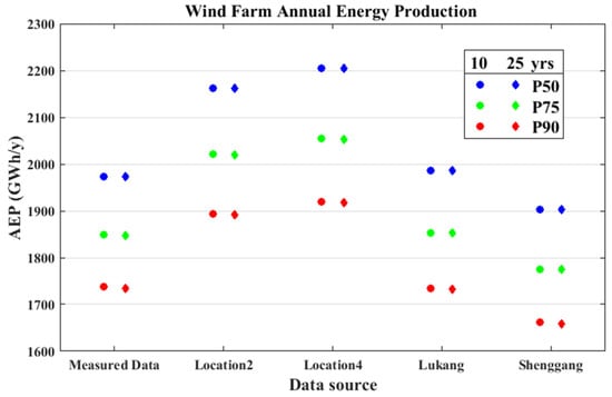
Figure 16.
AEP values of P50, P75, and P90 predicted for 10 and 25 years by using measured mast data, MCP data from MERRA data of locations 2 and 4, and CWB data of Lukang and Shenggeng.
Table 11.
AEP of P50, P75, and P90 predicted for 10 and 25 years using measured mast data, MCP data derived from MERRA data of locations 2 and 4, and CWB data of Lukang and Shenggeng.
Table 12 compares the predicted efficiency of wind farm ZoP 26 for Taiwan, the Netherlands, and the Republic of Korea. The development of offshore wind energy in Taiwan remains in its infancy; domestic wind energy output achieved only 1457 GWh in 2016. The 10-year AEP of P90 predicted using measured mast data at 1737 GWh/y has 119% share of the total domestic wind energy output and 16% of the total domestic renewable energy output. The relatively high percentages indicate the importance of wind farm ZoP 26 for Taiwan. The wind farm has a share of only 0.67% of domestic electricity consumption; therefore, an enormous demand remains for Taiwan to develop offshore wind energy in a transition toward a renewable energy system.
Table 12.
Comparative efficiency of wind farm ZoP 26 for selected countries in 2016.
4. Conclusions
In the present study, we employed multiple data sources to evaluate wind resources and to optimize wind farm design. The vital wind farm optimization findings and energy production predictions are as follows.
When the distance between the turbines in a wind farm was decreased from 12D to 6D, the turbine number increased from 53 to 132, while the capacity factor decreased slightly from 48.6% to 47.6%. The slope of wake loss increased with the number of installed wind turbines. The wake loss reached 3.5% for a turbine distance of 6D. At least 118 turbines would be needed to ensure that the project would be profitable based on NPV evaluation for wind farm optimization.
The AEP predictions became more conservative with increasing probability value from P50 to P90. AEP predicted for 10 years was slightly higher than that for 25 years. MCP data derived from the far-offshore MERRA locations with higher levels of wind resource tended to overestimate the energy production from the target offshore wind farm, which is closer to the coast. MCP data derived from the inland CWB data with lower levels of wind resources tended to underestimate the power generation of the target offshore wind farm. MCP data derived from the inland CWB station with similar levels of wind resources can be used to accurately predict the power generation of the target offshore wind farm, as the results obtained using the data of the CWB station Lukang proved. The use of MCP with mast data as target data, together with CWB and MERRA data as reference data, proved to be a feasible method for predicting offshore wind power generation in places where a mast is available in a neighboring area. For offshore sites, where a mast is not available in a neighboring area, LiDAR can be used to provide short-term measurement data in place of mast data.
The results of this study indicate that the prediction of power generation of the target offshore wind farm was influenced considerably by the wind conditions at the wind measurement site. The higher the level of wind resources was at the wind measurement site, the higher was the predicted power generation of the target offshore wind farm, as indicated by the MCP data derived from MERRA. Similarly, the lower the level of wind resources was at the wind measurement site, the lower was the predicted power generation of the target offshore wind farm, as indicated by the MCP data derived from CWB Shenggang. Using the wind measurement data of a wind resource of similar level as that of the target offshore wind farm, regardless of whether they are mast data or MCP data derived from CWB and MERRA data, can considerably enhance the prediction accuracy of power generation of the target offshore wind farm.
Author Contributions
Conceptualization, C.-D.Y. and T.-H.L.; Data curation, C.-D.Y., C.-C.L. and C.-C.T.; Formal analysis, C.-D.Y. and C.-C.L.; Funding acquisition, T.-H.L.; Investigation, C.-D.Y. and C.-C.L.; Methodology, C.-D.Y. and C.-C.L.; Project administration, C.-D.Y.; Resources, C.-C.T.; Software, C.-D.Y. and C.-C.L.; Supervision, C.-D.Y. and T.-H.L.; Validation, C.-D.Y.; Writing—original draft, C.-D.Y. and C.-C.L.; Writing—review & editing, C.-D.Y.
Funding
This work was carried out under the financial support of the project entitled “Taiwan Offshore Wind Accelerator Roadmap for commercial acceptance of measurement technology” (MOST 106-3113-F-006-002) financed by the Ministry of Science and Technology of the Republic of China.
Acknowledgments
The authors appreciate the support of the project entitled “Development and Application of TPC Offshore Meteorological and Oceanographic Mast Data” (MOST 107-3113-E-006-013-CC2) financed by Ministry of Science and Technology of the Republic of China. The authors also express their appreciation to Taipower for providing measured mast data. This manuscript was edited by Wallace Academic Editing.
Conflicts of Interest
The authors declare no conflict of interest.
References
- 4C Offshore, Global Offshore Wind Speeds Rankings. 2018. Available online: http://www.4coffshore.com/windfarms/windspeeds.aspx (accessed on 24 April 2018).
- Carta, J.A.; Velázquez, S.; Cabrera, P. A review of measure-correlate-predict (MCP) methods used to estimate long-term wind characteristics at a target site. Renew. Sustain. Energy Rev. 2013, 27, 362–400. [Google Scholar] [CrossRef]
- Brower, M. Wind Resource Assessment: A Practical Guide to Developing a Wind Project; John Wiley & Sons: New York, NY, USA, 2012. [Google Scholar]
- Shu, Z.R.; Li, Q.S.; Chan, P.W. Statistical analysis of wind characteristics and wind energy potential in Hong Kong. Energy Convers. Manag. 2015, 101, 644–657. [Google Scholar] [CrossRef]
- Burton, T.; Sharpe, D.; Jenkins, N.; Bossanyi, E. Wind Energy Handbook; John Wiley & Sons: New York, NY, USA, 2001. [Google Scholar]
- European Wind Energy Association (EWEA). Windenergy—The Facts. 2009. Available online: https://windeurope.org/about-us/new-identity/ (accessed on 1 January 2019).
- Andrew. Energy Numbers: Capacity Factors at Danish Offshore Wind Farms. 2018. Available online: http://energynumbers.info/capacity-factors-at-danish-offshore-wind-farms (accessed on 12 April 2018).
- Fuglsang, P.; Thomsen, K. Cost Optimization of Wind Turbines for Large-Scale Offshore WIND farms (No. RISO-R--1000 (EN)); Risø National Lab.: Roskilde, Denmark, 1998. [Google Scholar]
- González, J.S.; Rodriguez, A.G.G.; Mora, J.C.; Santos, J.R.; Payan, M.B. Optimization of wind farm turbines layout using an evolutive algorithm. Renew. Energy 2010, 35, 1671–1681. [Google Scholar] [CrossRef]
- Jiang, B.; Liu, F.; Wang, X.; Du, M.; Xu, H.; Zhang, R.; Ding, J.; Shi, Y.; Cai, X. Research progresses in assessment of China’s offshore wind energy resources. High Technol. Lett. 2016, 26, 808–814. [Google Scholar]
- Pimenta, F.; Kempton, W.; Garvine, R. Combining meteorological stations and satellite data to evaluate the offshore wind power resource of Southeastern Brazil. Renew. Energy 2008, 33, 2375–2387. [Google Scholar] [CrossRef]
- Zheng, C.W.; Li, C.Y.; Pan, J.; Liu, M.Y.; Xia, L.L. An overview of global ocean wind energy resource evaluations. Renew. Sustain. Energy Rev. 2016, 53, 1240–1251. [Google Scholar] [CrossRef]
- Salvação, N.; Soares, C.G. Wind resource assessment offshore the Atlantic Iberian coast with the WRF model. Energy 2018, 145, 276–287. [Google Scholar] [CrossRef]
- Miller, A.; Chang, B.; Issa, R.; Chen, G. Review of computer-aided numerical simulation in wind energy. Renew. Sustain. Energy Rev. 2013, 25, 122–134. [Google Scholar] [CrossRef]
- Charlotte, B.H.; Metrete, B.; Alfredo, P. SAR-Based wind resource statistics in the Baltic Sea. Remote Sens. 2011, 3, 117–144. [Google Scholar]
- Kalnay, E.; Kanamitsu, M.; Kistler, R.; Collins, W.; Deaven, D.; Gandin, L.; Iredell, M.; Saha, S.; White, G.; Woollen, J.; et al. The NCEP/NCAR 40-Year Reanalysis Project. Bull. Am. Meteorol. Soc. 1996, 77, 437–471. [Google Scholar] [CrossRef]
- Uppala, S.M.; KÅllberg, P.W.; Simmons, A.J.; Andrae, U.; da Costa Bechtold, V.; Fiorino, M.; Gibson, J.K.; Haseler, J.; Hernandez, A.; Kelly, G.A.; et al. The ERA-40 reanalysis. Quart. J. Roy. Meteorol. Soc. 2004, 131, 2961–3012. [Google Scholar] [CrossRef]
- Saha, S.; Moorthi, S.; Pan, H.L.; Wu, X.; Wang, J.; Nadiga, S.; Tripp, P.; Kistler, R.; Woollen, J.; Behringer, D.; et al. The NCEP climate forecast system reanalysis. Bull. Am. Meteorol. Soc. 2010, 91, 1015–1057. [Google Scholar] [CrossRef]
- Dee, D.P.; Uppala, S.M.; Simmons, A.J.; Berrisford, P.; Poli, P.; Kobayashi, S.; Andrae, U.; Balmaseda, M.A.; Balsamo, G.; Bauer, P.; et al. The ERA-Interim reanalysis: Configuration and performance of the data assimilation system. Q. J. R. Meteorol. Soc. 2011, 137, 553–597. [Google Scholar] [CrossRef]
- Chadee, X.T.; Clarke, R.M. Large-scale wind energy potential of the Caribbean region using near-surface reanalysis data. Renew. Sustain. Energy Rev. 2014, 30, 45–58. [Google Scholar] [CrossRef]
- Dündar, C.; Inan, D. Investigation of wind energy application possibilities for a specific island (Bozcaada) in Turkey. Renew. Energy 1996, 9, 822–826. [Google Scholar] [CrossRef]
- Lange, B.; Højstrup, J. Evaluation of the wind-resource estimation program WAsP for offshore applications. J. Wind Eng. Ind. Aerodyn. 2001, 89, 271–291. [Google Scholar] [CrossRef]
- Ali, S.M.; Shaban, A.H.; Resen, A.K. Integrating WAsP and GIS Tools for Establishing Best Positions for Wind Turbines in South Iraq. Int. J. Comput. Inf. Technol. 2014, 3, 588–593. [Google Scholar]
- Promsen, W.; Masiri, I.; Janjai, S. Development of microscale wind maps for Phaluay Island, Thailand. Procedia Eng. 2012, 32, 369–375. [Google Scholar] [CrossRef]
- Chantelot, A.; Clarenc, T.; Corrochano, L.; Alegre, M. Meteodyn WT: Site assessment in complex terrain. In Proceedings of the European Wind Energy Conference, Brussels, Belgium, 31 March–3 April 2008. [Google Scholar]
- Gravdahl, A.R.; Harstveit, K. WindSim–Flow Simulations in Complex Terrain, Assessment of Wind Resources along the Norwegian Coast. Available online: https://windsim.com/documentation/papers_presentations/0006_dewek/dewek_2000_proceedings.pdf (accessed on 2 January 2019).
- Berge, E.; Gravdahl, A.R.; Schelling, J.; Tallhaug, L.; Undheim, O. Wind in complex terrain. A comparison of WAsP and two CFD-models. In Proceedings of the European Wind Energy Conference, Athens, Greece, 27 February–2 March 2006. [Google Scholar]
- Albrecht, D.I.C.; Klesitz, M. Three-dimensional wind field calculation above orographic complex terrain in southern Europe. In Proceedings of the European Wind Energy Conference, Athens, Greece, 27 February–2 March 2006. [Google Scholar]
- Llombart, A.; Talayero, A.; Mallet, A.; Telmo, E. Performance analysis of wind resource assessment programs in complex terrain. In Proceedings of the International Conference on Renewable Energy and Power Quality, Palma de Mallorca, Spain, 5–7 April 2006. [Google Scholar]
- Ramsdell, J.V.; Houston, S.; Wegley, H.L. Measurement strategies for estimating long-term average wind speed. Sol. Energy 1980, 25, 495–503. [Google Scholar] [CrossRef]
- Landberg, L.; Myllerup, L.; Rathmann, O.; Petersen, E.L.; Jørgensen, B.H.; Badger, J.; Mortensen, N.G. Wind resource estimation-an overview. Wind Energy 2003, 6, 261–271. [Google Scholar] [CrossRef]
- Justus, C.G.; Mani, K.; Mikhail, A.S. Interannual and month-to-month variations of wind speed. J. Appl. Meteorol. 1998, 18, 913–920. [Google Scholar] [CrossRef]
- Bowen, A.J.; Mortensen, N.G. WAsP Prediction Errors Due to SITE Orography; Risø National Laboratory: Roskilde, Denmark, 2004. [Google Scholar]
- EMD International A/S, WindPRO 2.7 User Guide. 2010. Available online: www.emd.dk (accessed on 20 April 2018).
- Taylor, M.; Mackiewic, P.; Brower, M.C.; Markus, M. An analysis of wind resource uncertainty in energy production estimates. In Proceedings of the European Wind Energy Conference, London, UK, 22–25 November 2004. [Google Scholar]
- Oliver, A.; Zarling, K. The effect of seasonality on wind speed prediction bias in the plains. In Proceedings of the AWEA 2010 Wind Power Conference and Exhibition, Dallas, TX, USA, 23–25 May 2010. [Google Scholar]
- Simisiroglou, N.; Breton, S.-P.; Crasto, G.; Hansen, K.S.; Ivanell, S. Numerical CFD comparison of Lillgrund employing RANS. Energy Procedia 2014, 53, 342–351. [Google Scholar] [CrossRef]
- Castellani, F.; Astolfi, D.; Burlando, M.; Terzi, L. Numerical modelling for wind farm operation assessment in complex terrain. J. Wind Eng. Ind. Aerodyn. 2015, 147, 320–329. [Google Scholar] [CrossRef]
- EWEA, European Wind Energy Association. Comparative Resource and Energy Yield Assessment Procedures Exercise Part II. 2013. Available online: http://www.ewea.org/events/workshops/past-workshops/resource-assessment-2013/ (accessed on 8 March 2018).
- Crasto, G.; Gravdahl, A.R.; Castellani, F.; Piccioni, E. Wake modeling with the Actuator Disc concept. Energy Procedia 2012, 24, 385–392. [Google Scholar] [CrossRef]
- Castellani, F.; Gravdahl, A.; Crasto, G.; Piccioni, E.; Vignaroli, A. A practical approach in the CFD simulation of off-shore wind farms through the actuator disc technique. Energy Procedia 2013, 35, 274–284. [Google Scholar] [CrossRef]
- Lu, C.Y.; Lin, P.H.; Lee, Y.C.; You, Z.C. The measurement of mixing height by Lidar ceilometer at differential landscapes in Taiwan. Atmos. Sci. 2016, 44, 149–171. [Google Scholar]
- Cook, N.J. The Deaves and Harris ABL model applied to heterogeneous terrain. J. Wind Eng. Ind. Aerodyn. 1997, 66, 197–214. [Google Scholar] [CrossRef]
- Drew, D.R.; Barlow, J.F.; Lane, S.E. Observations of wind speed profiles over Greater London, UK, using a Doppler LiDAR. J. Wind Eng. Ind. Aerodyn. 2013, 121, 98–105. [Google Scholar] [CrossRef]
- Hwang, C.; Jeon, J.H.; Kim, G.H.; Kim, E.; Park, M.; Yu, I.K. Modelling and simulation of the wake effect in a wind farm. J. Int. Counc. Electr. Eng. 2015, 5, 74–77. [Google Scholar] [CrossRef]
- Garrad Hassan, GL. Uncertainty Analysis. In WindFarmer Theory Manual; Garrad Hassan, G.L., Ed.; Garrad Hassan & Partners Ltd.: Bristol, UK, 2011; pp. 6–39. [Google Scholar]
- Kwon, S.D. Uncertainty analysis of wind energy potential assessment. Appl. Energy 2010, 87, 856–865. [Google Scholar] [CrossRef]
- Lira, A.; Rosas, P.; Araujo, A.; Castro, N. Uncertainties in the estimate of wind energy production. In Proceedings of the Energy Economics Iberian Conference, Lisbon, Portugal, 4–5 February 2016. [Google Scholar]
- Mone, C.; Hand, M.; Bolinger, M.; Rand, J.; Heimiller, D.; Ho, J. 2015 Cost of Wind Energy Review; National Renewable Energy Laboratory: Golden, CO, USA, 2017. [Google Scholar]
- Valpy, B.; Freeman, K.; Roberts, A. Future Renewable Energy Costs: Offshore Wind; KIC InnoEnergy: Eindhoven, The Netherlands, 2016. [Google Scholar]
- Ministry of Economic Affairs of the Republic of China (MEAROC). 2017 Feed-In Tariff of Electricity Generated from Renewable Energy Sources and Its Calculation Formula; MEAROC: Taipei, Taiwan, 2016. [Google Scholar]
- Ministry of Economic Affairs of the Republic of China (MEAROC). 2018 Feed-In Tariff of Electricity Generated from Renewable Energy Sources and Its Calculation Formula; MEAROC: Taipei, Taiwan, 2017. [Google Scholar]
- Bachhal, A.S. Optimization of Wind Farm Layout Taking Load Constraints into Account. Master’s Thesis, Deparment of Engineering and Science, University of Agder, Kristiansand, Norway, 2017. [Google Scholar]
- Lackner, M. Challenges in Offshore Wind Energy Aerodynamics: Floating Wind Turbines and Wind Farms. The UMass Wind Energy Center. Available online: https://windenergyigert.umass.edu/sites/windenergyigert/files/Lackner%20IGERT%20seminar%20-%20Aerodynamics%20-%203-1-12.pdf (accessed on 12 February 2018).
- IRENA. Renewable Energy Statistics 2018. Available online: https://irena.org/publications/2018/Jul/Renewable-Energy-Statistics-2018 (accessed on 12 February 2019).
- IEA. Key World Energy Statistics 2018. Available online: https://webstore.iea.org/key-world-energy-statistics-2018 (accessed on 12 February 2019).


© 2019 by the authors. Licensee MDPI, Basel, Switzerland. This article is an open access article distributed under the terms and conditions of the Creative Commons Attribution (CC BY) license (http://creativecommons.org/licenses/by/4.0/).