A Data-Driven Predictive Prognostic Model for Lithium-ion Batteries based on a Deep Learning Algorithm

Abstract

Prognostic and health management (PHM) can ensure that a lithium-ion battery is working safely and reliably. The main approach of PHM evaluation of the battery is to determine the State of Health (SoH) and the Remaining Useful Life (RUL) of the battery. The advancements of computational tools and big data algorithms have led to a new era of data-driven predictive analysis approaches, using machine learning algorithms. This paper presents the preliminary development of the data-driven prognostic, using a Deep Neural Networks (DNN) approach to predict the SoH and the RUL of the lithium-ion battery. The effectiveness of the proposed approach was implemented in a case study with a battery dataset obtained from the NASA Ames Prognostics Center of Excellence (PCoE) database. The proposed DNN algorithm was compared against other machine learning algorithms, namely, Support Vector Machine (SVM), k-Nearest Neighbors (k-NN), Artificial Neural Networks (ANN), and Linear Regression (LR). The experimental results reveal that the performance of the DNN algorithm could either match or outweigh other machine learning algorithms. Further, the presented results could serve as a benchmark of SoH and RUL prediction using machine learning approaches specifically for lithium-ion batteries application.

1. Introduction

In the past, nickel–cadmium batteries were generally the only electrical power source for various portable equipment, until nickel metal hybrid and lithium-ion batteries were developed in the 1990s [1]. In the present-day, lithium-ion battery technology is rapidly growing, and it is the most reliable electrical power source for numerous appliances. Lithium-ion batteries are extensively equipped in both high-power applications and low-power electronics products, such as hybrid-motor engines, electric cars, smartphones, tablet, laptops, etc. To date, lithium-ion technology is considered to be a standard power source, and its performance continues to improve. There is currently no any other technology that has proven to perform better than the lithium-ion battery. Therefore, there will be no other battery technologies that lithium-ion anytime soon, and the main focus of the ongoing technology is still aimed at improving the lithium-ion system in term of both its performance and reliability. The following are the main advantages of lithium-ion batteries: (1) high energy density (up to 23–70 Wh/kg), (2) high efficiency (close to 90%), and (3) long life cycle (provides 80% capacity at 3000 cycles) [2].

To ensure that the lithium-ion battery system performing reliably, there must be a method that helps to track and to determine the state of health (SoH) of the battery system, along with its remaining useful life (RUL). This method gives useful information for the prediction of when the battery should be removed or replaced. This type of evaluation is known as the system’s prognostic and health management (PHM). There have been many advancements contributed by researchers from various disciplines to PHM of lithium-ion batteries. Downey et al. proposed a physics-based prognostic approach that considered multiple concurrent degradation mechanisms [3]. Susilo et al. studied the estimation of the lithium-ion battery SoH with the combination of Gaussian distribution data and the least square support vector machines regression approach [4]. Mejdoubi et al. employed the Rao-Blackwellization particle filter to evaluate the aging condition of lithium-ion batteries, and to estimate SoH and RUL of the battery system [5]. Bai et al. developed a generic model-free approach based on ANN and the Kalman filter, to help to improve the health management system of the lithium-ion battery [6]. Other filtering techniques, for example, particle filtering [7] or its variation of the unscented particle filtering technique [8] had been employed in the PHM aspect for lithium-ion batteries. Recently, Li et al. proposed Gauss–Hermite particle filter (GHPF) technique for battery state-of-charge estimation, which is another extension of the particle filter technique, which not only improves the estimation accuracy, but also reduces the number of sampling particles, which reduces the complexity of the algorithm [9]. Another interesting work also aims to predict the health state of the lithium-ion battery, as proposed by Wang et al. This work employed the Brownian motion technique, which is the combination of the Kalman filter and the Gaussian distribution state space technique, to determine battery prognostics based on the drift coefficient [10].

A data-driven model based on the deep learning approach for lithium-ion battery prognostics is the main focus of this paper. Although various approaches had been proposed to improve the PHM prediction of lithium-ion batteries, the deep learning approach for PHM is still limited. The advancement of computational tools and big data algorithms have largely impacted the development of this approach. The machine learning algorithms, in particular, ANN, have been proven to be able to empirically learn and recognize the more complex patterns of the system’s data in many applications. This feature of machine learning algorithms also benefits prognostic analysis modeling as well. This paper presents the preliminary development of a data-driven model using Deep Neural Networks (DNN) to predict the SoH and RUL of lithium-ion batteries. DNN is a deep learning approach that was developed based on Artificial Neural Networks with multiple hidden layers, to analyze more complex data and features. Although some deep learning algorithms, such as Recurrent Neural Network (RNN) and Long Short-Term Memory Network (LSTM), are employed to model prognostic of lithium-ion battery recently, to date, there is no work that has employed a DNN model to perform similar tasks. In addition, there are limited works that have performed a deep learning approach against other data-driven algorithms. For this reason, this paper can also act as a benchmarking reference for employing a deep learning approach to prognostic data in general. The effectiveness of the proposed approach was tested in the lithium-ion battery dataset derived from the NASA Ames Prognostics Center of Excellence (PCoE). A DNN approach was employed to predict the SoH and RUL and the results were compared against other machine learning algorithms such as Linear Regression (LR), k-Nearest Neighbors (k-NN), Support Vector Machine (SVM), and ANN. This paper is constructed with the following sections: Section 2 discusses the overview of the PHM application and the characteristics of the lithium-ion battery used in this paper, Section 3 provides a concise literature review of the proposed approach for DNN analysis and modeling, Section 4 details the experimental results and the comparison of DNN and other machine learning algorithms, and Section 5 concludes the findings and investigates possible future work.

2. Prognostics and Health Management

This paper extends the application of artificial intelligence through machine learning in PHM applications, specifically for lithium-ion battery PHM applications. In this section, an overview of data-driven prognostics and the general prognostic approach for the lithium-ion battery will be discussed briefly.

2.1. Overview of Data-Driven Prognostics

The PHM of the battery has to be included as part of the condition-based maintenance (CBM) plan of the system. The CBM plan is considered as a preventive strategy, which means that maintenance tasks will be performed only when need arises. This need can be determined by continuously evaluating health status of a particular system’s components, or the health state of the system as a whole [11]. CBM has included two major tasks: diagnostics and prognostics. Diagnostics is the process of the identification of faults and part of the current health status of the system, which is described as an SoH, whereas prognostics is the process of forecasting the time to failure. The time left before observing a failure is described as the remaining useful life (RUL) of such a system [12]. To avoid severe negative consequences when systems run until failure, the maintenances must be performed when the system is still up and running. These type of maintenance require early plans and preparation [13]. Thus, CBM must properly be included as part of the system’s operation, especially for the critical systems. The prognostic of the system is a crucial factor in CBM.

The prognostic process additionally involves two phases. The first phase of prognostics aims to assess the current health status or state of health (SoH). Terms that are usually used to describe this phase in most of the literature are severity detection and degradation detection, which can also be considered under diagnostics. Classification or clustering techniques can be utilized to perform tasks such as pattern recognition in this phase. The second phase aims to predict the failure time by forecasting the degradation trend, and by identifying the remaining useful life (RUL). Trend projection, tracking techniques, or time series analysis are included in this phase. Most of the academic articles regarding prognostics analysis only consider the first phase [14]. This paper aims to construct and analyze both SoH and RUL, in which focus is made on both the first and second phases of prognostics for the battery system.

Generally, there are two existing major approaches for prognostics evaluation; the data-driven model, and physics-based models. Data-driven methods require adequate data or samples from systems that were run until failure, while physics-based methods evaluate the system’s failures via the physics of failure progression. Both the data-driven and physics-based model also have different requirements and use cases, and both also have different advantages and drawback as well.

Table 1. Difference between data-driven and physics-based models for diagnostics and prognostics.

	Data-Driven Model [15]	Physics-Based Model [16,17]
Based on	The empirical lifetime data and the use of previous data of the operation of the system	Physical understanding of the physical rules of the system, the exact formulas that represent the system
Advantages	The real behavior of the complex physical system is not required.	Higher accuracy because the model is based on an actual (or near-actual) physical system
	Models are less complex, easier to employ into a real application	The model represents a real system, the model can be observed and judged in a more realistic manner
Drawbacks	Needs a large amount of empirical data in order to construct a high accuracy model	Highly complex, requires extensive computational time/resources, which may not be very suitable for employment in real-world applications
	The models do not represent the actual system, it requires more effort to understand the real system behavior based on the collected data	Limitations in modeling, especially in cases of large and complex systems with non-measurable variables

summarizes the information on the differences and advantages of each model.

One of the data-driven model approaches for prognostics and diagnostics mentioned earlier are machine learning approaches, which will be the main discussion topic of this paper.

2.2. Prognostics of the Lithium-ion Battery

The lithium-ion battery data employed in the prognostics analysis of this work was retrieved from the NASA Ames Prognostics Center of Excellence (PCoE) data repository [18]. This dataset contains the test results of commercially available lithium-ion 1850-sized rechargeable batteries, and the experiment has been performed under controlled conditions in the NASA prognostics testbed [19].

Experimental data were obtained from three different lithium-ion battery-operational test conditions: charge, discharge, and impedance. All experiments were performed at room temperature. The charge was performed at a constant current of 1.5 A until the voltage reached 4.2 V, and then it continued charging at a constant voltage until the charge current dropped to 20 µA. The discharge was also performed at a constant current of 2 A until the voltage dropped to 2.7 V, 2.5 V, 2.2 V, and 2.5 V. These same tests were performed for batteries No. 05, No. 06, No. 07, and No. 18. The impedance test was done by using EIS (Electrochemical Impedance Spectroscopy) frequency adjustment from 0.1 kHz to 5 kHz. By repeatedly performing charge and discharge tests in multiple cycles, this accelerated the aging characteristics of the batteries. This aging effects of the lithium-ion battery can be explained by using the physics-based model established in [20]. The tests were stopped when the batteries reached the end of life criteria, which was defined as a 30% fade from the rated capacity.

Figure 1 is the schematic diagram of the tested battery. The parameters of the schematic diagram included the Warburg impedance (R_W) and the electrolyte resistance (R_E), the charge transfer resistance (R_CT), and the double-layer capacitance (C_DL). The two parameters R_W and C_DL showed a negligible change over the aging process of the battery, and these might be excluded from further analysis [21]. Based on the schematic diagram of the tested battery, below is the characteristic profile of battery No. 05, which will be used as a training data set. Figure 2 shows some details of the current and voltage behaviors during the charging and discharging cycles of battery No. 05. Figure 1 is the schematic diagram of the tested battery. The parameters of the schematic diagram included the Warburg impedance (R_W) and the electrolyte resistance (R_E), the charge transfer resistance (R_CT), and the double-layer capacitance (C_DL). The two parameters RW and C_DL showed a negligible change over the aging process of the battery, and these might be excluded from further analysis [21]. Based on the schematic diagram of the tested battery, below is the characteristic profile of battery No. 05, which will be used as a training data set. Figure 2 shows some details of the current and voltage behaviors during the charging and discharging cycles of battery No. 05.

In order to evaluate the prognostics of the battery, the SoH of the battery must be defined. The prognostics of the battery data are often based on the identification of the SoH of the battery. Therefore, it is important to understand the clear definition of SoH, as the SoH will be the main prediction attribute of the proposed data-driven model, along with RUL. It is also important to note that in this work, all attributes from the test data will be used as training attributes. Some of the attributes (or parameters), and the definition of State of charge (SoC) and SoH in the battery dataset for the prognostics analysis of the battery will be discussed in the following paragraphs.

The SoC of the battery indicates the reliability of the battery system. In the literature, the ratio between the available amount of charge and the maximum amount of charge is commonly referred to as the SoC [6]. In some cases, the available amount of charge can also be replaced by the rated capacity (or nominal capacity) provided by battery manufacturers. The SoC can be mathematically expressed as:

$$Soc=\frac{Q_{available}}{C_N}$$

(1)

where $Q_{available}$ represents the available amount of charge and $C_N$ represents the rated capacity from battery manufacturers.

The SoC definition from Equation (1) seemed to be a straightforward and easy to employ the formula. However, there are some problems using SoC as battery health measurement. First, the only way to derive the rated capacity of a battery is through experiments under a constant discharge rate within a controlled experimental environment. This reason explains the difficulty in using a rated capacity as a reference point in real-world applications [22]. Second, SoC is not considered to have a strong correlation with battery capacity. This is a vital point for making a long-term estimation of the battery’s health, since the capacity is the main indication of the battery’s health, which will fade over time.

Many alternative SoC equations are defined in several studies to address the aforementioned issues. One interesting definition is practical state-of-charge, or SoCN [23]. This definition uses the maximum practical operational capacity, instead of the manufactured rated capacity, as the maximum amount of charge. SoCN can be expressed as:

$$So{C}_N= \frac{Q_{available}}{C_{ max,p}}$$

(2)

where $C_{max,p}$ represents the maximum practical capacity as measured from the operating battery at the current time. $C_{max,p}$ may fade over time, due to the effect of battery aging.

Apart from the different ways of quantifying SoC, SoH is another important parameter for battery health management. SoH is the direct indication of the health condition of the battery system. SoH can be generally defined as:

$$SoH=\frac{C_{max,p}}{C_N}$$

(3)

One of the most important tasks in prognostics health management of a battery is to accurately estimate the $C_{max,p}$, as $C_{max,p}$ is required in both Equations (2) and (3) for SoC and SoH estimations, respectively. Our tested battery dataset contained all the aging information of the battery, and the battery SoH was calculated from cycle 0 to cycle 168. As shown in Figure 3, the estimated SoH of battery No. 05 exponentially degraded as the cycle number increased. The acceptable predicted results must be within the 95% confidence bound [24]. The regression model for SoC and SoH estimation, which aimed to perform similar tasks, was also proposed in [25]. This work introduced a new variable to directly indicate the voltage drop of the battery cell as the prediction variable. This work delivered very interesting results. However, it is not within the scope of our deep learning approach. Our work aimed to use only existing test variables to train and generate the deep learning model for the SoH and RUL estimation of lithium-ion batteries.

As a quantification metric to evaluate the performance of the prediction model in this work, the root mean square error (RMSE) was employed for SoH, and the error of RUL cycle (E_RUL) was employed for RUL. The following are the formulas of RMSE and E_RUL:

$$RMSE=\sqrt{\frac{1}{n}{\displaystyle \sum }_{i=1}^n{\left[x_i-{\overline{x}}_i\right]}^2}$$

(4)

$$E_{RUL}=\left|RU{L}_{real}-RU{L}_{prediction}\right|$$

(5)

where $n$ is the number of prediction datasets,$x_i$is the real value of testing and monitoring the battery capacity, and ${\overline{x}}_i$ is the prediction value. RMSE and E_RUL are used as the key performance measures of the performance of all traditional machine learning approaches and the proposed deep learning algorithm. RMSE and ERUL will be calculated within the testing phase of the modeling framework, which will be discussed in the next section.

3. Data-Driven Prognostic Analysis and Modeling

The reason that the machine learning approach works well with the prognostic data, in general, is due to the condition monitoring system, where it collects massive data from equipment. This large amount of data benefits data-driven PHM models, which requires large empirical data in order to create a high accuracy model of the systems. The traditional machine learning methods, called shallow learning models employed in this paper, include: Linear Regression (LR) [26] with the Akaike Information Criterion (AIC) [27,28], k-NN [29], SVM [30,31], and ANN [32,33,34,35,36]. Although there are multiple machine learning algorithms implemented in this work, the main focus is the concept of deep learning, which will be extensively discussed in this section. The rest of the algorithms are well-documented, and will not be further discussed in this paper. Interested readers are encouraged to refer to the associated references for further information. As the deep learning concept was developed based on the ANN, the first discussion in this section will be an initial description of ANN, then the deep learning algorithm and its applications to prognostics assessments will be discussed accordingly.

3.1. Artificial Neural Networks

An ANN, usually called a neural network, is a mathematical model or computational model that is inspired by the structural and functional aspects of biological neural networks [32]. A single neural network call, or a perceptron, has an interconnected group of artificial neurons, which process computational information by using a connectionist approach from node to node. An ANN is considered to be an adaptive system, which means that it is able to change its shape based on the different structure of information flow gains for the learning phase. Basically, there are two configuration modes in ANN. First are the feed-forward, and second is the back-propagation ANNs. For the feed-forward network, the connections between the units or nodes do not form a completed back-and-forth cycle. Instead, the information in the network moves only one way forward from the input units, through the hidden units, to the output units. Meanwhile, back-propagation moves the information backward, in order to update weights in the network.

Back-propagation is a supervised learning method that has two phases, the propagation phase and the weight update phase [33]. These two phases are repeated until the performance of the network is satisfied. In back-propagation algorithms, the output values from the network are compared with the actual or correct value, through the calculation of the error-function value. This error-function value is fed back through the network as a reference, to make an appropriate adjustment of the weights of each connection. The goal is to reduce the value of the error-function by selecting the proper weights. This process is repeatedly performed in the training cycle until the condition is satisfied. Usually, the network will converge to a certain state where the error of the calculations is small. This scenario can be considered as if the network has the capability to learn a certain target function.

A Multi-Layer Perceptron (MLP) is a feed-forward ANN model that maps multiple sets of input data onto a set of appropriate output. An MLP consists of multiple layers of nodes, with each layer being connected to the next one, except for the input nodes. Each node in MLP is an artificial neuron apply with a nonlinear activation function. MLP employs back-propagation to train the network, while multiple network layers consist of many computational units that are interconnected in a feed-forward fashion. Many applications apply a sigmoid function as an activation function.

There are multiple activation functions that can be implemented in ANN, for example, linear or identity functions, binary step functions, hyperbolic tangent function, and sigmoid function. In this paper, the sigmoid activation function of the hidden layer used in the implementation (Section 4) is a Gaussian spheroid function, expressed as follows:

$$y\left(x\right)=e^{-\left(\frac{{\left|\right|x-c\left|\right|}^2}{2{\sigma }^2}\right)}$$

(6)

The output of the hidden neuron gives a measure of distance between the input vector x and the centroid c of the data cluster. The parameter σ represents the radius of the hypersphere, which is generally determined by using an iterative process of selecting an optimum width. In addition to the activation function of the neural network, another condition that needs to be considered in order to construct the classification model is the learning or training algorithm of the neural network. A learning algorithm is a systematic step-by-step procedure through which the connection weights among the neurons are adjusted to minimize the difference between the predicted and the actual values of an output variable [34]. This adjustment was performed in this study by using the most popular method of training, as mentioned earlier, which is known as the back-propagation learning algorithm. In addition to its broad employments in various applications, the back-propagation learning algorithm has been shown to be more efficient than other learning algorithms for solving most regression problems [35].

There are three main reasons that are impacted by the efficiency of the back-propagation learning algorithm. First, this learning algorithm is simple to perform. Second, the back-propagation learning algorithm is able to provide reasonably accurate results for complicated applications in which the input and output relationships are nonlinear [36]. Finally, and most importantly, the back-propagation learning algorithm has revealed an acceptable level of generalization ability. The performance of the MLP networks trained by the back-propagation learning algorithm is usually controlled by the learning rate and momentum. Varying in a range between 0 and 1, the learning rate is a parameter that affects how the connection weights within a network are updated. These updates also include a portion of the last weight change, to accelerate the training convergence, and to improve the training precision. This portion is defined by the momentum, which, like the learning rate, varies over a range of 0–1. Similar to the number of hidden neurons, a specific rule that determines the best values for the learning rate and momentum has not yet been proposed in the literature. As a result, this determination was performed in this study by examining different values from 0–0.9, with a constant step size of 0.1.

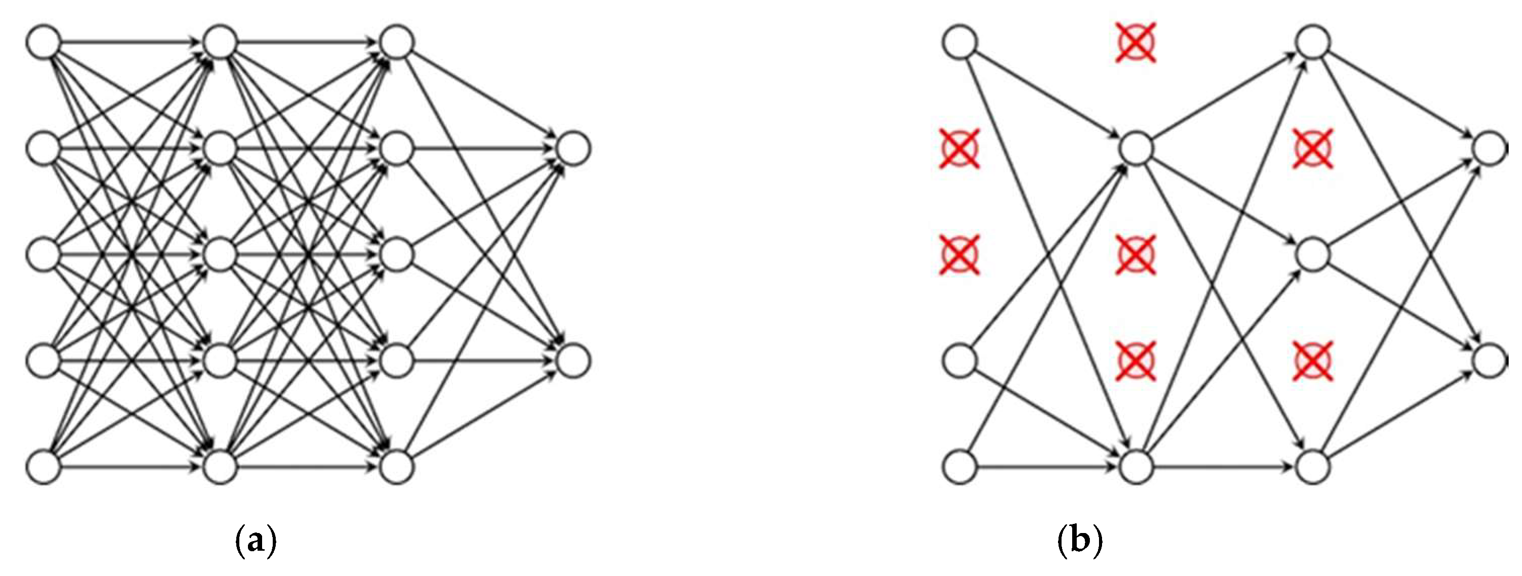
3.2. Overview of the Deep Learning Concept

The deep learning concept was first suggested by Geoffrey Hinton in 2006, and it has become well-known in both academia and industry [37]. Deep learning is an improvement of a Multi-Layer Perceptron with a better power of learning representation, which holds the potential to overcome the deficiencies in traditional machine learning methods [38]. The notable advantage of deep learning is that it is able to capture the representation of information from raw data through multiple complex non-linear transformations and approximations. In order to accurately evaluate the state of systems, to decide whether or not the equipment in the systems need to be maintained or not as part of CBM, fault diagnosis and prognostics may benefit from the utilization of deep learning.

The main algorithms of deep learning include the Deep Neural Network, the Convolutional Neural Network (CNN), the Recurrent Neural Network (RNN), and the expansion of CNN and RNN, such as the Long short-term memory network (LSTM). There are also hybrid networks that combine different types of stacked layers. The following are the characteristics of each deep learning algorithm.

The Deep Neural Network (DNN) is generally a stack of multiple hidden layers instead of only one hidden layer in the standard ANN architecture [39]. The DNN hidden layers are the multiple feed-forward layers that are trained with a back-propagation stochastic gradient descent. The hidden layers consist of neurons nodes with tanh, rectifier (ReLU), and maxout activation functions. DNN has features such as an adaptive learning rate, rate annealing, momentum training, dropout, and regularization. These features are believed to enable a higher predictive accuracy compared to the regular ANN.

The Convolutional Neural Network (CNN) is basically composed of layers of convolutions consisting of neurons, with tanh, ReLU being applied to the results. CNN uses convolutions over the input layer to compute the output. An individual layer of CNN applies different types of filters. The edges of the layers capture the shape of the data, and then they use these shapes to determine higher-level features. The last layer classifies the output by using these high-level features.

The Recurrent Neural Network (RNN) makes use of sequential information. The RNN defines the inputs and outputs as a dependent variable based on a time sequence. RNN performs the same task for every element of a sequence. The output at the last time step of RNN is dependent on the previous computations. RNN may be considered to have a “memory”, as it can capture information about calculations in past sequences. However, RNN has a limitation in capturing the length of the data. This leads to the development of the LSTM network, which can capture longer sequences of information [40,41].

3.3. Employment of Deep Learning to Prognostic Data

In the diagnostics and prognostics fields, the developing trend of employing the deep learning approach has evolved from fault detection and failure diagnosis to degradation pattern recognition and time series predictive analysis. The modeling methods have grown from using only a single algorithm such as DNN, CNN, and RNN, to the Hybrid model, or a combination of multiple layer types and traditional algorithms. The application range of using deep learning has also been expanding continually over the years, from machinery, electrical, and electronics systems, to wind-power and high-end aerospace equipment [38].

In this paper, only DNN was employed to model the SoH and RUL of the battery data against other traditional machine learning algorithms. Each of these deep learning algorithms have their own advantages and disadvantages. It has apparently been discovered that ANN and DNN are more suitable for tackling one-dimensional data. CNN is better handling multidimensional data, as it has adopted types of convolutional techniques. RNN is suitable for applications that deal with time series or dependent input data, and DNN is usually employed for extracting global features from fault data, which will be suitable for the lithium-ion battery data. Additionally, as aforementioned, the layers of CNN and RNN are far more complex than those of DNN. Therefore, CNN and RNN take more time for training the model, which is their major drawback. These reasons make DNN more suitable for employment in real applications for the most case.

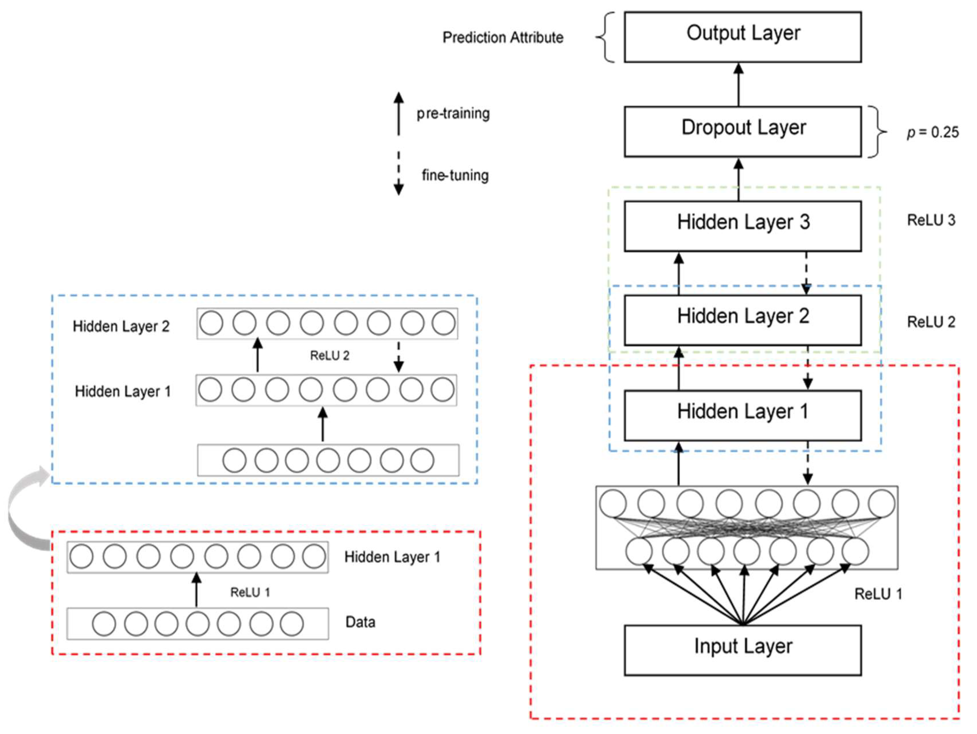
3.4. The Deep Neural Network Framework and Model for Prognostic Data

Currently, deep neural network (DNN) has become a well-employed approach in machine learning, due to its promising performance and advantages. DNN employs a multi-layered feed-forward neural network that is similar to the vanilla artificial neural network, but with densely stacked or fully-connected hidden layers instead of one hidden layer. In order to develop a DNN framework for prognostic data, the similar practice of developing the ANN framework has been used.

In this work, the DNN framework for prognostic data was developed based on a Cross-industry standard process for data mining (CRISP-DM) [42], and this is illustrated in Figure 4. This can be considered as the general framework of fault prognostics by using a deep learning algorithm. The framework is generally divided into five phases: the definition states phase, the pre-processing phase, the training phase, testing phase, and evaluating phase. The details of each phase are as follows:

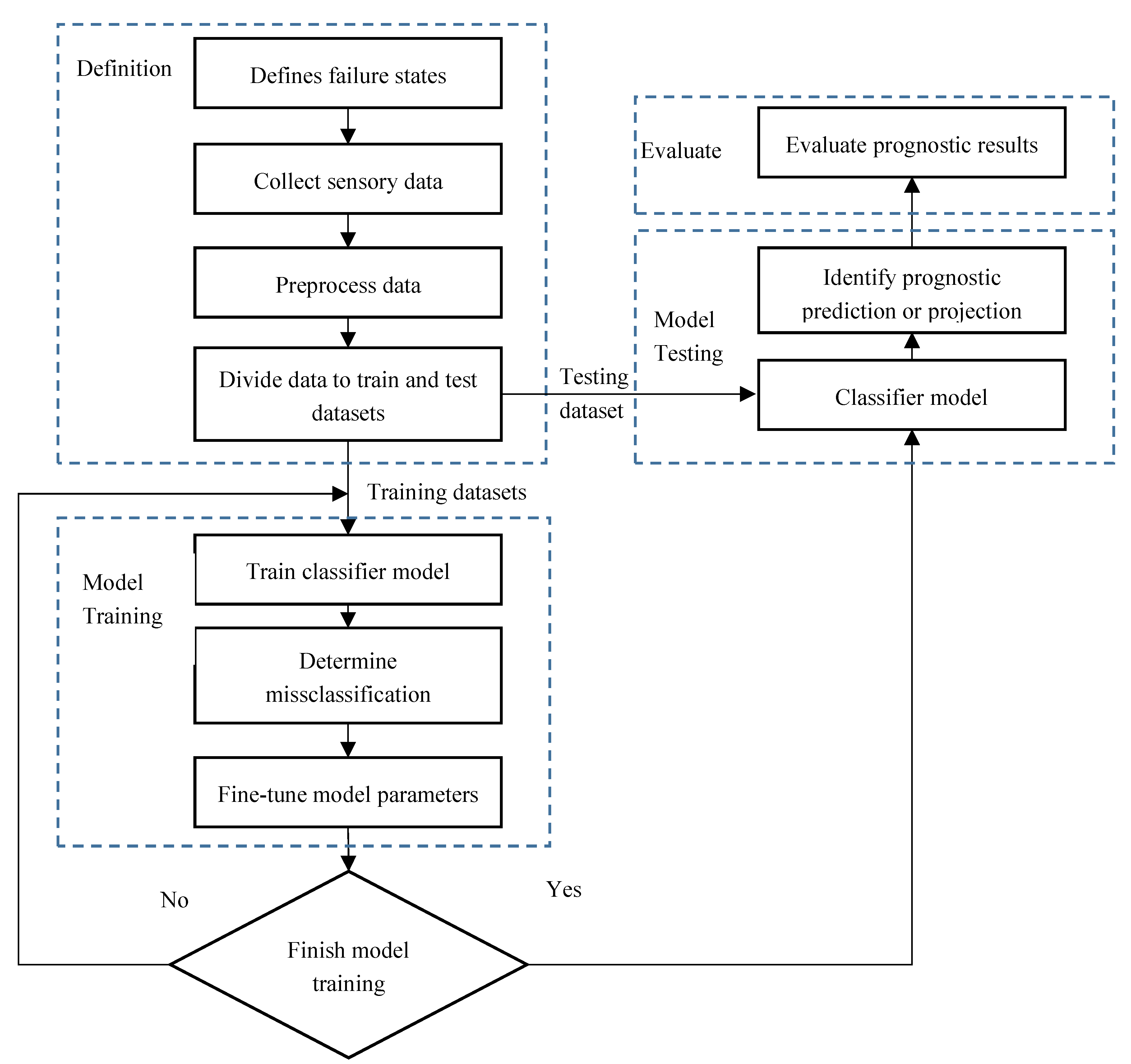
• Definition states phase. This phase specifically focuses on defining the failure of the system, identifying the prognostic problem, and evaluating system health states.
• Pre-processing phase. In this phase, sensory data are collected according to the predefined health state, in order to build a raw dataset for the experiment. The raw datasets are preprocessed and normalized, and then divided into a training and a testing dataset.
• Training phase. In this phase, initial parameters are developed, and the classification model is trained by the training dataset, based on deep learning theory. It is particularly important to fine-tune the classification model through misclassification errors (such as RSME).
• Testing phase. In this phase, the testing dataset is put into the trained classification model to identify prognostic predictions or projection results.
• Evaluating phase. This phase mainly finishes with computing the accuracy, reporting on, and evaluating the diagnosis results from the final model.

The prognostic model of the battery data using DNN was developed based on the aforementioned framework. The experiment with the data was constructed by varying the number of dense layers in DNN. In this experiment, the hidden layer was varied to analyze the SoH of battery data until it delivered the best RMSE results. In addition, the dropout layer was also applied as the last layer before the output layer, to prevent the overfitting problem. The dropout layer applied to the last layer of DNN, to randomly drop neurons during the model training, as shown in Figure 5. Each neuron is retained with a fixed probability, p which is independent of other neurons. The neural network after being sampled, the so-called “thinned” network, will contain only the surviving neurons (Figure 5b).

By training a neural network with some dropouts, the whole network can be trained more often than training regular networks without dropout, because the network is thinned so that it can be trained at less frequency. The network then becomes less sensitive to some specific weights. This results in the network being better at generalization. In this work, a p-value of 0.25 is applied to the network, as suggested, to be the optimal dropout rate for the network to avoid overfitting, but to still maintain the best prediction accuracy [43].

By varying the hidden layers of DNN from two layers to four layers, the RMSE results from

Table 2. RMSE results of each stacked hidden layer model.

Number of Hidden Layers	RMSE
2	3.815
3	3.247
4	3.275

show that the best formation of DNN consists of three stacked dense or fully-connected hidden layers, with the ReLU activation function (see Appendix A for the explanation of the ReLU function), as described in Figure 6. It might also be worthwhile to note that there are some predictions of fluctuation in the DNN model that are implemented by using the Keras library, which is the open source neural network library that is employed in this experiment. Therefore, each DNN experiment was performed with 10 trials. The RMSE results of the final model (three dense layers) are as shown in

Table 3. RMSE results of 10 trials for a model with three stacked hidden layers.

Trials	1	2	3	4	5	6	7	8	9	10
RMSE	3.917	3.877	3.667	3.507	3.487	3.321	3.296	3.253	3.249	3.247

. The best result from the trials was chosen to be the final model.

From this section, the preliminary model of deep learning was developed, based on the deep neural network. The objective of this paper was to prove that the deep learning algorithm outperformed other traditional machine learning algorithms, and ultimately, to provide a complete benchmark of SoH and RUL prediction for the lithium-ion battery. In the next section, the prognostic of the lithium-ion battery data mentioned in Section 2 will be tested by using the machine learning approach, and a deep learning model that has been mentioned previously.

4. Case Study

In this section, an analysis of battery No. 06, No. 07, and No. 18 degradation datasets obtained from NASA Ames Prognostics Center of Excellence (PCoE) database [18] was conducted to validate the effectiveness of the developed DNN approach. The dataset of battery No. 05 was used as a training dataset for all algorithms. A detailed description of the experimental data has been provided in Section 2 and Section 3, along with the validation method for SoH and RUL. The SoH experimental results from tradition machine learning algorithms and the developed DNN will be presented in Section 4.1. The RUL results from the tradition machine learning algorithms and the developed DNN will be shown in Section 4.2, and all results for both the SoH and RUL estimations from all algorithms will be discussed in Section 4.3.

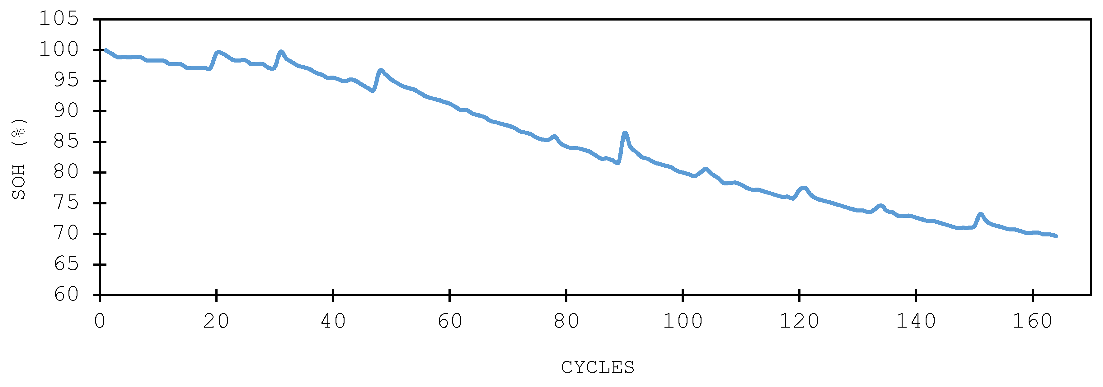
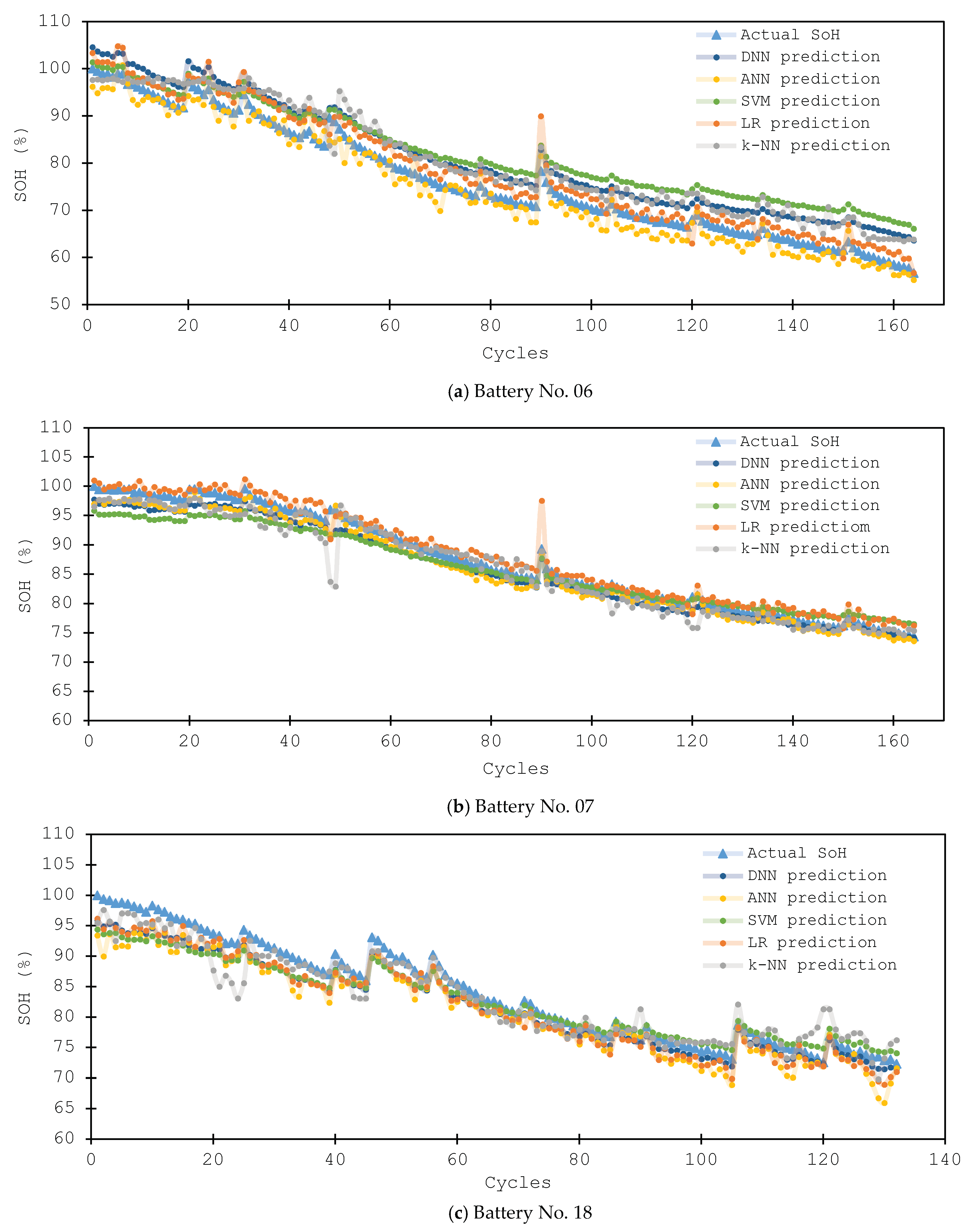
4.1. Results for SoH Estimation

In this experiment, the discharge data for all 164 cycles and 11,345 sample points from battery No. 05 were employed. The SoH was calculated from the initial capacity as being 1.9 AHr. The result is considered to be a long-term SoH estimation of the battery. Figure 7a–c show the SoH estimation performance for batteries No. 06, 07, and 18, using k-NN, LR, SVM, ANN, and DNN respectively. The x-axis represents the cycles, and the y-axis represents the SoH. The triangle marked with a light blue line curve shows the true SoH, and the rest of the curves show the predicted SoH by the k-NN, LR, SVM, ANN, and the developed DNN. The SoH estimators will be employed in each discharge cycle for the SoH estimation.

It might also be worthwhile to mention that the SVM formulation employed in this work was based on the radial basis kernel function, with a regularization parameter of 200, and tolerance-of-loss function of 0.1. LR employed the greedy algorithm with 0.1 minimum tolerance parameters. Additionally, k-NN employed the Euclidean distance measurement to evaluate distances among the neighbor data points.

It is clearly shown in the figures that due to the accurate curve fitting of the trained DNN model with batteries No. 06, 07, and 18, the RMSEs of the SoH estimated by the proposed model are much less than the ones estimated by k-NN, LR, SVM, and ANN. In addition, after the batteries aged from the first cycle to the 164th cycle, it is obvious that the proposed DNN approach could capture the degradation pattern far better than the other algorithms. The input capacity in the developed DNN model could provide sufficient information for the stability of the SoH estimation when the batteries were aged. On the other hand, the lack of the knowledge of other approaches resulted in an increasing error for the SoH estimation in the aged cycles. Furthermore, the performance of the capacity convergence by the proposed DNN approach was better, since the knowledge of capacity fade could be captured better by using the DNN model. Considering the result illustrated in Figure 7, it is also important to note that the results from battery No. 06 performed slightly worse when compared to battery No. 07 and 18. This could be due to the aging pattern of battery No. 06 being slightly different from the training dataset. Additionally, there was a greater distribution of the data of battery No. 06, compared to the other batteries.

The RMSE results between traditional machine learning, k-NN, LR, SVM, and ANN, along with the developed DNN, are shown in Figure 7 and

Table 4. RMSE of the SoH estimation by using DNN and traditional machine learning algorithms.

RMSE	k-NN	LR	SVM	ANN	DNN
	5.598	4.558	4.552	4.611	3.427

. SVM has some drawbacks in terms of capturing the patterns of data; yet, it still outperformed other algorithms based on RMSE. When comparing other algorithms against DNN, DNN was shown to perform the best among the four approaches in terms of capturing both data patterns and RMSE. Additionally, the models constructed from each algorithm could also be observed in detail, from

Table 5. Models created from the training dataset.

Algorithm	Model Description
k-NN	22-Nearest Neighbor model for regression The model contains 624 examples with seven dimensions
LR	228.765 * Voltage_measured + 237.439 × Current_measured − 1.495 * Temperature_measured − 1098.506 × Current_charge + 50.156 * Capacity − 918.727
SVM	Total number of Support Vectors: 613 Bias (offset): −85.065 w[Voltage_measured] = 42686654.125 w[Current_measured] = –17208.396 w[Temperature_measured] = 243822393.316 w[Current_charge] = 3952.097 w[Voltage_charge] = 0.000 w[Time] = 0.000 w[Capacity] = 16430099.458 number of classes: 2 number of support vectors: 613
ANN	Node 1 (Sigmoid) Voltage_measured: –0.172 Current_measured: –0.448 Temperature_measured: 2.894 Current_charge: –1.458 Voltage_charge: 0.005 Time: 0.042 Capacity: –0.155 Bias: –2.726	Node 2 (Sigmoid) Voltage_measured: 1.954 Current_measured: 0.328 Temperature_measured: –1.124 Current_charge: –0.397 Voltage_charge: 0.036 Time: –0.014 Capacity: 0.943 Bias: –1.930		Node 3 (Sigmoid) Voltage_measured: 0.406 Current_measured: 1.254 Temperature_measured: 1.472 Current_charge: 1.391 Voltage_charge: –0.049 Time: –0.036 Capacity: 1.107 Bias: –1.055
	Node 4 (Sigmoid) Voltage_measured: –3.468 Current_measured: –0.975 Temperature_measured: 0.080 Current_charge: –0.018 Voltage_charge: 0.044 Time: –0.020 Capacity: 2.457 Bias: –0.108	Node 5 (Sigmoid) Voltage_measured: –7.072 Current_measured: –0.455 Temperature_measured: 2.095 Current_charge: 2.091 Voltage_charge: –0.004 Time: 0.045 Capacity: –0.464 Bias: –4.078		Output Regression (Linear) Node 1: 1.278 Node 2: 1.460 Node 3: 0.865 Node 4: 1.214 Node 5: –1.134 Threshold: –0.819
	Neural Network created:
DNN	Layer (type)	No. of Hidden Nodes	No. of Parameters	Total parameters: 217 Trainable parameters: 217 Non-trainable parameters: 0
	dense_1 (Dense)	8	64
	dense_2 (Dense)	8	72
	dense_3 (Dense)	8	72
	dropout_1 (Dropout)	8	0
	dense_4 (Dense)	1	9

.

There are some other aspects of the DNN that should also be considered further, which are the optimizer of the network, and the loss function. DNN in this work was performed by employing “Adam” or Adaptive Moment Estimation, as an optimizer (see Appendix B for more details). Additionally, based on the nature of the battery dataset in this work, the absolute error function was employed as the loss function [44]. Absolute errors measured the mean absolute value of the difference between the elementwise inputs. The absolute error formula used as the loss function can be expressed by the following equation:

$$Absolute error loss=\frac{1}{k}{{\displaystyle \sum }}_{i=1}^k{\left|y_i- {\overline{y}}_i\right|}^2$$

(7)

where $y_i$ and ${\overline{y}}_i$ are, respectively, the predicted data and the input data of each iteration or epoch $i$, and k is the number of iterations or epochs. In this work, the total number of iterations or epochs was set to be equal to 1024, as suggested in reference [45].

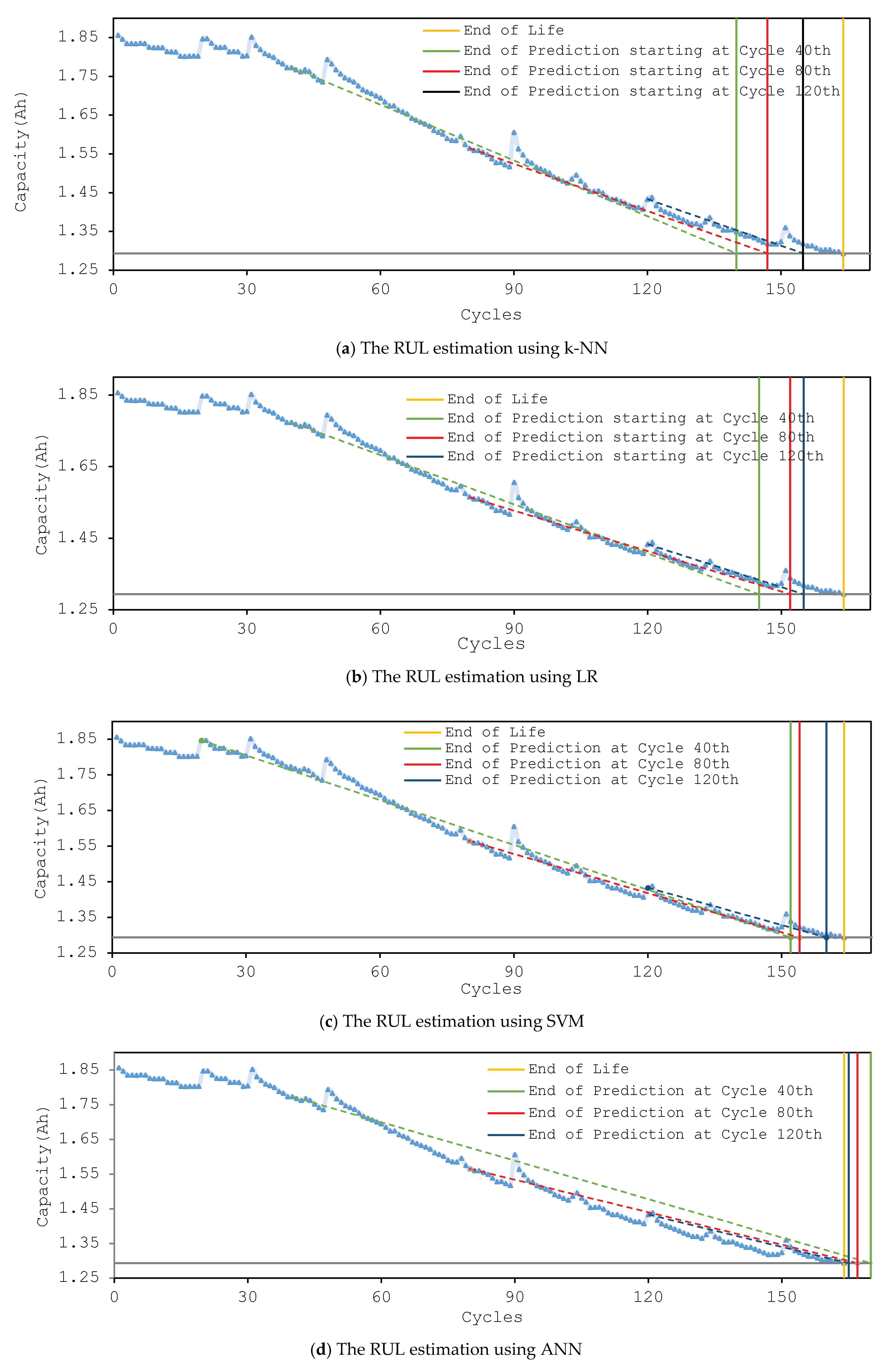
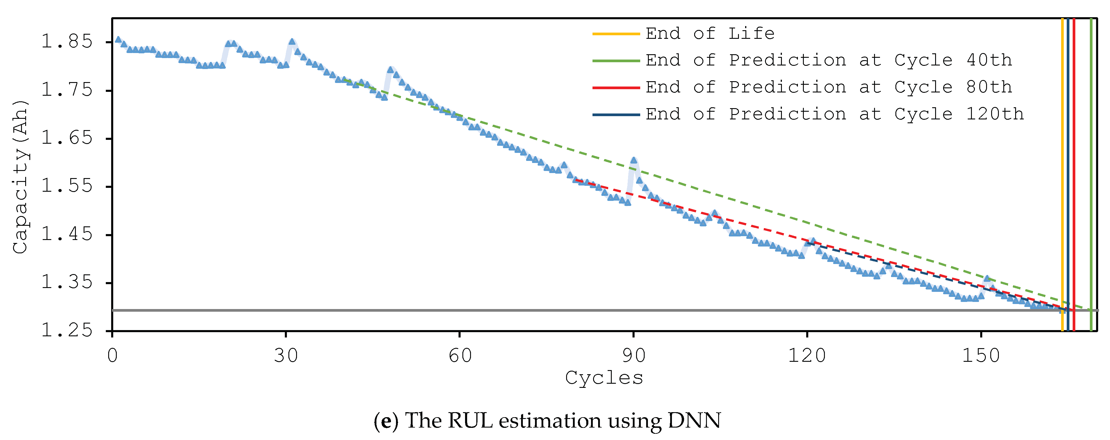
4.2 Results for RUL Estimation

In addition to the SoH prediction of the batteries from the previous section, another aspect of the prognostic analysis of the battery data was to predict the RUL of the batteries. RUL prediction focuses on projecting the degradation results from a certain cycle until the EoL of the batteries, which is different from that of the SoH prediction, which focuses on detecting the pattern of degradation. In this experiment, the goal was to compare the RUL prediction result by using k-NN, LR, SVM, and ANN against the proposed DNN algorithm.

The RUL predictions experiments were performed from three different starting points, which were at the 40th cycle, 80th cycle, and the 120th cycle of battery No. 05. The threshold of the EoL of the battery data was set to be at 30% remaining capacity, or at the 164th cycle. This was deemed to be the rule of thumb of the EoL threshold, for the battery to remain active. The data before the starting cycle was used as a training dataset to make the prediction from each starting cycle, and the error of RUL (Equation (5)) was calculated to compare the accuracy of each machine learning algorithm. The accumulated errors of the RUL results are as shown in

Table 6. The error of RUL estimation by using DNN and traditional machine learning algorithms.

Error of RUL	Starting Points	k-NN	LR	SVM	ANN	DNN
	40th cycle	24	19	12	6	5
	80th cycle	17	12	10	3	2
	120th cycle	19	9	4	1	1

, and the projection results of RUL are as shown in Figure 8. Note that the RUL results focus on making a projection, not to recognize the data’s pattern.

The results from Table 6 and Figure 8 show that, overall, the proposed DNN algorithm outperformed all other machine learning algorithms. The prediction result at the 120th cycle of DNN and ANN are the same. However, DNN still performed better than ANN in term of accuracy while having a smaller set of training data. As shown by the result, DNN provided a slightly better result when starting at the 40th cycle and the 80th cycle. Additionally, the trend of the result also showed that having more training data improves the prediction result for every algorithm in this experiment.

4.3. Discussion and Future Work

From the experimental results in Section 4.1 and Section 4.2, it is obvious that the proposed DNN algorithm can outperform k-NN, LR, SVM, and ANN in these specific lithium-ion battery datasets. However, there are two points that need to be addressed here. First, the DNN proposed in this work can outstandingly capture the degradation pattern based on the prediction of the SoH result in Section 4.1. In contrast, in terms of predicting the projection of the RUL (Section 4.2), the performance of DNN is only comparable to ANN. This is suspected to be due to the fundamentals of DNN being based on ANN. The second point is in the case of having smaller training dataset, the DNN performed better overall. This can be observed from the RUL prediction results. DNN provided better results when started from the smaller amount of training data at the 40th and 80th cycles, compared to the typical neural network.

The results obtained from this work also prove that the deep learning algorithm is effective and suitable for employment for prognostic and diagnostic data modeling, particularly in the prognostics of the battery data set. The prognostic results will eventually aid in condition-based monitoring of maintenance activities, to obtain the best time to replace the batteries without causing a long downtime in the main systems. Based on this experiment, the downsides of using a deep learning algorithm include: (1) a higher computational time and (2) more resources are required by DNN than for the other two algorithms. These drawbacks are also true for other deep learning algorithms as well. This conclusion is that deep learning is more suitable for studies that require a higher accuracy, but which may not be the most suitable for works that need real-time processing. In the battery PHM application, real-time processing is not very crucial, since the prediction should be prior to the end-of-life of the batteries. In addition, with the advancement of the computational tools, the real-time processing concern could be minimized, and the computational time will be improved. In the future, real-time processing might no longer be an issue for implementing deep learning in most PHM cases.

The deep learning model in this paper was only developed based on the Deep Neural Network algorithm (DNN). As mentioned in Section 3.4, there are other more complex deep learning algorithms that have been developed over the years, such as the Convolutional neural network (CNN), the Recurrent neural network (RNN), and the Long short-term memory network (LSTM). These deep learning algorithms will be explored in the field of prognostics analysis in the future. It is also worth noting that some researchers have started to employ the LSTM network for similar battery prognostic data, to predict the remaining useful life (RUL) of the battery [46]. Although this has already been done, it is incomparable to the experiments in this work based on the fact that the experiment on LSTM in the literature implemented a different dataset, and more importantly, the experiment only focused on testing the LSTM network in the model, and did not provide a complete comparison to other models that use traditional machine learning algorithms. This leaves gaps to be explored in the future, particularly with benchmarking all deep learning algorithms.

In addition to benchmarking deep learning approaches with other machine learning algorithms, in the future, physical experiments will be explored, to bridge the gap between data-driven models and physics-based models for PHM applications. Data-driven models will be employed to help in easing the modeling complexity in physics-based models of lithium-ion batteries. Thus, an accurate battery models that mimics models in real-world applications could be obtained without the need for extensive outputs of time and resources. The advancements in artificial intelligence and machine learning algorithms play an important role in defining future approaches in PHM for lithium-ion batteries, as well as many other engineering applications.

5. Conclusions

This work aims to accomplish two tasks. First, a complete benchmarking of the data-driven model by using a machine learning algorithm with the battery prognostic data is made. Second, a preliminary data-driven model is developed by using a deep learning algorithm for the prognostic data. This paper has achieved its goal to aid, as a benchmark, the prognostic data-driven model for battery data using machine learning algorithms, and based on the results from the case studies, it shows that the deep learning algorithm provides a promising outcome for predicting and modeling the prognostic data, especially in the battery prognostic and health management applications. Based on the accuracy archived, we also believe that the traditional physics-based model may be replaced by data-driven models in the near future, in various fields and applications. The reliable data-driven model has many advantages over a traditional physics-based model. The first major advantage is that it overcomes the complexity of the physics-based model. This attribute of less complexity in a data-driven model helps to reduce the involvement of the domain experts in particular fields. In the future, the predictive model might be able to be generated and constructed without any opinion or knowledge from experts at all. The second advantage is that data-driven models can be employed in real-time situations, due to the shorter computational time needed, when compared to physics-based models in general. The last point is that the data-driven model is more cost-effective to construct and to employ in real applications. As an example, a data-driven model can be generated and monitored by using only regular personal computing devices, without the need for exclusive and excessive resources. This future trend of data-driven models is in line with the recent achievement of deep learning algorithms and artificial intelligence. These methodologies are believed to be the main approaches in the further development of data-driven models. However, the accuracy of prediction and the higher performance of using deep learning algorithms also comes with the drawback of higher computational time. With rapid advancements in technology, the computational time could be substantially reduced. The future direction of this work will focus on developing a hybrid-deep learning model that could be universally applicable to multiple types of prognostic data.

References

1. Berecibar, M.; Gandiaga, I.; Villarreal, I.; Omar, N.; Van Mierlo, J.; Van den Bossche, P. Critical review of state of health estimation methods of Li-ion batteries for real applications. Renew. Sustain. Energy Rev. 2016, 56, 572–587. [Google Scholar] [CrossRef]
2. Corey, G.P. Batteries for stationary standby and for stationary cycling applications part 6: Alternative electricity storage technologies. In Proceedings of the Power Engineering Society General Meeting, Toronto, ON, Canada, 13–17 July 2003; Volume 1, pp. 164–169. [Google Scholar]
3. Downey, A.; Lui, Y.H.; Hu, C.; Laflamme, S.; Hu, S. Physics-Based Prognostics of Lithium-Ion Battery Using Non-linear Least Squares with Dynamic Bounds. Reliab. Eng. Syst. Saf. 2019, 182, 1–12. [Google Scholar] [CrossRef]
4. Susilo, D.D.; Widodo, A.; Prahasto, T.; Nizam, M. State of Health Estimation of Lithium-Ion Batteries Based on Combination of Gaussian Distribution Data and Least Squares Support Vector Machines Regression. In Materials Science Forum; Trans Tech Publications: Princeton, NJ, USA, 2018; Volume 929, pp. 93–102. [Google Scholar]
5. El Mejdoubi, A.; Chaoui, H.; Gualous, H.; Van Den Bossche, P.; Omar, N.; Van Mierlo, J. Lithium-ion Batteries Health Prognosis Considering Aging Conditions. IEEE Trans. Power Electron. 2018. [Google Scholar] [CrossRef]
6. Bai, G.; Wang, P.; Hu, C.; Pecht, M. A generic model-free approach for lithium-ion battery health management. Appl. Energy 2014, 135, 247–260. [Google Scholar] [CrossRef]
7. Saha, B.; Goebel, K. Modeling Li-ion battery capacity depletion in a particle filtering framework. In Proceedings of the Annual Conference of the Prognostics and Health Management Society, San Diego, CA, USA, 27 September–1 October 2009; pp. 2909–2924. [Google Scholar]
8. Miao, Q.; Xie, L.; Cui, H.; Liang, W.; Pecht, M. Remaining useful life prediction of lithium-ion battery with unscented particle filter technique. Microelectron. Reliab. 2013, 53, 805–810. [Google Scholar] [CrossRef]
9. Li, B.; Peng, K.; Li, G. State-of-charge estimation for lithium-ion battery using the Gauss-Hermite particle filter technique. J. Renew. Sustain. Energy 2018, 10, 014105. [Google Scholar] [CrossRef]
10. Wang, D.; Tsui, K.L. Brownian motion with adaptive drift for remaining useful life prediction: Revisited. Mech. Syst. Signal Process. 2018, 99, 691–701. [Google Scholar] [CrossRef]
11. Camci, F.; Chinnam, R.B. Health-state estimation and prognostics in machining processes. IEEE Trans. Autom. Sci. Eng. 2010, 7, 581–597. [Google Scholar] [CrossRef]
12. Jennions, I.K. (Ed.) Integrated Vehicle Health Management: Perspectives on an Emerging Field; SAE International: Warrendale, PA, USA, 2011. [Google Scholar]
13. Eker, Ö.F.; Camci, F.; Jennions, I.K. Major challenges in prognostics: Study on benchmarking prognostic datasets. In Proceedings of the First European Conference of the Prognostics and Health Management Society 2012, Cranfield, UK, 25 May 2012. [Google Scholar]
14. Qiu, H.; Lee, J.; Lin, J.; Yu, G. Robust performance degradation assessment methods for enhanced rolling element bearing prognostics. Adv. Eng. Inform. 2003, 17, 127–140. [Google Scholar] [CrossRef]
15. Heng, A.; Zhang, S.; Tan, A.C.; Mathew, J. Rotating machinery prognostics: State of the art, challenges and opportunities. Mech. Syst. Signal Process. 2009, 23, 724–739. [Google Scholar] [CrossRef]
16. Jianhui, L.; Namburu, M.; Pattipati, K.; Qiao, A.L.; Kawamoto, M.A.K.M.; Chigusa, S.A.C.S. Model-based prognostic techniques [maintenance applications]. In Proceedings of the AUTOTESTCON 2003 IEEE Systems Readiness Technology Conference, Anaheim, CA, USA, 22–25 September 2003; pp. 330–340. [Google Scholar]
17. Zhang, H.; Kang, R.; Pecht, M. A hybrid prognostics and health management approach for condition-based maintenance. In Proceedings of the IEEE International Conference on Industrial Engineering and Engineering Management, Hong Kong, China, 8–11 December 2009; pp. 1165–1169. [Google Scholar]
18. Saha, B.; Goebel, K. Battery Data Set, NASA Ames Prognostics Data Repository; NASA Ames: Moffett Field, CA, USA, 2007. Available online: http://ti.arc.nasa.gov/project/prognostic-datarepository (accessed on March 2018).
19. Saha, B.; Goebel, K. Uncertainty management for diagnostics and prognostics of batteries using Bayesian techniques. In Proceedings of the Aerospace Conference, Big Sky, MT, USA, 1–8 March 2008; pp. 1–8. [Google Scholar]
20. He, W.; Pecht, M.; Flynn, D.; Dinmohammadi, F. A Physics-Based Electrochemical Model for Lithium-Ion Battery State-of-Charge Estimation Solved by an Optimised Projection-Based Method and Moving-Window Filtering. Energies 2018, 11, 2120. [Google Scholar] [CrossRef]
21. Saha, B.; Goebel, K.; Christophersen, J. Comparison of prognostic algorithms for estimating remaining useful life of batteries. Trans. Inst. Meas. Control 2009, 31, 293–308. [Google Scholar] [CrossRef]
22. Meissner, E.; Richter, G. Battery monitoring and electrical energy management: Precondition for future vehicle electric power systems. J. Power Sources 2003, 116, 79–98. [Google Scholar] [CrossRef]
23. Santhanagopalan, S.; White, R.E. Online estimation of the state of charge of a lithium ion cell. J. Power Sources 2006, 161, 1346–1355. [Google Scholar] [CrossRef]
24. Liu, D.; Pang, J.; Zhou, J.; Peng, Y. Data-driven prognostics for lithium-ion battery based on Gaussian Process Regression. In Proceedings of the 2012 IEEE Conference on Prognostics and System Health Management (PHM), Beijing, China, 23–25 May 2012; pp. 1–5. [Google Scholar]
25. Huang, S.C.; Tseng, K.H.; Liang, J.W.; Chang, C.L.; Pecht, M.G. An online SOC and SOH estimation model for lithium-ion batteries. Energies 2017, 10, 512. [Google Scholar] [CrossRef]
26. Bianco, A.M.; Martínez, E. Robust testing in the logistic regression model. Comput. Stat. Data Anal. 2009, 53, 4095–4105. [Google Scholar] [CrossRef]
27. Akaike, H. A new look at the statistical model identification. IEEE Trans. Autom. Control 1974, 19, 716–723. [Google Scholar] [CrossRef]
28. Burnham, K.P.; Anderson, D.R. Model Selection and Multimodel Inference: A Practical Information-Theoretic Approach; Springer Science & Business Media: New York, NY, USA, 2003. [Google Scholar]
29. Peterson, L.E. K-nearest neighbor. Scholarpedia 2009, 4, 1883. [Google Scholar] [CrossRef]
30. Zhang, Z.; Gu, L.; Zhu, Y. Intelligent Fault Diagnosis of Rotating Machine Based on SVMs and EMD Method. Open Auto. Control Syst. J. 2013, 5, 219–230. [Google Scholar] [CrossRef]
31. Yang, J.; Zhang, Y.; Zhu, Y. Intelligent fault diagnosis of rolling element bearing based on SVMs and fractal dimension. Mech. Syst. Signal Process. 2007, 21, 2012–2024. [Google Scholar] [CrossRef]
32. Samanta, B. Artificial neural networks and genetic algorithms for gear fault detection. Mech. Syst. Signal Process. 2004, 18, 1273–1282. [Google Scholar] [CrossRef]
33. Hegazy, T.; Fazio, P.; Moselhi, O. Developing practical neural network applications using back-propagation. Comput. Aided Civ. Infrastruct. Eng. 1994, 9, 145–159. [Google Scholar] [CrossRef]
34. Jeon, J. Fuzzy and neural network models for analyses of piles. Ph.D. Thesis, North Carolina State University, Raleigh, NC, USA, 2007. [Google Scholar]
35. Emsley, M.W.; Lowe, D.J.; Duff, A.R.; Harding, A.; Hickson, A. Data modelling and the application of a neural network approach to the prediction of total construction costs. Constr. Manag. Econ. 2002, 20, 465–472. [Google Scholar] [CrossRef]
36. Alex, D.P.; Al Hussein, M.; Bouferguene, A.; Fernando, S. Artificial neural network model for cost estimation: City of Edmonton’s water and sewer installation services. J. Constr. Eng. Manag. 2009, 136, 745–756. [Google Scholar] [CrossRef]
37. Hinton, G.E.; Salakhutdinov, R.R. Reducing the dimensionality of data with neural networks. Science 2006, 313, 504–507. [Google Scholar] [CrossRef] [PubMed]
38. Zhao, G.; Zhang, G.; Ge, Q.; Liu, X. Research advances in fault diagnosis and prognostic based on deep learning. In Proceedings of the Prognostics and System Health Management Conference (PHM-Chengdu), Chengdu, China, 19–21 October 2016; pp. 1–6. [Google Scholar]
39. Schmidhuber, J. Deep learning in neural networks: An overview. Neural Netw. 2015, 61, 85–117. [Google Scholar] [CrossRef]
40. Hochreiter, S.; Schmidhuber, J. Long short-term memory. Neural Comput. 1997, 9, 1735–1780. [Google Scholar] [CrossRef]
41. Graves, A.; Mohamed, A.R.; Hinton, G. Speech recognition with deep recurrent neural networks. In Proceedings of the 2013 IEEE International Conference On Acoustics, Speech and Signal Processing (ICASSP), Vancouver, BC, Canada, 26–31 May 2013; pp. 6645–6649. [Google Scholar]
42. Wirth, R.; Hipp, J. CRISP-DM: Towards a standard process model for data mining. In Proceedings of the 4th International Conference on the Practical Applications of Knowledge Discovery and Data Mining, Manchester, UK, 11–13 April 2000; pp. 29–39. [Google Scholar]
43. Srivastava, N.; Hinton, G.; Krizhevsky, A.; Sutskever, I.; Salakhutdinov, R. Dropout: A simple way to prevent neural networks from overfitting. J. Mach. Learn. Res. 2014, 15, 1929–1958. [Google Scholar]
44. Schorfheide, F. Loss function-based evaluation of DSGE models. J. Appl. Econom. 2000, 15, 645–670. [Google Scholar] [CrossRef]
45. Gupta, S.; Agrawal, A.; Gopalakrishnan, K.; Narayanan, P. Deep learning with limited numerical precision. In Proceedings of the International Conference on Machine Learning, Lille, France, 6–11 July 2015; pp. 1737–1746. [Google Scholar]
46. Zhang, Y.; Xiong, R.; He, H.; Liu, Z. A LSTM-RNN method for the lithium-ion battery remaining useful life prediction. In Proceedings of the Prognostics and System Health Management Conference (PHM-Harbin), Harbin, China, 9–12 July 2017; pp. 1–4. [Google Scholar]
47. Hahnloser, R.H.; Sarpeshkar, R.; Mahowald, M.A.; Douglas, R.J.; Seung, H.S. Digital selection and analogue amplification coexist in a cortex-inspired silicon circuit. Nature 2000, 405, 947. [Google Scholar] [CrossRef]
48. Hahnloser, R.H.; Seung, H.S. Permitted and forbidden sets in symmetric threshold-linear networks. In Proceedings of the Advances in Neural Information Processing Systems, Vancouver, BC, Canada, 3–8 December 2001; pp. 217–223. [Google Scholar]
49. Glorot, X.; Bordes, A.; Bengio, Y. Deep sparse rectifier neural networks. In Proceedings of the Fourteenth International Conference on Artificial Intelligence and Statistics, Ft. Lauderdale, FL, USA, 11–13 April 2011; pp. 315–323. [Google Scholar]
50. Orr, G.B.; Müller, K.R. (Eds.) Neural Networks: Tricks of the Trade; Springer: Berlin/Heidelberg, Germany, 2003. [Google Scholar]
51. Nair, V.; Hinton, G.E. Rectified linear units improve restricted boltzmann machines. In Proceedings of the 27th International Conference on Machine Learning (ICML-10), Haifa, Israel, 21–24 June 2010; pp. 807–814. [Google Scholar]
52. Kingma, D.P.; Ba, J. Adam: A method for stochastic optimization. arXiv, 2014; arXiv:1412.6980. [Google Scholar]
Figure 1. The schematic diagram of the tested battery.
Energies 12 00660 g001
Figure 2. The current and voltage during the discharging and charging of battery No. 05: (a) the current of discharging, (b) the current of charging, (c) the voltage of discharging, and (d) the voltage of charging.
Energies 12 00660 g002
Figure 3. The state of health of battery No. 05.
Energies 12 00660 g003
Figure 4. The process of a prognostic framework using deep learning.
Energies 12 00660 g004
Figure 5. Dropout deep neural network model: (a) A standard network with two hidden layers; (b) the network after applying dropout.
Energies 12 00660 g005
Figure 6. The proposed deep neural network model.
Energies 12 00660 g006
Figure 7. The SoH estimation with all algorithms for battery No. (a) 06, (b) 07, and (c) 18.
Energies 12 00660 g007
Figure 8. The RUL estimation of battery No. 05 using (a) k-NN, (b) LR, (c) SVM, (d) ANN, and (e) DNN.
Energies 12 00660 g008aEnergies 12 00660 g008b