Applying Two-Stage Differential Evolution for Energy Saving in Optimal Chiller Loading

Abstract
:1. Introduction
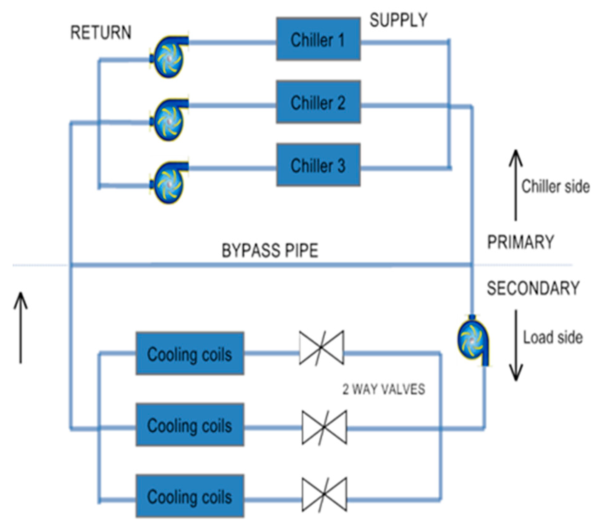
2. Introduction to Multi-chiller System
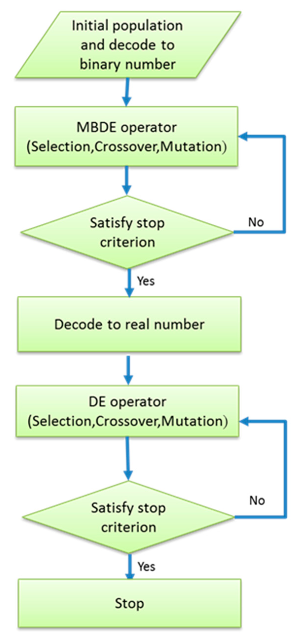
3. Two-Stage Differential Evolution Algorithm
3.1. Differential Evolution Algorithm
3.1.1. Mutation Operator
3.1.2. Crossover Operator
3.1.3. Selection Operator
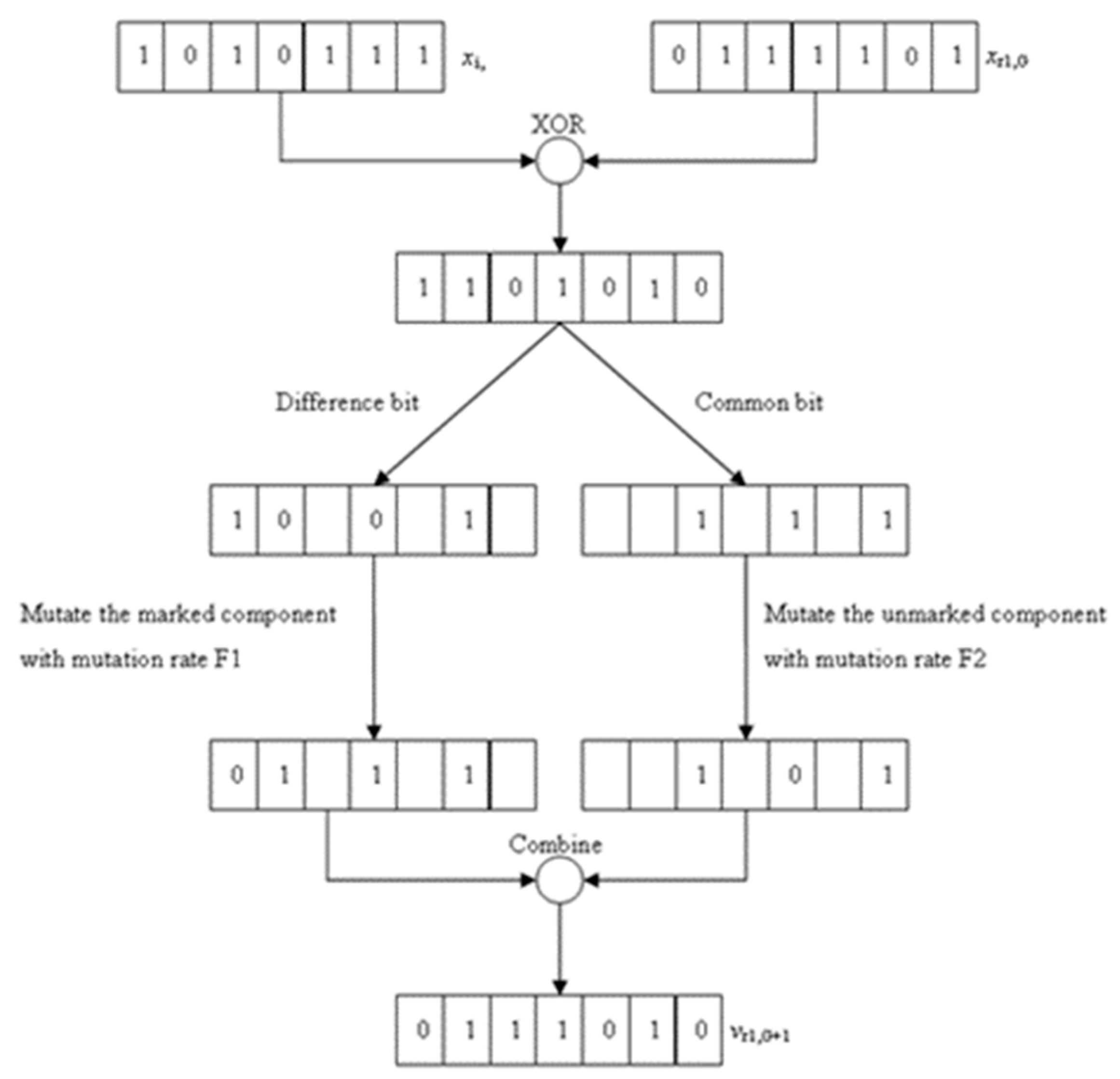
3.2. Modified Binary Differential Evolution (MBDE) Algorithm
3.2.1. Mutation Operator
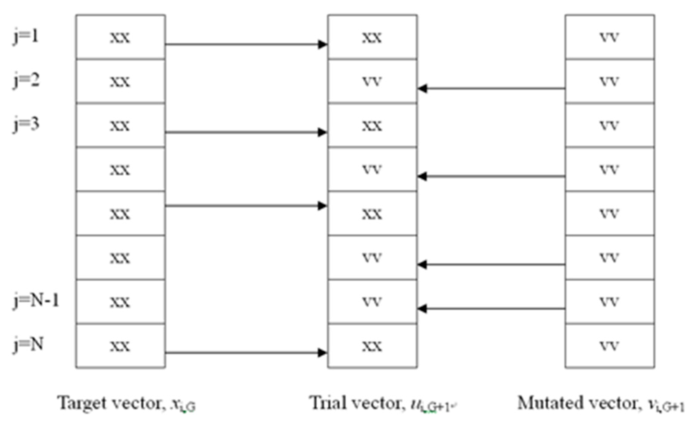
3.2.2. Crossover Operator
3.2.3. Selection Operator
3.3. Two-Stage Differential Evolution Algorithm
4. Results, Analyses and Discussions
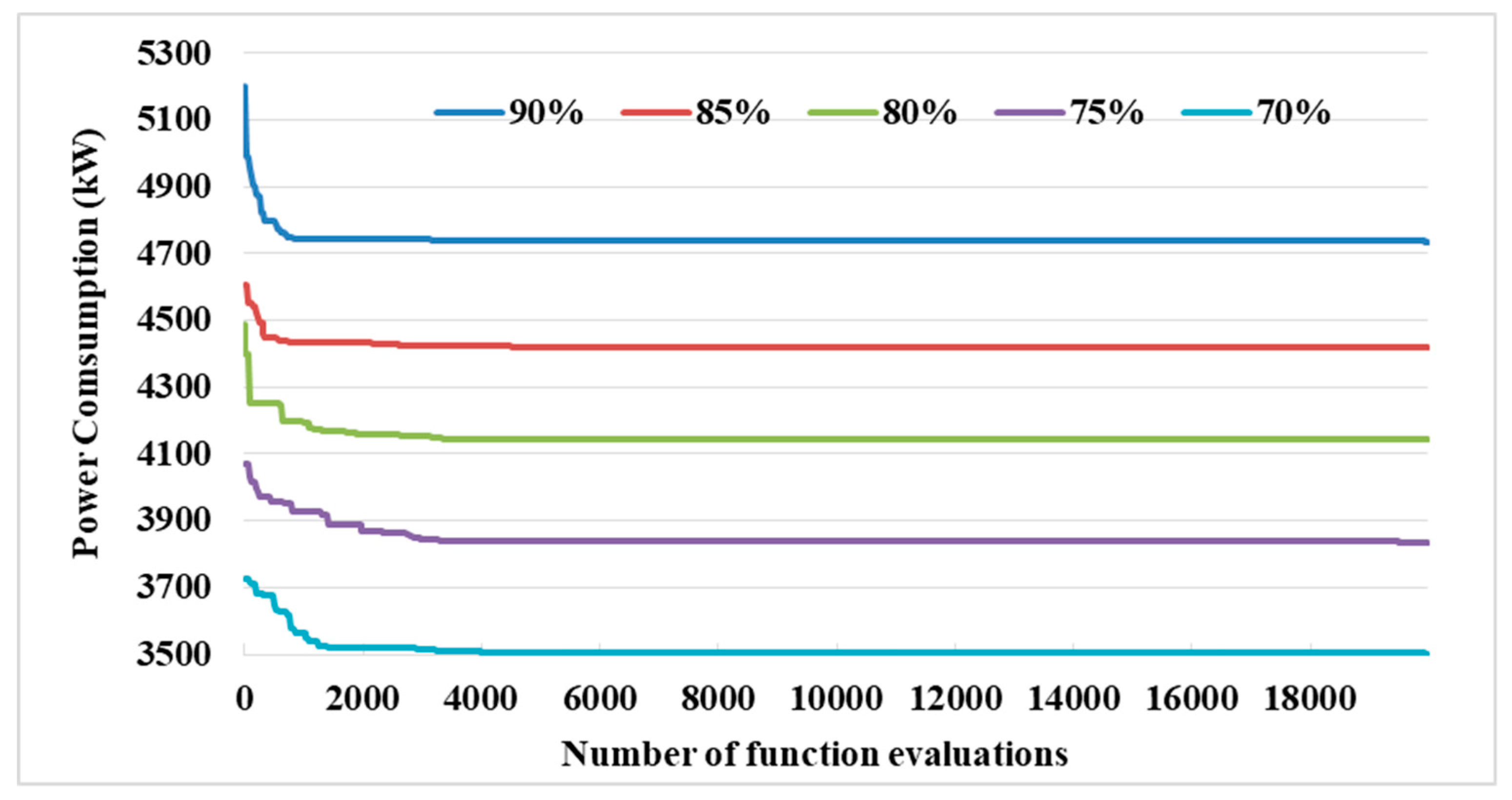
4.1. Case Study 1
4.2. Case Study 2
5. Conclusions
Author Contributions
Funding
Acknowledgments
Conflicts of Interest
References
- Schwedler, M.; Yates, A. Applications Engineering Manual. Multiple-Chiller-System Design and Control; Trane: Dublin, Ireland, 2001. [Google Scholar]
- Chang, Y.C. A novel energy conservation method—Optimal chiller loading. Electr. Power Syst. Res. 2004, 69, 221–226. [Google Scholar] [CrossRef]
- Chang, Y.C.; Lin, F.A.; Lin, C.H. Optimal chiller sequencing by branch and bound method for saving energy. Energy Convers. Manag. 2005, 46, 2158–2172. [Google Scholar] [CrossRef]
- Chang, Y.C. Genetic algorithm based optimal chiller loading for energy conservation. Appl. Therm. Eng. 2005, 25, 2800–2815. [Google Scholar] [CrossRef]
- Chang, Y.C. Optimal chiller loading by evolution strategy for saving energy. Energy Build. 2007, 39, 437–444. [Google Scholar] [CrossRef]
- Ardakani, A.J.; Ardakani, F.F.; Hosseinian, S.H. A novel approach for optimal chiller loading using particle swarm optimization. Energy Build. 2008, 40, 2177–2187. [Google Scholar] [CrossRef]
- Lee, W.S.; Chen, Y.T.; Kao, T. Optimal chiller loading by differential evolution algorithm for reducing energy consumption. Energy Build. 2011, 43, 599–604. [Google Scholar] [CrossRef]
- Coelho, L.D.S.; Klein, C.E.; Sabat, S.L.; Mariani, V.C. Optimal chiller loading for energy conservation using a new differential cuckoo search approach. Energy 2014, 75, 237–243. [Google Scholar] [CrossRef]
- Tan, K.C.; Chiam, S.C.; Mamun, A.A.; Goh, C.K. Balancing exploration and exploitation with adaptive variation for evolutionary multiobjective optimization. Eur. J. Oper. Res. 2009, 197, 701–713. [Google Scholar] [CrossRef]
- Binkley, K.J.; Hagiwara, M. Balancing exploration and exploitation in Particle Swarm Optimization: Velocity-based Reinitializaton. Inf. Media Technol. 2008, 3, 103–111. [Google Scholar] [CrossRef]
- Epitropakis, M.G.; Plagianakos, V.P.; Vrahatis, M.N. Balancing the exploration and exploitation capabilities of the Differential Evolution Algorithm. In Proceedings of the 2008 IEEE Congress on Evolutionary Computation (IEEE World Congress on Computational Intelligence), Hong Kong, China, 1–6 June 2008; pp. 2686–2693. [Google Scholar]
- Bao, H. A Two-Phase Hybrid Optimization Algorithm for Solving Complex Optimization Problems. Int. J. Smart Home 2015, 9, 27–36. [Google Scholar] [CrossRef]
- Beghi, A.; Cecchinato, L.; Rampazzo, M. A multiphase genetic algorithm for the efficient management of multichiller systems. Energy Convers. Manag. 2011, 52, 1650–1661. [Google Scholar] [CrossRef]
- Cheng, M.; Tran, D. Two-Phase Differential Evolution for the Multiobjective Optimization of Time–Cost Tradeoffs in Resource-Constrained Construction Projects. IEEE Trans. Eng. Manag. 2014, 61, 450–461. [Google Scholar] [CrossRef]
- Wu, C.Y.; Tseng, K.Y. Topology optimization of structures using modified binary differential evolution. Struct. Multidiscip. Optim. 2010, 42, 939–953. [Google Scholar] [CrossRef]
- Wu, C.Y.; Tseng, K.Y. Stress-based binary differential evolution for topology optimization of structures. Proc. Inst. Mech. Eng. Part C J. Mech. Eng. Sci. 2010, 224, 443–457. [Google Scholar] [CrossRef]
- Okabe, T.; Jin, Y.; Sendhoff, B. Combination of Genetic Algorithms and Evolution Strategies with Self-adaptive Switching. In Multi-Objective Memetic Algorithms; Springer: Berlin/Heidelberg, Germany, 2009; pp. 281–307. [Google Scholar]
- Storn, R.; Price, K. Differential evolution—A simple and efficient heuristic for global optimization over continuous spaces. J. Glob. Optim. 1997, 11, 341–359. [Google Scholar] [CrossRef]
- Wu, C.Y.; Tseng, K.Y. Engineering Optimization Using Modified Binary Differential Evolution Algorithm. In Proceedings of the Third International Joint Conference on Computational Science and Optimization, Huangshan, China, 28–31 May 2010; pp. 501–505. [Google Scholar]
- Chang, Y.C. An innovative approach for demand side management—Optimal chiller loading by simulated annealing. Energy 2006, 31, 1883–1896. [Google Scholar] [CrossRef]


| Chiller | Rated RT | |||
|---|---|---|---|---|
| 1 | 399.345 | −122.12 | 206.30 | 1280 |
| 2 | 287.116 | 80.04 | 700.48 | 1280 |
| 3 | −120.505 | 1525.99 | −502.14 | 1280 |
| 4 | −19.121 | 898.76 | −98.15 | 1280 |
| 5 | −95.029 | 1202.39 | −352.16 | 1280 |
| 6 | 191.75 | 224.86 | 524.04 | 1280 |
| CL | Algorithm | MIN (kW) | Average (kW) | Max (kW) | SD |
|---|---|---|---|---|---|
| 6868 (90%) | Two-stage DE | 4738.575 | 4733.575 | 4738.575 | 3.919x10⁻⁶ |
| DCSA | 4738.575 | 4738.575 | 4738.575 | 5.313 × 10⁻⁷ | |
| 6477 (85%) | Two-stage DE | 4421.649 | 4421.649 | 4421.650 | 6.355 × 10⁻⁵ |
| DCSA | 4421.649 | 4421.650 | 4421.650 | 2.301 × 10⁻⁴ | |
| 6096 (80%) | Two-stage DE | 4143.706 | 4143.709 | 4143.714 | 3.211 × 10⁻⁴ |
| DCSA | 4143.706 | 4143.710 | 4143.709 | 4.299 × 10⁻⁴ | |
| 5717 (75%) | Two-stage DE | 3838.208 | 3838.217 | 3838.225 | 6.702 × 10⁻⁴ |
| DCSA | 3840.055 | 3840.458 | 3843.766 | 9.428 × 10⁻¹ | |
| 5334 (70%) | Two-stage DE | 3507.270 | 3507.278 | 3507.302 | 1.356 × 10⁻³ |
| DCSA | 3507.270 | 3507.715 | 3511.760 | 1.036 |
| CL | Chiller No. | SA [20] | Power (kW) | PSO [6] | Power (kW) | DCSA [8] | Power (kW) | Two Stage DE | Power (kW) |
|---|---|---|---|---|---|---|---|---|---|
| i | PLRi | of | PLRi | of | PLRi | of | PLRi | of | |
| 6898 (90%) | 1 | 0.7789 | 4777.03 | 0.8026 | 4739.53 | 0.812726 | 4738.575 | 0.81273 | 4738.5750 |
| 2 | 0.7587 | 0.7799 | 0.749619 | 0.749554 | |||||
| 3 | 0.9791 | 0.9996 | 1.000000 | 1.000000 | |||||
| 4 | 0.9781 | 0.9998 | 1.000000 | 1.000000 | |||||
| 5 | 0.9820 | 0.9999 | 1.000000 | 1.000000 | |||||
| 6 | 0.9265 | 0.8183 | 0.838559 | 0.838621 | |||||
| 6477 (85%) | 1 | 0.8051 | 4453.67 | 0.7606 | 4423.04 | 0.727731 | 4421.649 | 0.720409 | 4421.6486 |
| 2 | 0.6056 | 0.6555 | 0.656132 | 0.634290 | |||||
| 3 | 0.9689 | 1.0000 | 1.000000 | 1.000000 | |||||
| 4 | 0.9941 | 1.0000 | 1.000000 | 1.000000 | |||||
| 5 | 0.9866 | 1.0000 | 1.000000 | 1.000000 | |||||
| 6 | 0.7432 | 0.6835 | 0.716524 | 0.746387 | |||||
| 6096 (80%) | 1 | 0.5635 | 4178.73 | 0.6591 | 4147.69 | 0.642735 | 4143.706 | 0.642368 | 4143.7064 |
| 2 | 0.5743 | 0.5798 | 0.562645 | 0.562711 | |||||
| 3 | 0.9675 | 0.9991 | 1.000000 | 0.999999 | |||||
| 4 | 0.9798 | 0.9979 | 1.000000 | 0.999999 | |||||
| 5 | 0.9845 | 0.9921 | 1.000000 | 0.999999 | |||||
| 6 | 0.7338 | 0.5710 | 0.594490 | 0.594798 | |||||
| 5717 (75%) | 1 | 0.6140 | 3925.51 | 0.7713 | 3921.07 | 0.843697 | 3840.055 | 0.843243 | 3838.2079 |
| 2 | 0.4429 | 0.7177 | 0.783794 | 0.783222 | |||||
| 3 | 0.9891 | 0.3000 | 0.000001 | 0.000000 | |||||
| 4 | 0.8867 | 0.9991 | 1.000000 | 0.999999 | |||||
| 5 | 0.9841 | 1.0000 | 1.000000 | 0.999999 | |||||
| 6 | 0.587S | 0.7187 | 0.883049 | 0.882499 | |||||
| 5334 (70%) | 1 | 0.6265 | 3675.34 | 0.6418 | 3642.55 | 0.749969 | 3507.270 | 0.758176 | 3507.269 |
| 2 | 0.7403 | 0.6621 | 0.682477 | 0.689668 | |||||
| 3 | 0.3093 | 0.3301 | 0.000012 | 0.000000 | |||||
| 4 | 0.9546 | 0.9906 | 1.000000 | 1.000000 | |||||
| 5 | 0.9511 | 0.9990 | 1.000000 | 1.000000 | |||||
| 6 | 0.6250 | 0.5806 | 0.776363 | 0.760606 |
| Chiller | Rated RT | ||||
|---|---|---|---|---|---|
| 1 | 104.09 | 166.57 | −430.13 | 512.53 | 450 |
| 2 | −67.15 | 1177.79 | −2174.53 | 1456.53 | 450 |
| 3 | 384.71 | −779.13 | 1151.42 | −63.2 | 1000 |
| 4 | 541.63 | 413.48 | −3626.5 | 4021.41 | 1000 |
| CL | Algorithm | MIN (kW) | Average (kW) | Max (kW) | SD |
|---|---|---|---|---|---|
| 2610 (90%) | Two-Stage DE | 1857.297 | 1858.031 | 1859.626 | 1.317 × 10⁻¹ |
| DCSA | 1857.299 | 1857.315 | 1857.401 | 2.329 × 10⁻² | |
| 2320 (80%) | Two-Stage DE | 1458.334 | 1458.344 | 1458.931 | 2.130 × 10⁻² |
| DCSA | 1455.665 | 1455.810 | 1458.478 | 5.303 × 10⁻¹ | |
| 2030 (70%) | Two-Stage DE | 1178.138 | 1178.928 | 1182.952 | 0.2006 |
| DCSA | 1178.137 | 1181.067 | 1199.495 | 4.803 | |
| 1740 (60%) | Two-Stage DE | 942.050 | 976.182 | 1001.170 | 4.9418 |
| DCSA | 942.183 | 972.076 | 1008.493 | 25.721 | |
| 1450 (50%) | Two-Stage DE | 752.963 | 759.612 | 792.907 | 1.851 |
| DCSA | 753.004 | 765.340 | 824.347 | 17.429 | |
| 1160 (40%) | Two-Stage DE | 583.938 | 630.990 | 661.460 | 3.985 |
| DCSA | 583.923 | 644.933 | 726.016 | 44.015 |
| CL | Chiller No. | GA [4] | Power (kW) | DE [7] | Power (kW) | PSO [6] | Power (kW) | DCSA [8] | Power (kW) | Two Stage DE | Power (kW) |
|---|---|---|---|---|---|---|---|---|---|---|---|
| i | PLRi | of | PLRi | of | PLRi | of | PLRi | of | PLRi | of | |
| 2610 (90%) | 1 | 0.990000 | 1862.18 | 0.99000 | 1857.30 | 0.990000 | 1857.30 | 0.990988 | 1857.299 | 0.990491 | 1857.297 |
| 2 | 0.950000 | 0.91000 | 0.910000 | 0.905473 | 0.905503 | ||||||
| 3 | 1.000000 | 1.000000 | 1.000000 | 1.000000 | 1.000000 | ||||||
| 4 | 0.740000 | 0.760000 | 0.760000 | 0.756593 | 0.756791 | ||||||
| 2320 (85%) | 1 | 0.860000 | 1457.23 | 0.830000 | 1455.66 | 0.830000 | 1455.66 | 0.828756 | 1455.665 | 0.822981 | 1455.733 |
| 2 | 0.810000 | 0.810000 | 0.810000 | 0.805457 | 0.801856 | ||||||
| 3 | 0.880000 | 0.900000 | 0.900000 | 0.896722 | 0.885369 | ||||||
| 4 | 0.6900D0 | 0.690000 | 0.690000 | 0.687883 | 0.685549 | ||||||
| 2030 (70%) | 1 | 0.660000 | 1183.80 | 0.730000 | 1178.14 | 0.730000 | 1178.14 | 0.773478 | 1178.137 | 0.725289 | 1178.138 |
| 2 | 0.760000 | 0.740000 | 0.740000 | 0.739801 | 0.739752 | ||||||
| 3 | 0.760000 | 0.720000 | 0.720000 | 0.721146 | 0.722185 | ||||||
| 4 | 0.640000 | 0.650000 | 0.650000 | 0.627878 | 0.648549 | ||||||
| 1740 (60%) | 1 | 0.600000 | 1001.62 | 0.600000 | 998.53 | 0.600000 | 998.53 | 0.767678 | 942.183 | 0.745135 | 942.059 |
| 2 | 0.700000 | 0.660000 | 0.660000 | 0.004531 | 0.000000 | ||||||
| 3 | 0.510000 | 0.560000 | 0.560000 | 0.746317 | 0.748647 | ||||||
| 4 | 0.590000 | 0.610000 | 0.610000 | 0.646189 | 0.656017 | ||||||
| 1450 (50%) | 1 | 0.600000 | 907.72 | 0.610000 | 820.07 | 0.610000 | 820.07 | 0.515832 | 753.004 | 0.599201 | 752.963 |
| 2 | 0.360000 | 0.000000 | 0.000000 | 0.000001 | 0.000000 | ||||||
| 4 | 0.440000 | 0.570000 | 0.570000 | 0.610547 | 0.S71431 | ||||||
| 4 | 0.580000 | 0.610000 | 0.610000 | 0,607328 | 0.656017 | ||||||
| 1160 (40%) | 1 | 0.330000 | 856.30 | 0.000000 | 651.07 | 0.000000 | 651.07 | 0,000000 | 583.923 | 0.000000 | 583.938 |
| 2 | 0.320000 | 0.000000 | 0.000000 | 0.000014 | 0.000012 | ||||||
| 3 | 0.320000 | 0.560000 | 0.560000 | 0.570369 | 0.556082 | ||||||
| 4 | 0.540000 | 0.600000 | 0.600000 | 0.589625 | 0.603912 |
© 2019 by the authors. Licensee MDPI, Basel, Switzerland. This article is an open access article distributed under the terms and conditions of the Creative Commons Attribution (CC BY) license (http://creativecommons.org/licenses/by/4.0/).
Share and Cite
Lin, C.-M.; Wu, C.-Y.; Tseng, K.-Y.; Ku, C.-C.; Lin, S.-F. Applying Two-Stage Differential Evolution for Energy Saving in Optimal Chiller Loading. Energies 2019, 12, 622. https://doi.org/10.3390/en12040622
Lin C-M, Wu C-Y, Tseng K-Y, Ku C-C, Lin S-F. Applying Two-Stage Differential Evolution for Energy Saving in Optimal Chiller Loading. Energies. 2019; 12(4):622. https://doi.org/10.3390/en12040622
Chicago/Turabian StyleLin, Chang-Ming, Chun-Yin Wu, Ko-Ying Tseng, Chih-Chiang Ku, and Sheng-Fuu Lin. 2019. "Applying Two-Stage Differential Evolution for Energy Saving in Optimal Chiller Loading" Energies 12, no. 4: 622. https://doi.org/10.3390/en12040622
APA StyleLin, C.-M., Wu, C.-Y., Tseng, K.-Y., Ku, C.-C., & Lin, S.-F. (2019). Applying Two-Stage Differential Evolution for Energy Saving in Optimal Chiller Loading. Energies, 12(4), 622. https://doi.org/10.3390/en12040622