Abstract
With the carbon reduction targets being set in the Paris Agreement on Climate Change, China is facing great pressure to meet its emission reduction commitment. The electric power industry as the major source of carbon emissions needs to be a focus. However, the uncertainty of power systems, the risk of reducing emissions and the fuzziness of carbon capture technology popularization rate and carbon reduction targets makes previous planning methods unsatisfactory for current planning. This paper establishes an interval fuzzy programming with a risk measure model which takes carbon capture technology and carbon reduction targets into account, to ensure that the complex electric management system achieves the best developmental state. It was concluded that in order to reduce carbon emissions, wind power and hydropower would be the best choices, and coal-fired power would be the suboptimal choice, and solar power would play a complementary role. Besides, decision makers should put much more effort into promoting and improving carbon capture technology instead of simply setting emission reduction targets. The non-synchronism of the downward trend in carbon emissions per unit of electricity generation and electric power industry total carbon emissions need to be taken seriously.
1. Introduction
Human activities are changing the atmospheric composition either directly (via emissions of gases or particles) or indirectly (via atmospheric chemistry), and the emission of greenhouse gases caused by the utilization of fossil fuels has played a significant role in this progress [1,2,3,4,5]. In order to relieve the carbon reduction pressures, some technical routes are under study, including energy substitution (wind power, hydroelectric, solar power, biomass energy, etc.) and carbon capture technology [6,7,8,9]. Though these routes can reduce carbon emissions to some extent, some problems also exist such as the expensive carbon capture reagents and the insufficient quantity of energy resource [10,11]. Thus, the choice between the methods of generating electricity and carbon capture technology is very important to balance and relieve the great conflict between the goal of carbon reduction and the growing electricity demands, in order to get the optimal reduction target and economy. Previously, there are numerous studies on electric power system planning [12,13,14,15,16]. Prebeg et al. proposed a two-level approach with multi-objective optimization on the global level, and used it to design a Croatian Energy System for a scenario between 2015 and 2050 [17]. Wolfram et al. applied a scenario-based hybrid life cycle assessment to calculate the economy-wide carbon footprints of seven electricity generation technologies in scenarios with differing renewable electricity penetration in Australia [18]. Al-Hamamre et al. presented an assessment of biomass resources potential in Jordan for power/heat generation and biogas production [19].
Numerous electric power system planning studies were proposed, which suggested that the uncertainty caused by the complexity and dynamics of giant electric system should not be overlooked. Meanwhile, it was considered the risk cost caused by uncertainty in the long-term planning and future targets should also be counted into the total cost. Parkinson and Djilali presented two approaches to integrating environmental performance uncertainty into the long-term energy planning framework with considering stochastic environmental performance metrics across multiple energy technology options, and produced a development strategy that hedges against the risk of exceeding environmental targets [20]. Ji et al. proposed a novel robust model for day-ahead dispatch and risk-aversion management under uncertainties by integrating interval two-stage programming and stochastic robust programming [21]. Niet et al. implemented a stochastic risk structure into the open source energy modeling system optimization model to incorporate uncertainty related to the emissions of electricity generation technologies [22]. Büyüközkan and Güleryüz established an evaluation model to select the most appropriate renewable energy resources in Turkey [23]. Osuna-Gómez et al. solved optimization problems where both the objective and constraints are given by fuzzy functions [24].
Though there are lots of studies about electric power system planning, there are few studies taking uncertainty and risk analysis together into account. Besides, the impact of different methods of energy generating and carbon emission reduction policies on regional electric development planning should also be considered. Therefore, this paper established a new management system model which could not only adjust the exiting power structure but also take reduction target into consider. In the model of this paper, the risk analysis and uncertainty of electric development planning in future were also accounted in the total cost of the model. Scenario analysis was applied as a complementary method to obtain more decision-making plans under different utilization ratios of carbon capture technology and the targets of carbon emissions reduction. The developed model was applied for decision making in Xinjiang, China to provide effective support for decision making under uncertainties. The results could also assist the decision maker to establish an effective structure of electric power system and better understand the tradeoffs between economic, energy, environmental and carbon emission reduction objectives.
2. Methodology
This paper established an interval fuzzy programming with risk measure model. In this model, interval-parameter programming, fuzzy programming and risk measure are integrated into a framework where the connection between the degree of satisfaction and membership function would be established, and the uncertainties are reflected as functional intervals. With the risk measure part, a simple linear combination of deterministic total system costs and risk measure allows to explore the impact of risk on the optimal solution.
2.1. Interval Fuzzy Programming
Consider an interval fuzzy programming model as follows:
subject to:
, , , , denotes variable, A±, B±, C± denote parameters. denotes a set of uncertain numbers. and represent fuzzy equality and fuzzy inequality, respectively. Based on the principle of fuzzy flexible programming, a connection between the value of and membership function would be established. Specifically, the flexibility of constraint conditions and the fuzziness of system objective would be denoted by fuzzy number set. as the degree of membership associated with the degree of satisfaction would represent the “fuzzy constraint” or “fuzzy object”. denotes the membership level. Therefore, the interval fuzzy programming model would be converted as follows:
subject to:
denotes the control variable of fuzzy satisfactory degree in fuzzy constraint or fuzzy object. and represent the upper and lower bounds of the objective of expectations value set by decision makers.
2.2. Interval Fuzzy Programming with Risk Measure
Based on the defined deterministic model above, we now describe a set of model formulations of our decision-making framework that include an endogenous representation of risk that result from future uncertainties. For this purpose the programming with a risk measure (or risk functional) is considered as follows:
subject to:
A simple linear combination of deterministic total system costs and risk measure allows exploring the impact of risk on the optimal solution. In this formulation there is no clear focus on either total system costs or risk measure, but the relative weight of the two can be adjusted with the help of the factor , an indicator for the risk aversion of the decision maker [25,26].
3. Case Study
3.1. Overview of the Case Study
As the largest administrative region in China, with a total area of more than 1.66 million km2, the Xinjiang Uygur Autonomous Region which ranges from 73°40′ to 96°18′ E and 34°25′ to 48°10′ N is located in the northwest of China. As a result of being landlocked, the study area has a temperate continental arid climate which has the characteristics of low rainfall, evaporation, and large temperature differences, and the annual natural precipitation in Xinjiang is less than 150 mm.
Though the weather conditions are poor, Xinjiang is rich in energy and mineral resources, and also has abundant renewable energy resources, particularly wind and solar energy [27]. According to the relevant research, the coal reserve in Xinjiang is about 2.19 trillion tons, accounting for 39% of the total coal reserves in China; and natural gas reserve in Xinjiang is 10.8 trillion m3, accounting for 32% of the national natural gas reserve [28]. In the renewable-energy sectors, Xinjiang is the region that launches the earliest development of wind energy on-grid technology and wind power farms in China. The wind power resource utilization will be 435.55 × 10⁶ kW, the annual sunshine duration is 2500–3500 h, and the annual total radiation is 5430–6670 MJ/m2 [29].
With the fast development of economy and growth of population, the demand of electric power resource is growing rapidly. As shown in Table 1, the total electric energy production has increased at closer to 50 percent, which from 166.78 TW h to 247.85 TW h in several years. The installed capacity of renewable energy sources (e.g., wind energy, solar energy) is increasing each year. For example, the solar power capacity has increased from 0.63 TW h to 5.94 TW h. However, the thermal power still has a high proportion that approaches 80 percent, which has result in substantial carbon dioxide emissions and grievous atmosphere pollution.

Table 1.
Electric power structure in benchmark years.
Along with the China’s One Belt, One Road (OBOR) initiative, Xinjiang has become an important node which connects the advanced provinces in East China eastward, and links to the Central Asia countries westward. During the next few years, a major overland corridor for national energy resources will be established. To verify countries’ adherence to promised carbon reductions, the study about how to reduce the carbon emissions in the power industry has great significance. Meanwhile, due to the temporal variation of regional planning and management system, the forecast of regional management is not only obscure and dynamic itself, but also influenced by several factors, that means the decision makers need to formulate different regional power system development planning under the scenarios of different carbon emissions reduction target scheme and utilization ratio of carbon capture technology. Five power technologies were considered, including coal-fired power, hydropower, wind power, solar power and biomass power. For security reasons and geographical location, nuclear power was not considered during the model development. Sulfur dioxide, nitrogen oxides and particulate matter as the major pollutants were considered in the environmental sector. In the study area, the “13th Five-Year Plan”, a roadmap for the regional development from 2016 to 2020, has specifically laid out its blueprint got the next 5 years. Considering that the time that started this research is the end 2018, in order to obtain the medium and long term management plans for energy system adjustment, three planning periods are considered: the first period is from 2016 to 2020 corresponding to “13th Five-Year Plan”, the second period is from 2021 to 2025 corresponding to “14th Five-Year Plan” in the future, and the third period is from 2026 to 2030 corresponding to “15th Five-Year Plan” in the future. 2015 year would be chosen as the benchmark year.
3.2. Model Development
3.2.1. Objective Function
The objective function in this model includes two segments, which represent the cost of production and risk cost. The cost of production include the average annual construction costs of power unit, resource costs, operating costs, carbon reduction costs and pollutant removal costs. Minimizing the overall system cost is the primary target:
= the expected system cost ($106); i = 1 for coal-fired power, i = 2 for hydropower, i = 3 for wind power, i = 4 for solar power, i = 5 for biomass power; k = 1 for sulfur dioxide, k = 2 for nitrogen oxides, k = 3 for particulate matter; = installed capacity (TW); = Average annual construction cost of per unit installed capacity ($106/TW); = the length of each planning period; = the supply cost of resources ($106/106 tonne); = the consumption of resources (106 tonne); = electric energy production (TWh); = the operating cost of per unit power generation ($106/TWh); = carbon dioxide emissions of per unit power generation (106 tonne/TWh); = the utilization ratio of carbon capture technology; = unit carbon-mitigation cost ($106/106 tonne); = the emission intensity of pollutants (tonne/TWh), = the removal efficiency of each pollutant ($106); = the removal cost of per unit pollutant ($106/tonne); = the indicator for the risk aversion of the decision maker; = the penalty price of carbon emission ($106/106 tonne); = the mathematical expectation against the carbon emission reduction targets.
3.2.2. Constraints
(1) Constraints of electricity demand
This constraint assures the power demands can be met in different planning periods.
where = electricity demand (TWh).
(2) Constraints of resource availability
The constraints of resource availability describe the balance of the resource and energy flow in a complex system. These constraints are established to ensure that the input energy is greater than the output. Meanwhile, the maximum available resources can effectively prevent overdevelopment:
where = the conversion efficiency (106 tonne /TWh); = the maximum amount of resources (106 tonne).
(3) Capacity constraints of technologies
This constraint assures an enough total installed capacity for each electric generation technologies:
where = service time (h).
(4) Carbon emission control constraints
In order to reduce the carbon dioxide emissions of per unit power generation, this constraint calculated the carbon dioxide emissions of per unit power generation in benchmark year. On this basis, different emission reduction scenarios have been analyzed:
where = carbon emissions factors in benchmark year; = the target for carbon emissions reduction; = electric energy production in benchmark year (TWh); = carbon dioxide emissions of per unit power generation in benchmark year (106 tonne/TWh).
(5) Environmental constraints
As an important constraint in the model, the environmental requirement should be considered. Referring to the environmental capacity, the constraints could avoid the environmental pollution that has occurred:
where = the total allowable emissions of pollutant (tonne).
(6) Constraints of energy structure
To avoid changing the energy structure too fast or too slowly, the constraints of energy structure reflect the shifting of the installed capacity of different power generation technologies and remain relatively stable:
= the proportion of renewable energy sources; = the maximum installed capacity growth rate; = the minimum installed capacity growth rate.
3.3. Data Collection
The data about the present situation of Xinjiang used in this research were collected from the Xinjiang Statistical Yearbook, China Electric Power Yearbook, the Xinjiang Five-Year Plan for New Town, Industry Development Planning (2016–2020), Air Pollution Prevention and Environmental Protection Planning (2016–2020), the Manual of the Industry Discharge Coefficient. 2015 year would be chosen as the benchmark year. To calculate the average annual construction cost of per unit installed capacity, this study assumed expected service life of power plants varied with technology: 30 years for coal and biomass power, 20 years for wind turbines, 25 years for solar power and 50 years for hydro [30]. Table 2 shows the average annual construction cost of per unit installed capacity of different power technology. Affected by human cost and resource cost, the construction cost of coal-fired power and hydropower will be high. On the contrary, the construction cost of wind power and solar power will decline dramatically caused by technical progress.
Table 2.
Average annual construction cost of per unit installed capacity.
By using the method of multi-scenario analysis, different utilization ratio of carbon capture technology and the target for carbon emissions reduction has been considered. In this study, the scenario of low utilization ratio and low emission reduction target (LU-LT scenario), low utilization ratio and high emission reduction target (LU-HT scenario), high utilization ratio and low emission reduction target (HU-LT scenario), high utilization ratio and high emission reduction target (HU-HT scenario) were considered. Meanwhile, to take account of uncertainty in carbon capture technology application process, the utilization ratio has been represented by fuzzy triangular numbers as follows: , , , . As for the carbon emission reduction target, it has been set as 20%, 30% and 40% in low emission reduction target scenario, and 60%, 70% and 80% in the high emission reduction target scenario.
4. Results Analysis
The objective of this study is to ensure that the complex electric management system achieves the best developmental state. Based on the multi-scenario analysis, the tradeoffs between different power technologies, carbon capture technology utilization, economic cost and carbon emissions reduction target have been better understood. Meanwhile, considering the risk costs caused by the potential event of default, an optimal development planning has been obtained. The influence of uncertainty, especially the fuzziness caused by the application of new technologies, will be well resolved. Moreover, the solutions containing a combination of deterministic, interval and distributional information can help to reflect different forms of uncertainties. The interval solutions can help managers obtain multiple decision alternatives, and provide a basis for further analyses of the tradeoffs between the different subsystems.
Figure 1 shows the electric energy production in each planning period. The utilization of carbon capture technology and formulation of carbon emissions reduction target have effects on regional planning. In the LU-LT scenario, the coal-fired power generation has decreased from [203.16, 218.56] TWh to [175.90, 178.94] TWh. Restricted by the utilizable quantity of water resource, the amount of electricity generated by hydropower has reached the upper limit, which is 68.3 TWh. Wind power generation have tripled from [105.00, 120.00] TWh to [340.20 395.61] TWh, and become the primary source of regional electric power. The development of solar power and biomass power has been greatly limited. The amount of electricity generated by solar power and biomass power has maintained zero in each planning period.
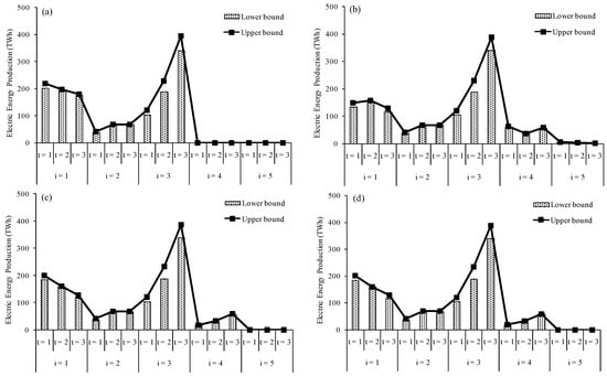
Figure 1.
Electric energy productions under each scenario (a) LU-LT scenario; (b) LU-HT scenario; (c) HU-LT scenario; (d) HU-HT scenario.
In the LU-HT scenario, the amount of electricity generated by coal-fired power has on the rise after a sharp decline. But in the third planning period, the amount has declined again. Wind power still has been the primary source of regional electric power. However, solar power and biomass power have acted the supplemental function. In HU-LT scenario and HU-HT scenario, the same result of power generation has been obtained, that means with a high utilization ratio, the change of emission reduction target would have no direct impact on the structure of regional electric power system. Specifically, the amount of electricity generated by coal-fired power will continue to decline with a rate between LU-LT scenario and LU-HT scenario. Meanwhile, the amount of electricity generated by solar power will increase gradually, and reach 18.22, 32.79 and 59.02 TWh in each planning period. The amount of electricity generated by biomass power will be zero and remain consistent.
As for the same planning period in different scenario, the relevant results have been shown in Figure 2. Under any circumstances, wind power will be the major way of generating electricity, and the proportion can reach at least 60 percent.
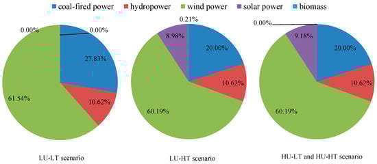
Figure 2.
Electric power structure in third planning period.
The proportion of coal-fired power will decline to about 20 percent. However, coal-fired power will remain the second energy source. Meanwhile, the results shown that biomass power would be almost zero and remain consistent, that mean biomass power compared with other technologies had a gap in economic efficiency. Solar power will maintain zero in the LU-HT scenario. Even in the best of circumstances, the proportion will be less than 10%.
Figure 3 and Figure 4 displays the total system cost and the percent of risk cost in different planning period. In different scenario, the total system cost from highest to lowest will be HU-HT scenario, LU-HT scenario, HU-LT scenario and LU-LT scenario. Meanwhile, with a same emission reduction target, the result will be very close, that means unlike the utilization ratio of carbon capture technology, the emission reduction target will have more influence on total system cost. The same situation occurs in result of the percent of risk cost. For example, in the third planning period under each scenario, the total system cost will be [171.00, 215.86] × 109 $, [190.49, 245.12] × 109 $, [175.58.49, 221.79] × 109 $ and [194.77, 249.92] × 109 $, respectively. The percent of risk cost will be [6.28, 7.30], [11.27, 12.85], [5.46, 6.34] and [9.85, 11.25], respectively.
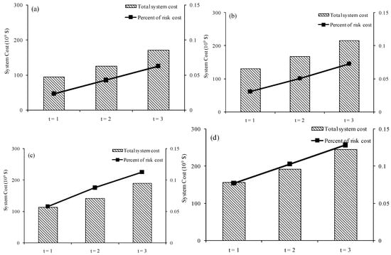
Figure 3.
Total system cost and the percent of risk cost under LU-LT scenario and LU-HT scenario. (a) Lower bound of LU-LT scenario; (b) Upper bound of LU-LT scenario; (c) Lower bound of LU-HT scenario; (d) Upper bound of LU-HT scenario.
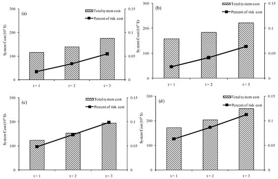
Figure 4.
Total system cost and the percent of risk cost under HU-LT scenario and HU-HT scenario. (a) Lower bound of HU-LT scenario; (b) Upper bound of HU-LT scenario; (c) Lower bound of HU-HT scenario; (d) Upper bound of HU-HT scenario.
For the same scenario, the total system cost will increase with the planning period, and this same situation exists in the results of the percent of risk cost. Further analysis on the amplitude of variation indicates that the relevant parameter of total system cost had different from the percent of risk cost. As for the interval numbers, the lower bound has a high growth rate than the upper bound.
5. Discussion
The average carbon dioxide emission and total carbon dioxide emission in different planning period is shown in Figure 5 and Figure 6. In the benchmark year, the mount of total carbon dioxide emission was 216.30 × 10⁶ tonne, and the average carbon dioxide emission was 873.50 g/kWh. In the LU-LT scenario, the mount of total carbon dioxide emission will be [181.32, 195.06] × 106 tonne, [148.37, 151.85] × 106 tonne and [114.82, 116.80] × 106 tonne, and the average carbon dioxide emission will be [524.36, 512.82], [330.04, 307.09] and [196.47, 181.69] g/kWh. In this scenario, the decline rate of total carbon dioxide emissions is lower than the average carbon dioxide emission.
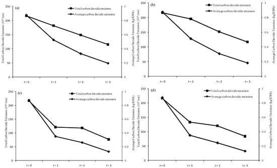
Figure 5.
Carbon dioxide emissions under LU-LT scenario and LU-HT scenario [(a) Lower bound of LU-LT scenario; (b) Upper bound of LU-LT scenario; (c) Lower bound of LU-HT scenario; (d) Upper bound of LU-HT scenario].
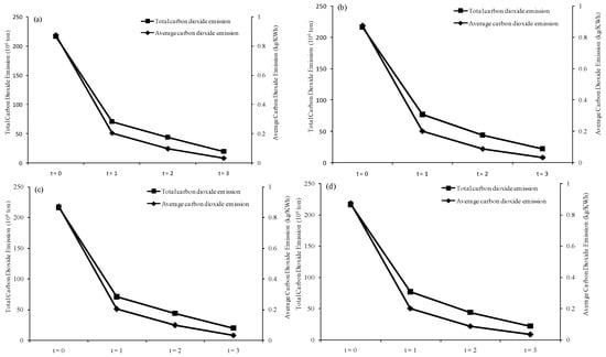
Figure 6.
Carbon dioxide emissions under HU-LT scenario and HU-HT scenario (a) Lower bound of HU-LT scenario; (b) Upper bound of HU-LT scenario; (c) Lower bound of HU-HT scenario; (d) Upper bound of HU-HT scenario].
In the LU-HT scenario, the mount of total carbon dioxide emission will be [120.82, 132.90] × 106 tonne, [117.80, 120.60] × 106 tonne and [76.29, 83.92] × 106 tonne, and the average carbon dioxide emission will be [349.40, 349.40], [262.05, 243.82] and [130.55, 130.55] g/kWh. In the second planning period, the mount of total carbon dioxide emission is close to the previous planning period, and it has clearly indicated that the decline of average carbon dioxide emission is not syncing up with the total carbon dioxide emission. In the remaining two scenarios, the average carbon dioxide emission and total carbon dioxide emission have to be down dramatically. The result is [70.74, 76.63] × 106 tonne, [43.69, 43.69] × 106 tonne, [19.78, 21.76] × 106 tonne, [204.57, 201.46], [91.19, 88.36] and [33.86, 33.86] g/kWh.
Comparing different scenarios, the results are quite different. The maximum value of the total carbon dioxide emissions has more than tripled compared to the minimum. That indicates the utilization ratio of carbon capture technology and the target for carbon emissions reduction will have a significant impact on regional development planning. Of the two factors, the utilization ratio of carbon capture technology will play a larger role in carbon emission reduction. That also means the decision maker should focus more energy on the spread of carbon capture technology. As technology matures and cost reduction, the carbon emissions reduction targets will be met.
The quantity of the discharged air pollutants during the different period is shown in Figure 7. In different scenario, the quantity of the discharged air pollutants will reduce. Among these scenarios, the LU-LT scenario and LU-HT scenario will have the worst and best air quality respectively. Taking sulfur dioxide as an example, the quantity will be [150.34, 161.73] × 103 tonne, [107.00, 109.51] × 103 tonne, [65.08, 66.21] × 103 tonne in the LU-LT scenario. But in the LU-HT scenario, the quantity will be only 70 percent to 80 percent of the worst situation. The results indicate that higher target for carbon emissions reduction will reduce the electric power coming from coal-fired power plants and promote the development of renewable energy. Furthermore, the quantity of discharged air pollutants will decrease.
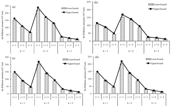
Figure 7.
Air pollutants discharged during the different period (a) LU-LT scenario; (b) LU-HT scenario; (c) HU-LT scenario; (d) HU-HT scenario.
6. Conclusions
An interval fuzzy programming with risk measure model was applied to regional electric power system management in Xinjiang, China. Interval values, fuzzy programming and risk measure were incorporated within a general optimization framework. Tradeoffs between production cost, risk cost, structure of electric power system, air pollutant emission, utilization of new technologies and carbon emission reduction were analyzed. Different scenarios have been tested to verify the suitability and effectiveness of the method. The developed model could help decision makers formulate and adjust regional electric development plans under various environmental, economic, energy and technical considerations. Specifically, some conclusions were obtained as follows. It was concluded that setting of emissions targets would relieve the pressure of climate change and reduce emissions of air pollutants. The utilization of carbon capture technology could also significantly reduce the carbon emission, even with lower carbon emissions reduction target, and decision makers should put much more effort into promoting and improving carbon capture technology. In order to reduce carbon dioxide, wind power and hydropower would be the best choice. Coal-fired power would be the suboptimal choice, and solar power would play a complementary role because of being limited by the high cost. There were obvious disadvantages in biomass power, which included air pollutant emission and high price of biomass fuel.
The interval fuzzy programming with risk measure model has been proved to be effective in the case study. However, the present study has some limitations. Such a method will encounter difficulties when the model’s coefficients are associated with more complex uncertainties. The following study could focus on several aspects. First, the emission of greenhouse gases should not only be restricted in burning process, and the related emission from energy resources exploitation and transportation would be considered; more environmental pollution from power generation and the secondary pollution from the view of life-cycle assessment (e.g., pollutant release in photovoltaic) should be taken into consideration [31]. Second, during model development, the breakthrough of technologies, which included power generation technologies and carbon capture technology, should be considered. Third, a more refined model, including nuclear power, offshore wind power, refuse-burning power and so on, will be established in the future study.
Author Contributions
Y.X. and Z.F. designed the manuscript; Y.X., Z.F., and G.H. drafted the manuscript; D.X., W.L., and H.W. collected the data and revised the manuscript; Y.X., Z.F., and G.H. checked the content and revised the manuscript. All authors made contributions to the study and the writing of the manuscript.
Funding
This research was supported by the National Natural Science Foundation of China (51609003 and 71603016), the Fundamental Research Funds for the Central Universities (FRF-BD-18-015A), and the China Postdoctoral Science Foundation funded project (Grand No. 2015M580046 and Grand No. 2015M580034).
Conflicts of Interest
The authors declare no conflict of interest.
References
- Yan, J.Y.; Zheng, Z.N. Carbon Capture, Utilization and Storage (CCUS). Appl. Energy 2019, 235, 1289–1299. [Google Scholar] [CrossRef]
- Padron, E.; Melian, G.; Marrero, R.; Nolasco, D.; Barrancos, J.; Padilla, G.; Hernandez, P.A.; Perez, N.M. Changes in the diffuse CO2 emission and relation to seismic activity in and around El Hierro, Canary Islands. Pure Appl. Geophys. 2008, 165, 95–114. [Google Scholar] [CrossRef]
- Girault, F.; Bollinger, L.; Bhattarai, M.; Koirala, B.P.; France-Lanord, C.; Rajaure, S.; Gaillardet, J.; Fort, M.; Sapkota, S.N.; Perrier, F. Large-scale organization of carbon dioxide discharge in the Nepal Himalayas. Geophys. Res. Lett. 2014, 41, 6358–6366. [Google Scholar] [CrossRef]
- Carpinteri, A.; Borla, O. Nano-scale fracture phenomena and terahertz pressure waves as the fundamental reasons for geochemical evolution. Strength Fract. Complex. 2018, 11, 149–168. [Google Scholar] [CrossRef]
- Carpinteri, A.; Niccolini, G. Correlation between the Fluctuations in Worldwide Seismicity and in Atmospheric Carbon Pollution. Science 2019, 1, 2. [Google Scholar] [CrossRef]
- Liu, W.; Lund, H.; Mathiesen, B.V.; Zhang, X.L. Potential of renewable energy systems in China. Appl. Energy 2011, 88, 518–525. [Google Scholar] [CrossRef]
- Chu, S.; Majumdar, A. Opportunities and challenges for a sustainable energy future. Nature 2012, 488, 294–303. [Google Scholar] [CrossRef]
- Arasto, A.; Tsupari, E.; Kärki, J.; Sihvonen, M.; Lilja, J. Costs and potential of carbon capture and storage at an integrated steel mill. Energy Procedia 2013, 37, 7117–7124. [Google Scholar] [CrossRef]
- Rackley, S.A.; Rackley, S.A. Overview of carbon capture and storage. Carbon Capture Storage 2010, 41, 19–28. [Google Scholar]
- Cormos, C.C. Integrated assessment of IGCC power generation technology with carbon capture and storage (CCS). Energy 2012, 42, 434–445. [Google Scholar] [CrossRef]
- Rubin, E.S.; Davison, J.E.; Herzog, H.J. The cost of CO2 capture and storage. Int. J. Greenh. Gas Control 2015, 40, 378–400. [Google Scholar] [CrossRef]
- Delucchi, M.A.; Jacobson, M.Z. Providing all global energy with wind, water, and solar power, Part II: Reliability, system and transmission costs, and policies. Energy Policy 2011, 39, 1170–1190. [Google Scholar] [CrossRef]
- Jacobson, M.Z.; Delucchi, M.A. Providing all global energy with wind, water, and solar power, Part I: Technologies, energy resources, quantities and areas of infrastructure, and materials. Energy Policy 2011, 39, 1154–1169. [Google Scholar] [CrossRef]
- Wu, C.B.; Huang, G.H.; Li, W.; Xie, Y.L.; Xu, Y. Multistage stochastic inexact chance-constraint programming for an integrated biomass-municipal solid waste power supply management under uncertainty. Renew. Sustain. Energy Rev. 2015, 41, 1244–1254. [Google Scholar] [CrossRef]
- Calvillo, C.; Sanchez-Miralles, A.; Villar, J. Energy management and planning in smart cities. Renew. Sustain. Energy Rev. 2016, 55, 273–287. [Google Scholar] [CrossRef]
- Dellano-Paz, F.; Calvo-Silvosa, A.; Antelo, S.I.; Soares, I. Energy planning and modern portfolio theory: A review. Renew. Sustain. Energy Rev. 2017, 77, 636–651. [Google Scholar] [CrossRef]
- Prebeg, P.; Gasparovic, G.; Krajacic, G.; Duic, N. Long-term energy planning of Croatian power system using multi-objective optimization with focus on renewable energy and integration of electric vehicles. Appl. Energy 2016, 184, 1493–1507. [Google Scholar] [CrossRef]
- Wolfram, P.; Wiedmann, T.; Diesendorf, M. Carbon footprint scenarios for renewable electricity in Australia. J. Clean. Prod. 2016, 124, 236–245. [Google Scholar] [CrossRef]
- Al-Hamamre, Z.; Saidan, M.; Hararah, M.; Rawajfeh, K.; Alkhasawneh, H.E.; Al-Shannag, M. Wastes and biomass materials as sustainable-renewable energy resources for Jordan. Renew. Sustain. Energy Rev. 2017, 67, 295–314. [Google Scholar] [CrossRef]
- Parkinson, S.C.; Djilali, N. Long-term energy planning with uncertain environmental performance metrics. Appl. Energy 2015, 147, 402–412. [Google Scholar] [CrossRef]
- Ji, L.; Huang, G.H.; Huang, L.C.; Xie, Y.L.; Niu, D.X. Inexact stochastic risk-aversion optimal day-ahead dispatch model for electricity system management with wind power under uncertainty. Energy 2016, 109, 920–932. [Google Scholar] [CrossRef]
- Niet, T.; Lyseng, B.; English, J.; Keller, V.; Palmer-Wilson, K.; Moazzen, I.; Rowe, A. Hedging the risk of increased emissions in long term energy planning. Energy Strategy Rev. 2017, 16, 1–2. [Google Scholar] [CrossRef]
- Büyüközkan, G.; Güleryüz, S. Evaluation of renewable energy resources in turkey using an integrated mcdm approach with linguistic interval fuzzy preference relations. Energy 2017, 123, 149–163. [Google Scholar] [CrossRef]
- Osuna-Gómez, R.; Chalco-Cano, Y.; Hernández-Jiménez, B.; Aguirre-Cipe, I. Optimality conditions for fuzzy constrained programming problems. Fuzzy Sets Syst. 2018. [Google Scholar] [CrossRef]
- Messner, S.; Golodnikov, A.; Gritsevskii, A. A stochastic version of the dynamic linear programming model MESSAGE III. Energy 1996, 21, 775–784. [Google Scholar] [CrossRef]
- Krey, V.; Riahi, K. Risk hedging strategies under energy system and climate policy uncertainties. Int. Ser. Oper. Res. Manag. Sci. 2013, 199, 435–474. [Google Scholar] [CrossRef]
- Wang, C.J.; Wang, F.; Zhang, X.L.; Zhang, H.G. Influencing mechanism of energy-related carbon emissions in Xinjiang based on the input-output and structural decomposition analysis. J. Geogr. Sci. 2017, 27, 365–384. [Google Scholar] [CrossRef]
- Xiao, R. On the role of Xinjiang in guranteeing China’s energy security. Financ. Econ. Xinjiang 2013, 1, 52–56. [Google Scholar]
- Duan, J.; Wei, S.; Zeng, M.; Ju, Y. The energy industry in Xinjiang, China: Potential, problems, and solutions. Power 2016, 160, 52–53. [Google Scholar]
- Mallia, E.; Lewis, G. Life cycle greenhouse gas emissions of electricity generation in the province of Ontario, Canada. Int. J. Life Cycle Assess. 2013, 18, 377–391. [Google Scholar] [CrossRef]
- Fthenakis, V.; Morris, S.; Moskowitz, P.; Morgan, D. Toxicity of cadmium telluride, copper indium diselenide, and copper gallium diselenide. Prog. Photovolt. Res. Appl. 1999, 7, 489–497. [Google Scholar] [CrossRef]
© 2019 by the authors. Licensee MDPI, Basel, Switzerland. This article is an open access article distributed under the terms and conditions of the Creative Commons Attribution (CC BY) license (http://creativecommons.org/licenses/by/4.0/).