1. Introduction
Market liberalization has taken place in many countries over the past two decades. The success of liberalization in other industries and a belief that it can be replicated in the power sector as well as a demand for unbundling the vertically integrated monopoly structures were the driving forces behind the liberalization of the power sector. Technology advancement and conceptual changes in the generation technologies and in the electric power networks have enabled a separation of what had previously been a natural monopoly. The long-term goals behind the electricity liberalization have been to entice investments, increase efficiency and further stimulate technical innovation. As a result, large integrated electric utilities have been deregulated and market schemes have started playing big roles. In any energy company’s decision making and strategy development, price forecasts have become an essential input.
Current research on electricity price forecasting can be classified in terms of the methodology applied and in terms of the planning horizon’s duration. Bearing in mind horizon duration, it is common to define short-term (STPF), medium-term (MTPF) and long-term (LTPF) price forecasting (
Figure 1) [
1]. In LTPF lead times are typically measured in years and the main objective is planning and investment profitability analysis, such as decision making for future investments of power plants, inducing locations and fuel sources. In MTPF times are typically measured in months and the focus is on balance sheet calculations, risk management, and derivatives pricing. In MTPF, often, the distributions of future prices over certain time periods are estimated rather than actual point forecasts. This is because medium-term modeling has a long history in finance, so there is a strong influence of finance solutions to this type of modeling.
Models that are applied for long and medium-term modeling can be classified as presented in
Figure 1. Simulation models are powerful in crating various future scenarios and calculating the probability of price scenarios based on risk assumption. Considering the specifics of an observed market, Equilibrium approaches build the price scenarios based on equilibrium models. Production cost models simulate the operation of generating units to satisfy the system demand at a minimum cost based on merit order list. Fundamental methods define price movements by modeling the impact of important economic and physical factors on the electricity price.
In addition to monthly or annual time horizons, short-term planning is important for generators, utilities, and market participants for the operational implementation of long- and medium-term plans. In an auction-type environment, when bidding for spot electricity, market participants are requested to place their bids in terms of prices and quantities. Orders are accepted in order of increasing or decreasing prices until total demand and supply is met. A generator that can accurate forecast spot prices can adjust its own production schedule accordingly and hence maximize its profits. Day-ahead spot market typically consists of 24 hourly (or 96 of 15-minute) auctions that take place simultaneously one day in advance. STPF with lead times from a few hours to a few days are of prime importance in day-to-day market operations. In power systems with complex market structures, generation companies and other market players can sell or buy electricity either directly through bilateral contracts or from a centralized power pool. This research describes a pool-based energy market as it is the most common type of market, where the producers and consumers submit their bids that consist of a set of quantities with prices. Using a market clearing algorithm, the market operator then determines the prices for the next day Day ahead price forecasting is a most valuable tool for all the market participants as it defines decision making for the operation of a power plant and the portfolio optimization on the spot market. Price series have complex features such as non-stationarity, nonlinearity, and high volatility, which make forecasting very challenging. This is because of the basic characteristics of electricity, which is its non-storable nature, the requirement of maintaining a continuous balance between supply and demand and rigid nature of demand over a short time period. Therefore, a decent price prediction model should be able to capture the complex behavior associated with price series. Models used in STPF can be divided into three categories: statistical models, models based on artificial intelligence, and hybrid models (
Figure 1).
2. Short-Term Forecasting Methodologies
Taking into account the importance and complexity of short-term price forecasting various methods for price forecasting have been introduced by researchers. Three widely used approaches are time series models, artificial neural networks (ANN) and hybrid methods.
2.1. Time Series Models
Auto-regressive integrated moving average (ARIMA) and non-stationary time series models such as generalized auto-regressive conditional heteroskedastic (GARCH) and dynamic regression (DR) are mostly used stationary models for time series forecasting.
In [
2] Swider and Weber proposed extended ARMA models for estimating price developments on day-ahead electricity markets. ARMA model in combination with a GARCH was demonstrated for a European Energy Exchange (EEX) market price forecast from January 2002 to January 2004. In [
3] Nogales et al. used dynamic regression (DR) and transfer function (TF) models for the prediction of prices on the Spanish (Operador del Mercado Ibeico de Energia) OMEL market from January to November 2000 and the California market from January to April 2000. In [
4] Contreras et al. used the ARIMA method on Spanish OMEL market for the prediction of short-term electricity prices from January 2000 to November 2000, and on the California market from January 2000 to April 2000. In [
5] Bordignon et al. used autoregressive moving average parts with linear regression (LR), exogenous variables (ARMAX), time-varying parameter regression (TVR), and Markov regime switching model (MS) methods in prediction price on the United Kingdom Power Exchange (UKPX) market during from April 2005 to September 2006.
2.2. Artificial Neural Network Methods
Electricity price is not a linear function of its input parameters and this may create a significant problem for the time series techniques to accurately capture the dynamic performance of the price signal as most time series models are based on linear predictors. To overcome this problem, models based on neural networks (NN) and fuzzy neural networks (FNN) have been introduced to electricity price forecasting. In [
6] the authors presented models based on three different neural networks for the day-ahead price estimation, these included the feed-forward (FFNN), cascade-forward (CFNN), and generalized-regression (GRNN) neural networks. Models were tested on the Spanish market (OMEL) data from 2002 and the Pennsylvania New Jersey Maryland market (PJM) data from 2010. In [
7] Amjady used a fuzzy neural network (FNN) for the forecast of the electricity prices on the OMEL market from February to November 2002. In [
8] the authors introduced an innovative method based on self-organizing map neural network (SOM) and support vector machine (SVM) models to predict the day-ahead electricity prices and tested it on the PJM market data from August 2002. In [
9] a novel approach was presented using a sensitivity analysis of similar days (SD) parameters to increase the accuracy of the results obtained by artificial neural networks (ANN). This method was tested on the PJM market from January to December 2006.
2.3. Hybrid Methods
Hybrid methods combine both linear and nonlinear modeling strategies. To improve the forecasts, hybrid methods use each model’s specific features to detect different patterns in the data and conjointly yield a more accurate result. In [
10] the authors present a hybrid method to predict the day-ahead prices based on radial-basis-function neural networks (RBFN), wavelet transform (WT), and auto-regressive integrated moving average (ARIMA) models. The results are presented on the OMEL market data from 2002. In [
11] the authors propose a hybrid method based on WT, ARIMA and least squares support vector machine (LSSVM) optimized by particle swarm optimization (PSO). Their method is tested on the data from New South Wales (NSW) of Australian national electricity market from 2007 to 2008. In [
12] the authors suggest a hybrid method based on the combination of PSO and adaptive-network fuzzy inference system. Like several of the previously mentioned methods, this method is also tested on the OMEL market data from 2002.
There is no precise answer to which of these models is the best and which will give the best results. Phatchakorn Areekul et al. [
13] presented a comparison of ARIMA, ANN, and a proposed hybrid method that combines ARIMA and ANN using data from the Australian national electricity market, New South Wales from January to November 2006. Forecasting errors were in the range of 10.46% to 16.07% for ARIMA, 10.04% to 15.63% for ANN, and 9.99% to 15.63% for the hybrid method. These results indicate that sophisticated, fine-tuned representatives of both groups might compete on equal terms if they were compared in a comprehensive and thorough study.
2.4. State of the Art: Quantitative Analysis
As part of this research, a quantitative analysis of scientific articles from the field of forecasting of electricity prices was carried out. In order to make an analysis, the following query was used for the search on the Web of Science portal:
TS = ((“forecasting” OR “predicting”) AND (“electricity spot price” OR “electricity day-ahead price” OR “electricity price” OR “power price”)).
Figure 2 shows an overview of the search results of the methods listed in the keyword list.
From this simple analysis, it is evident that the number of articles in the field of electricity price forecasting has increased over the years. In addition, it can be concluded that statistical methods and neural networks are constantly being applied, and it is also apparent that the number of articles referring to hybrid methods has increased in recent years.
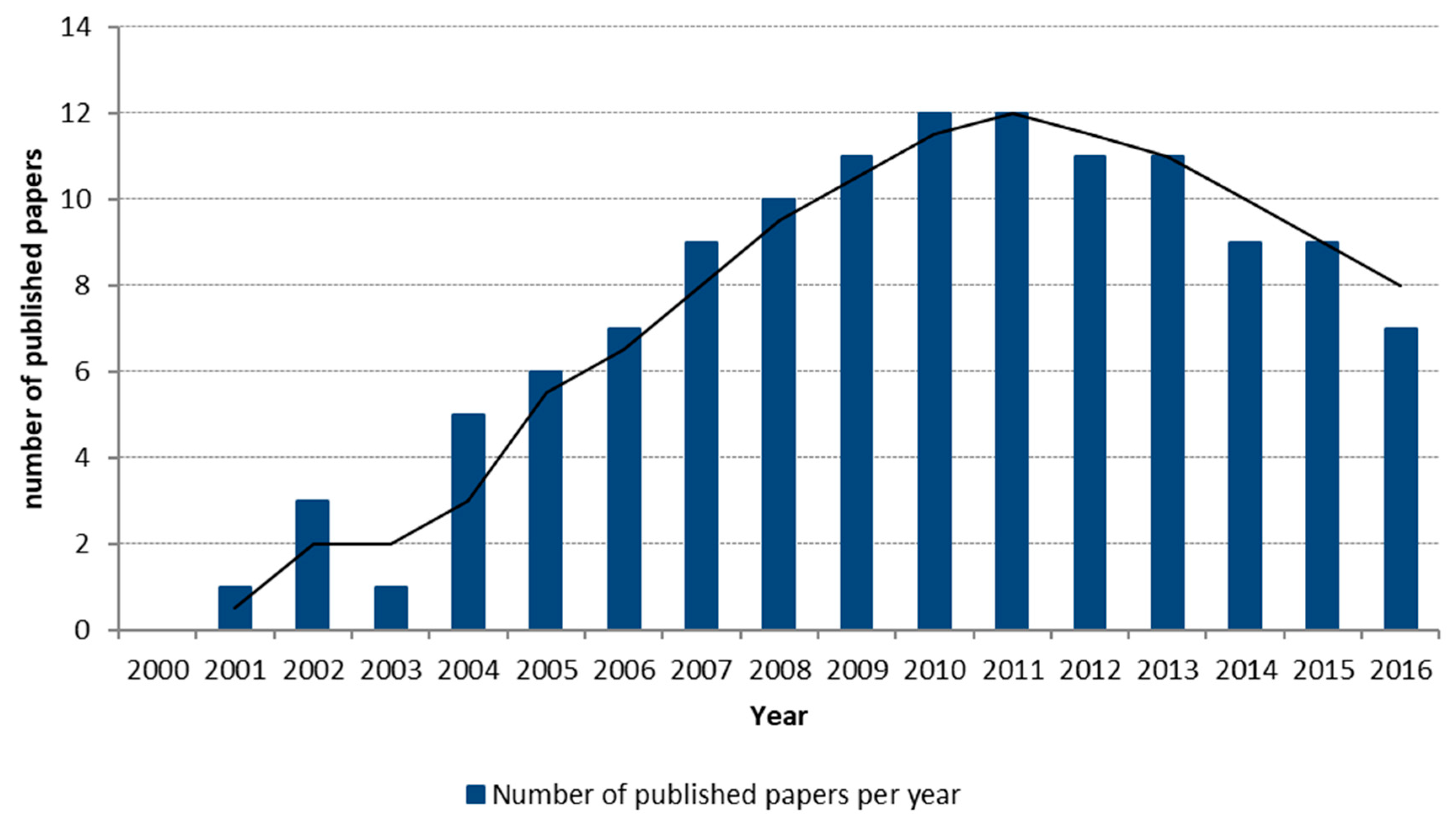
This simple quantitative analysis was a motivation for a more complex analysis that analyzed in detail scientific articles on electricity price forecasting published in IEEE Xplore and Science Direct databases. The analysis was made on a sample of over 100 articles published in the period from 1999 to 2017. Part of the research was presented in the authors’ previous article [
1] and for this research an additional analysis of the articles was made using the same methodology (
Figure 3). The analysis observed the following characteristics:
Forecasting time horizon
Method used for electricity price forecasting
Input parameters used for electricity price forecasting
Market on which method was tested
A range of historical data used for forecasting
Tools used for forecasting
Price forecasting error
A similar analysis of published articles was made by Pandey and Upadhyay [
14], the main feature of their analysis was the categorization of research papers according to the price forecasting methods classification presented in
Figure 1. An extensive analysis of state of the art was made by Weron [
15], where each of the price forecasting models was explained in detail with all the typical applications in previously published works.
The state of the art analysis presented partly in this article and in the previously published article [
1] focuses on practical aspects of the application of forecasting methods such as the number of input parameters, forecasting error, and the market on which the model was tested. Based on the collected data from [
1] and [
14,
15,
16,
17], a number of statistical indicators were obtained that could provide certain guidelines for making conclusions related to the problem of predicting electricity prices.
Classification of methods used for electricity price forecasting is made according to
Figure 1 and the result of this classification is shown in
Figure 4.
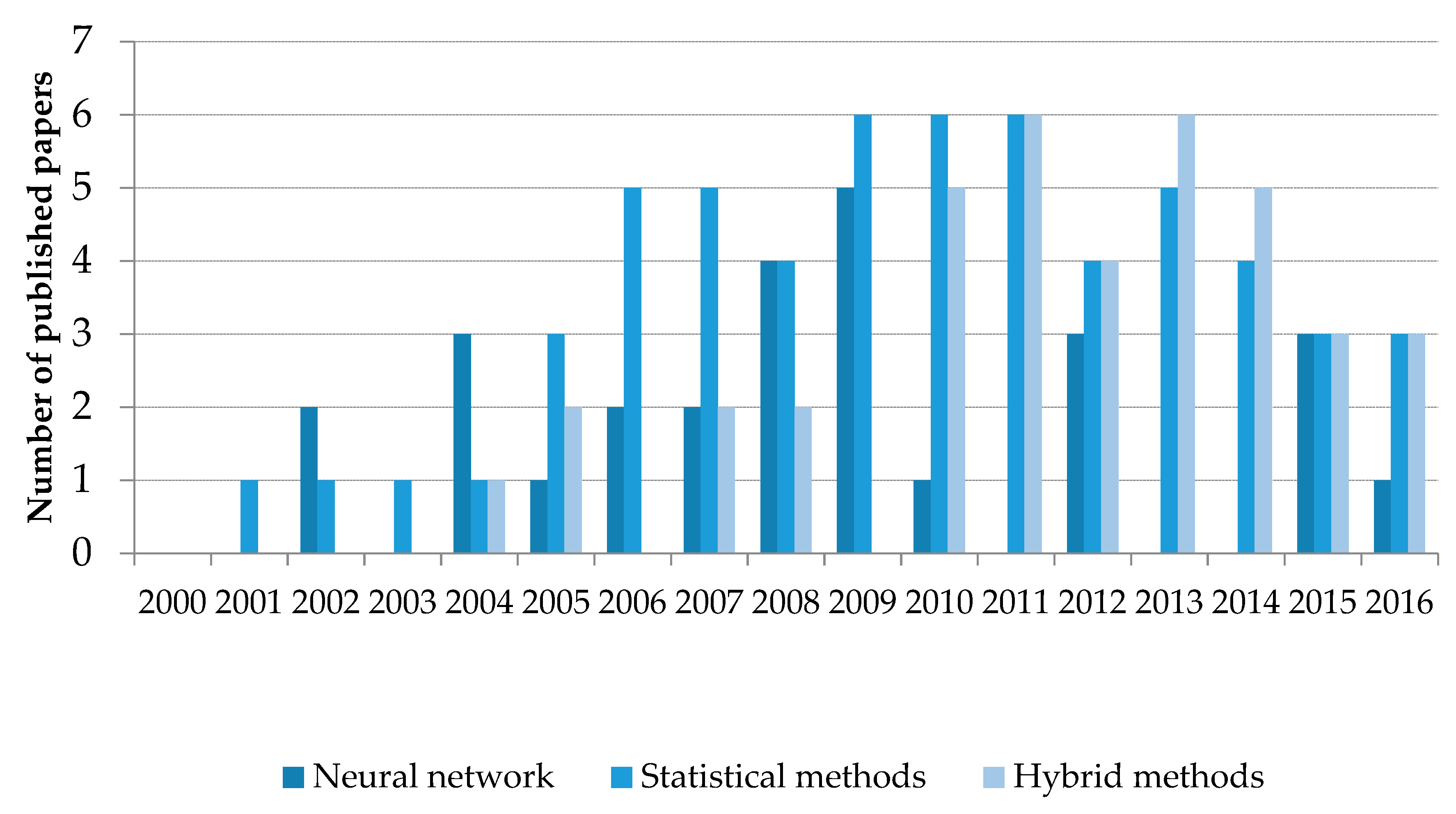
In the analyzed sample of published articles, statistical methods are the most frequently used tool for predicting prices (
Figure 4). When this distribution is observed over a time horizon (
Figure 5), statistical methods are constantly represented in price prediction, neural networks have been used more before 2010, and since 2010 hybrid methods have become an increasingly common tool for predicting electricity prices.
An interesting indicator is the number of input parameters used by researchers to test the proposed models for predicting electricity prices (
Figure 6).
The most common input parameter is historical prices, the second most common parameter is time parameters, such as date and type of day, and the third most common parameter is electricity consumption [
18]. The range of input parameters in articles that are using more than three input parameters is diverse: structure of engaged power plants in the power system, weather forecasts, production from renewable energy sources, cross-border exchange of electricity, intraday market, smart grid, etc., [
19,
20].
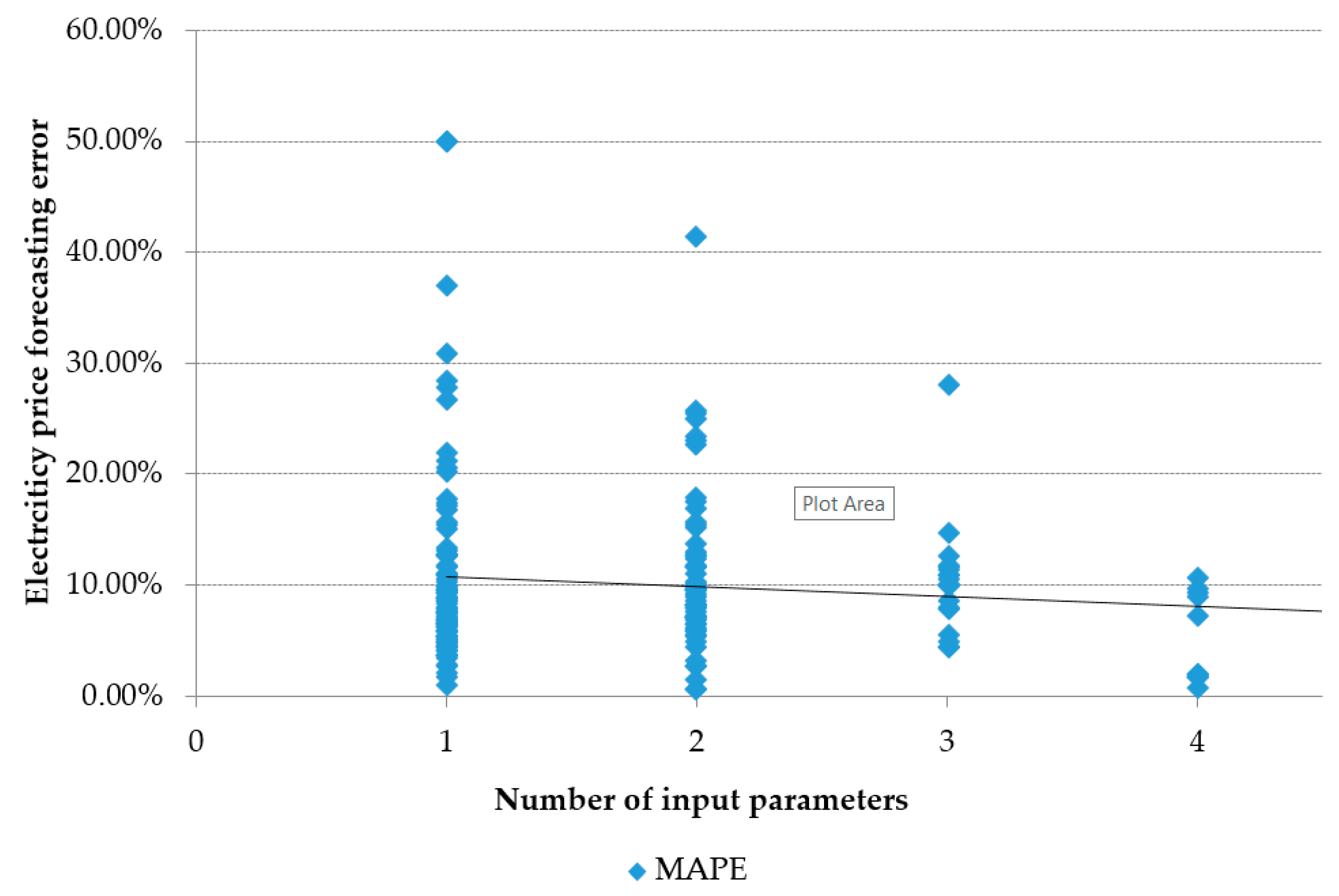
A forecasting error is a relative term because not all articles use the same accuracy indicators. Since Mean Average Percentage Error (MAPE) is used in most cases, articles that used this indicator were considered in this analysis. The correlation between MAPE and the number of input parameters used for forecasting is shown in
Figure 7. With more input parameters a smaller range of forecasting errors can be expected. In most of the reviewed papers, input parameters included flexible production based on the merit order list. However, a higher share of renewable sources production input parameters with high uncertainty may increase forecasting error. In that respect, new approach based on the correlation between spot prices and residual load (difference between consumption and non-flexible production) has been advocated in Reference [
21]. Based on this new approach, it is noted that, while using a large number of input variables, it is important to carry out a sensitivity analysis for input variables and use only those that have a significant influence on electricity prices.
It can be concluded that with more input parameters more accurate results can be achieved. However, sometimes in scientific papers theoretical models with a high accuracy of price forecasting are described, which are not realistically applicable in practice.
This review of the state of the art analyzed a large number of articles on the topic of electricity price forecasting, and the analysis results led to the following conclusions:
The problem of predicting electricity prices is a current topic of research in scientific circles
Only a small number of articles use a large number of input parameters, which is why the author believes that this is the area where scientific potential should be directed, given the rapid development of the electricity market, increasing market transparency, and the transparency of the operation of electric power systems
Hybrid methods are becoming more and more popular, because they are an excellent tool for processing and analyzing large amounts of data, and for preparing inputs for some of the existing methods for predicting electricity prices
3. Hybrid Iterative Reactive Adaptive (HIRA) Price Forecasting Method
As discussed in the previous section, existing price forecasting methods have several limitations. Some models are applicable only in certain markets due to the degree of market development and available market data. Some models are only limited to linear price modeling while prices often form a nonlinear function. There are models which give less accurate price forecasts in conditions of high price volatility and are not responsive to various changes of conditions in the market. Finally, many models take only a small set of input parameters as a basis for price calculation, while it is notable that with the use of a larger number of input parameters and input datasets, the forecasting error (MAPE) decreases. To address these limitations, a new Hybrid Iterative Reactive Adaptive (HIRA) price forecasting model is proposed:
The HIRA method is illustrated with the flow chart in
Figure 8 and is divided into two phases:
analysis phase—the phase of analysis of power system for which the price is forecasted and analysis of its neighboring power systems, in order to determine the parameters that have influence on forming of the prices in the observed market
and forecasting phase—the price forecasting based on the relevant parameters determined in the analysis phase.
In the phase of the analysis of the power system, by identifying the key parameters that affect the price of electricity on a given market, the HIRA model adapts to the specifics of the market on which it is used, i.e., the model is adaptable to the characteristics of the observed market.
The price forecasting phase uses a hybrid method that combines two methods for predicting prices; a statistical method of similar day and neural networks. Using neural networks this model responds to the challenge of a large number of available input parameters and data for forecasting prices. The forecasting phase is if possible and as needed, carried out in several iterations before auctions in the spot market of the electricity market, with the aim of efficiently managing the market and the production portfolios. In each iteration new and updated data is used for forecasting, and thereby the HIRA model reacts to changes in the market and/or in the power system that can affect price formation. In this way, the estimated price from each iteration ensures timely decision-making and management of price risks, which makes the HIRA model reactive to changes in the market.
The number of iterations, i.e., the time intervals when price forecasts will be calculated, is determined depending on the development of the electricity market for which the prices are forecasted. For example, input data that affect price formation are more accessible and more volatile in developed markets, which requires more frequent updating of price forecasts or shorter intervals of iterations.
3.1. Power System Analysis
In power system analysis phase, the market is analyzed as well as the surrounding markets. The result of the analysis is a set of internal and external parameters that influence the formation of electricity prices in the observed market.
Internal parameters describe the market for which the price is forecasted. Internal input data include basic data on the functioning of the observed power system, which can be classified as data on electricity consumption, electricity production, and the cross-border exchange of electricity (import/export).
External factors can also have an influence on electricity prices. An external factor could be the behavior of electricity market traders who are making a profit by arbitration procedures in several related markets, therefore, their speculative actions can affect the formation of electricity prices. Another example of an external influence is a high production of electricity from hydro power plants or other renewable sources such as wind in the neighboring power system. During the hours when the wind production is high, the incoming flow of energy from the neighboring electricity system increases, which can lead to a decrease of prices in the observed market. External parameters are defined by collecting external input data describing the fundamental parameters of neighboring markets, cross-border energy flow, electricity prices, data from organized markets where continuous electricity trading takes place, as well as other parameters that can affect the perception of traders when trading on a spot market.
All information about European power systems are available on the ENTSO Transparency Platform. This data represents the internal input parameters data and serves as the basis for setting up the HIRA price prediction model. External input data for the model are also available on the ENTSO Transparency Platform, as well as on the Joint Allocation Office [
22] website, also there are data from the platforms for continuous trading of standard electricity products (TFS [
23]), and data from the REMIT portal.
Input data for the HIRA model were structured as 24 datasets for each hour in a day. Dataset timestamp contains data about time (year, month, day, and hour) and type of day. Days in the input data were categorized as:
Working day (Mon–Fri)
Saturday
Sunday
Holiday
After the data were collected, it was necessary to give them a time context depending on the type of day and data availability time. Hereafter, the day for which electricity prices are forecasted is marked with d + 1, the day during which the prediction is made with d, and the previous day with d − 1. With respect to availability, electricity price data are available at the hourly level immediately upon the realization, while the data on planned production and consumption are available on d − 1 and d for d + 1. Accordingly, at any given moment there are three types of available data used for price forecasting:
Historical pricing data for the period d − 1 and older
Data for day d at hour h consisting of data on price realization for the period 00:00–(h − 1: 00), and planning data for h − 24
Planning data for d + 1 available on day d
Due to the time component of the input data described above, the HIRA method is iterative, that is, price forecasting is carried out on multiple occasions depending on the data availability, which makes price forecasts reactive to changes in the real-time electricity market, a feature that is not present in existing methods for electricity price forecasting.
3.2. Electricity Price Forecasting
Since not all input data is always available as explained above, the HIRA method for price prediction is designed in a way that it is iterative and time-dependent on data availability. When forecasting prices, the following forecasting methods are used depending on the number of available input parameters at the moment of calculating:
For up to 3 parameters (historical price data, electricity consumption, time context) similar day method is used;
For more than 3 parameters a hybrid method that combines similar days and neural networks is used.
This procedure is repeated several times according to the determined number of intervals when the prices will be forecasted.
In the proposed HIRA model for forecasting electricity prices, the hybrid prediction model consists of a linear price component and a component calculated with neural networks:
where:
3.2.1. Linear Electricity Price Component Calculated with Similar Day Method
As shown in the HIRA method flowchart in
Figure 8, in case of a small number of input parameters a similar day method is used for electricity price forecast calculation. From previously published articles [
1,
9], it can be concluded that electricity prices correlate best with the electricity consumption parameter, therefore, when using a similar day method, the consumption of electricity is used as the input parameter for the model. Electricity consumption is also the parameter that has been the most frequent topic of scientific papers for years, and with the development of methods and techniques, the prediction of consumption has been brought to a very high accuracy [
24].
The HIRA method proposes the process of determining a set of similar days using the actual historical data. Depending on the seasonality of the data being analyzed, different markets will have different values of the historical range of days
D, consequently by analyzing actual data the model is adaptable and applicable to the respective market on which it is used for price forecasting. First, it is necessary to take a set of historical data for at least for two years. With electricity consumption as the input parameter, a set of similar days
SSD(
T) is determined as a range of electricity consumption historical data with the following criteria:
with a condition
where
The historical range of days
D for a specific market is determined empirically; several price forecasts are calculated using a similar day method by varying a historical range
D. The historical range
D that resulted in the smallest forecasting error measured with MAPE is to be taken as a historical range for forecasting.
The result is SSD(T) a subset of data containing historical data on electricity prices with similar electricity consumption. This eliminates situations when electricity price forecasts may be affected by historical data of some extreme circumstances which occurred, such as extreme high or low temperatures, sports events, etc. Criteria for determining a subset of historical data with similar days is average deviation of consumption within the same category of similar days.
The price forecast for each individual hour in the linear component
L(
T)
h of the HIRA model based on the
SSD(
T) historical data set is determined on the basis of average hourly price deviation of each individual hour:
where:
3.2.2. Neural Network Component
If more than three input parameters (internal or external) are available, a hybrid model is used for calculating prices forecast. The component of forecasted price that is calculated with neural network in the HIRA model represents the price oscillation due to new input parameters. There are a large number of scientific papers where neural networks are used, however, in cases of high price volatility the results are not satisfying [
25], therefore, in the HIRA model neural networks are used only to calculate the deviation of the predicted price caused by changes in input data. Maryniak and Weron conclude that electricity prices are mostly affected by traders’ behaviors rather than by the fundamental characteristics of an electric power system [
26], which is another reason for applying a model that combines a similar day and neural network method. That way, if there is a certain price pattern, it might be found with at least one of the methods applied and thus reduce the price forecasting error.
Before using a hybrid model, it is important to determine which input parameters are relevant. This step is necessary in order to reduce a set of input data and to achieve better neural network processing performances. Determining of the influence of input parameters on the forecast of electricity price is also carried out with neural networks.
The proposed HIRA method uses neural networks to analyze the sensitivity of the forecasted price to the input parameters. A subset of historical data
S(
T)
h from the existing
SSD(
T) data set serves as test data set for training the neural network. Each of the input parameters, internal and external, are tested separately. Sensitivity analysis is carried out for each input parameter individually by fixing the value of other input parameters and using the neural network to calculate the price forecast. Depending on the number of test cases (
i) of price forecasting, Δ
i is calculated as the difference between the maximum and minimum value of the estimated price. The mean average Δ
n of all values for the selected parameter
n is calculated from all test cases as:
where:
n—total number of input parameters
i—number of test cases
maximum value of calculated price forecast in test case x for parameter n
minimum value of calculated price forecast in test case x for parameter n
average value of minimum and maximum value of forecasted price in x test cases for parameter n
The same procedure must be performed for all input parameters. Sensitivity
Oy of forecasted price to the input parameter
y is calculated as follows:
where:
y—number of input parameters (y = 1…n)
Oy—sensitivity of forecasted electricity price to the input parameter y
—average value of the difference between maximum and minimum price forecast value calculated with parameter y
Total sum of the influence of all parameters is 1, i.e., 100%. Parameters that make up 99% of the price impact are selected as the relevant parameters for predicting electricity prices in the HIRA model. This eliminates all the parameters whose impact on price prediction is not significant and which unnecessarily increase the set of data used to calculate the neural network price component. After determining which parameters are relevant, the HIRA model is fully defined and parameterized, and can be used for price forecasting.
To calculate the forecasted price component
of the HIRA model, a neural network with multi-layer perceptron (MLP) with one input, one hidden layer, and one output is used. A hybrid model takes hourly data as input. Within the existing set of similar days
SSD(
T), a new subset of data of similar hours
S(T)h is created, which consists of data from the previous iteration and new input data for the current iteration. The new input data contains hourly electricity price data that are in high correlation with the forecasted hourly price, where value 0.70 is taken as a high correlation.
where:
The neural network price component represents the difference between the predicted value calculated with the similar day method and the actual electricity price, showing how new information on the market influence electricity price and forecasting error. Therefore, to calculate the value of N(T)h, it is necessary to calculate value of L(T)h with the similar day method. The difference between L(T)h and the historical data on actual price at the hour h, form a new derived input parameter for neural network.
4. Simulation Results
The HIRA model was applied and tested on two electricity markets of different degrees of development; on German (EPEX) and Hungarian (HUPX) power exchanges. In the authors’ previous article [
27], the results of the price forecast on the EPEX Spot market for the period from December 2010 to June 2011 were presented. From the results obtained, it was concluded that the quality of price forecast results depends not only on the complexity of forecasting method but also on the characteristics of the forecasted prices. At low price volatility, the similar day method achieved acceptable results, while at higher volatility the hybrid method that combines similar day method and neural networks gave much more accurate forecasts (
Appendix A). Therefore, when testing the price forecasting method, it is very important to observe the complexity of forecasted prices which can be measured by price volatility.
This section presents the results of applying the HIRA model on the HUPX Spot market using available data for Hungarian electricity market. The prices for the period from May 1, 2017 to June 1, 2018 are forecasted on hourly resolution, with historical data from 2015 to 2018. In the analysis of the price forecasting results, an absolute forecasting error (MAPE) was measured in absolute and percentage values. It is important to show the error of forecasting through the absolute amount, because at low prices even a small forecasting error results in a very high percentage, which can lead to incorrect conclusions. In addition to forecasting errors, the results show the price volatility of the forecasted data. The price volatility measure was calculated as the standard deviation of the observed data set. In addition to forecasting results for hourly electricity prices, forecasting results for standard products on electricity market base load and peak load were presented as well.
4.1. Parameterization of HIRA Model
When optimizing the trade or production portfolio, the share of electricity to be traded at some time point is determined based on current prices and expected prices on the market in the future. On the Hungarian market it is possible to trade continuously up to the d − 3 level (three days in advance for day d) and also on the HUPX Spot market (day ahead for day d and within the day d) (
Figure 9).
On a continuous market, standard products of base load and peak load are traded. Base load energy is the delivery of the same amount of energy for 24 h in the same hourly amount, so the base load energy price is the average hourly price for all 24 h. Peak energy is the delivery of the same amount of energy in the period from 08:00 to 20:00 h in the same hourly amount, so the peak energy price is the average hourly price from 08:00 to 20:00 h.
The Hungarian power system is connected with high-voltage cross-border lines to Croatia, Serbia, Romania, Ukraine, Slovakia, and Austria. Thermal power plants comprise 90% of the installed capacity in Hungary and are a stable source of electricity, but usually with a large installed capacity per unit. Such a system is exposed to the failure of such large production units; therefore, it is very important to follow all announcements about the unavailability of certain production units on the REMIT portal. Inputs for price forecasting available data from the ENTSO Transparency Platform, the Joint Platform for Cross-Border Transmission Capacities (JAOs), and the TFS Continuous Trading Platform were used. All available data and their availability are shown in
Table 1. From the available data, the following data were used for forecasting:
Data on realized and planned electricity consumption,
Data of realized and planned renewable energy production,
Total cross-border commercial flows,
Results of daily cross-border capacity auction,
Electricity prices on neighboring power exchanges,
Data on power production in Hungary, by type (biomass, fossil fuels, run-off river hydro power plants, hydro power plants with accumulations, nuclear power plants, and others).
Balancing data was not used because it is more relevant for the intra-day market, which is not further analyzed in this article, nor is its impact on the market for the day ahead. Data on output outages and network unavailability were not used since such events are unplanned and occur in real time. Given the timeliness of the data availability presented in
Table 1, price forecasts were calculated in three intervals:
Interval d − 1
Interval d, 9:30 a.m.
Interval d, 10:30 a.m.
Once internal and external input data are defined, the HIRA model needed to be parameterized to determine the relevant set of historical data for the forecasting of electricity price. The first parameterization step was the categorization of days in week and the second was determination of the historical range D for similar day data set. The analysis was carried out using the hourly price historical data.
Table 2 shows the correlation matrix of relations between days of week calculated from the price data for the period from 2015 to 2017. High correlations starting from 0.631 are marked with red and orange colors, while very high correlations with values above 0.98 are marked with green. From this table, days of the week are divided into groups:
Working days (Monday, Tuesday, Wednesday, Thursday, Friday)
Saturday
Sundays and holidays
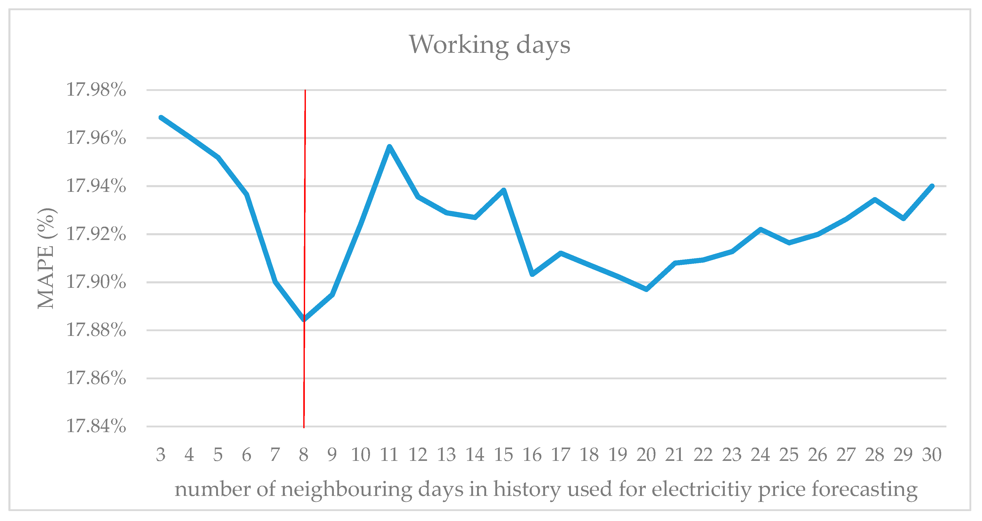
The second step of parameterization was determining the historical data range D which was used to create a set of similar days for each category of days of the week. Determination of the range D was carried out empirically, by analyzing forecasted price errors for different ranges D of historical data. Simulation was made by varying a range value D from 1 to 30 days of historical data. Test results are shown in
Figure 10,
Figure 11 and
Figure 12. The red line marks the number of historical days with the smallest forecast error.
The minimum forecasting error for working days category was achieved using a range of 9 historical days. There are 5 to 7 working days within 9 calendar days, therefore, in the historical data of 2 years, there were 25 to 35 sets of similar days to be used as a set of similar days for forecasting.
Using the same approach as for working days, the range D was calculated for Saturdays (
Figure 11); it took 21 historical days to achieve the smallest forecasting error. Within 21 days, there are three Saturdays, which means that the historical data contained 15 similar day data sets for forecasting for Saturday prices.
For Sundays and holidays, the results of the empirical analysis are shown in
Figure 12. The smallest error was achieved using 27 historical days. Within 27 days, and depending on which day is the holiday, the data set for forecasting Sunday and holidays can contain 15–20 historical days given that holidays can also be on weekdays.
For Saturdays, Sundays, and holidays, the smallest forecast errors are achieved with a significantly higher value of parameter D than for working days, but at the same time for larger values of parameter D, there is approximately a similar number of total input parameters, so it is optimal to work with 15–20 similar days in history.
With the definition of the historical data range the market analysis phase was completed and all input assumptions and necessary parameters for forecasting prices with the HIRA model were defined.
4.2. Results of Simulation in the First Iteration of the HIRA Method
In the first interval (first iteration of the HIRA method) at the time d − 1, historical electricity prices and electricity consumption forecast data are available (
Table 1). Considering a small number of input parameters, a similar day method was used with
SSD(
T)—a set of historical days obtained by parameterizing from historical data.
Table 3 shows the results of the forecasting simulation in the first iteration of the HIRA method (forecasting error for hourly prices and forecasting error for standard electricity products; base load and peak load).
Forecasting results shown in
Table 3 for base and peak energy are acceptable. Forecast error ranges between 5% and 10%, while the hourly forecasting errors are 10% to 20% which is not acceptable for application in practice.
It is interesting to observe the dependence of the price volatility and forecasting error on the example of base energy price (
Figure 13). A dotted line shows the linear interpolation of the dependence of price forecast error on the standard deviation of the price.
Figure 13 shows that the forecasting error for similar days method increases with price volatility. When applying similar days method on less volatile data, forecasting results for standard products (base load and peak load) are acceptable.
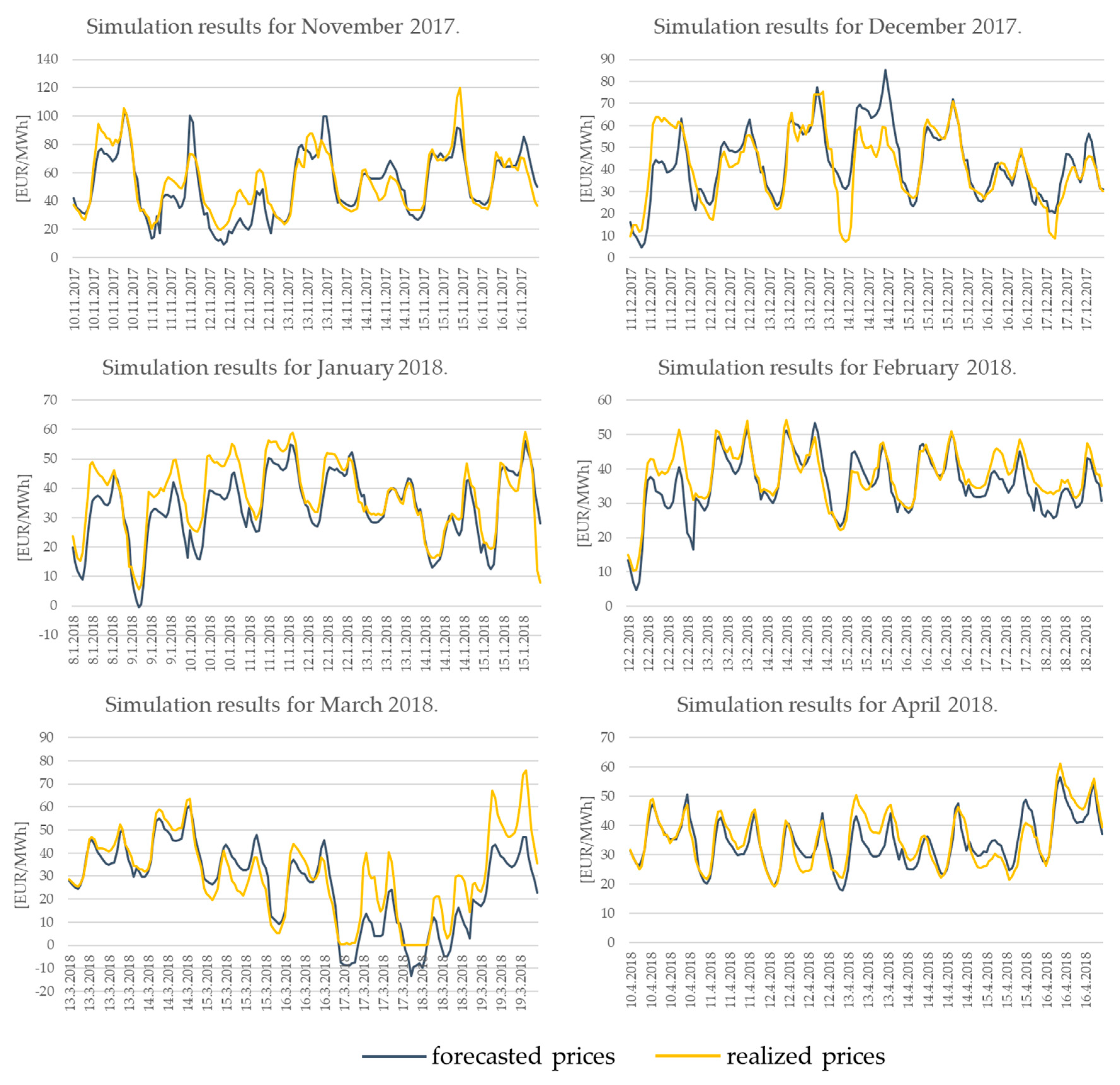
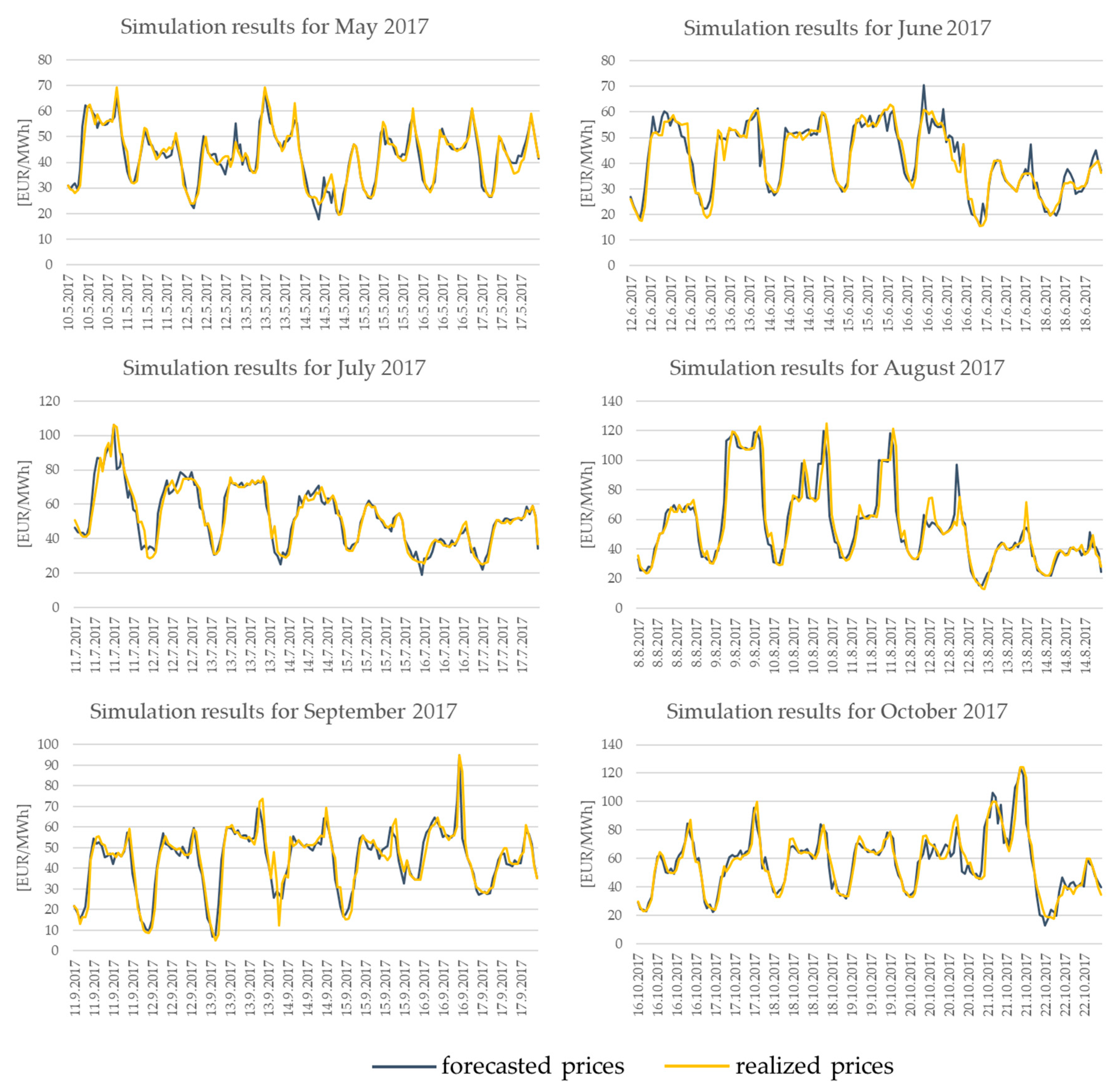
Figure 14 and
Figure 15 present the overall results of applying the HIRA model for forecasting of electricity prices in the Hungarian market in the first forecasting interval. The charts show the hourly price forecasts and realized electricity prices for the period from May 2017 to October 2017 and from November 2017 to April 2018. There are some periods where the difference between forecasted and realized prices are not negligible. Electricity prices can be very volatile on the day ahead market, which is influenced by some unexpected circumstances such as change in renewable sources production, consumption due to temperature change, power plant outage, etc. With only few input parameters available in the first iteration, these unexpected events cannot be foreseen, which causes higher forecasting error.
4.3. Results of Simulation in the Second Iteration of the HIRA Method
In the second interval (second iteration of the HIRA method) at the time of d 9:30, besides consumption data, the data on the power plant production plan and the results of auctions for cross-border capacities are available (
Table 1). Due to a larger number of available input parameters, price prediction was carried out using a hybrid method that combines the similar-day method with neural networks.
Given a large number of input parameters, a large amount of input data was collected, so it was necessary to distinguish which parameters have the highest influence on the electricity prices. In order to evaluate the importance of a particular input parameter, it was necessary to carry out a sensitivity analysis for the parameters. The results of the analysis carried out using the neural network are shown in
Appendix B. According to the proposed method for determining relevant prediction parameters, the following parameters make 99% of influence on price formation in the Hungarian market:
Renewable sources production forecast
Electricity load forecast
Price of cross-border capacity auction on Austrian-Hungarian border
Energy flow on Austrian-Hungarian border
As an input for calculating the price component obtained by neural networks, a subset of historical data was used for each hour of the day, a set of similar hours
S(
T) from a set of similar days
SSD(
T). The subset
S(
T) was created from the historical electricity price data, for each day in the similar days data set as a range (
k+ and
k−) of neighboring hours with a price correlation with forecasted hour greater than 0.70.
Figure 16 shows the results of determining
k+ and
k− on the example of 15 November 2017 as a correlation matrix.
The resulting range
k+ and
k− defines a set of similar hours
S(
T)—a subset of historical data created for each forecasted hour which was used for calculating the neural network price component for each hour. By computing a neural network with the obtained input data, the price component
was calculated, while the linear component of the price
was calculated using the similar day method. The final forecasted price for each hour was calculated as:
Table 4 shows the simulation results in the second interval (forecasting error for hourly prices and forecasting error for standard electricity products base load and peak load). It can be concluded that the results of forecasting prices for base and peak energy are very good and the forecast error ranges 1.5–4%, while the forecasting error for hourly prices is in the range 5.4–12.37%, which is a significant improvement from the results obtained in the first iteration of the HIRA method.
From
Figure 17, it can be concluded that the forecasting error increases if the standard price deviation is higher when the electricity price is forecasted using the hybrid method, but the forecasting error is lower than in the first iteration.
Figure 18 and
Figure 19 show the overall results of forecasting electricity prices on the Hungarian market with the HIRA model in the second interval. The charts show the hourly price forecasts and realized electricity prices for the period from May 2017 to October 2017 and from November 2017 to April 2018.
4.4. Results of Simulation in Third Iteration of the HIRA Method
In the third interval (d, 10:30 a.m.), the latest weather forecasts were available and consequently more precise electricity consumption forecast, production of renewable energy sources, results of auctions of cross-border transmission capacities, results of electricity prices on neighboring markets, as well as the results of continuous electricity trading on trading platforms.
As in previous iterations a sensitivity analysis for new input parameters was carried out in order to determine the influence of every individual input parameter on electricity price. The results of the analysis are shown in
Appendix C. According to the proposed method, the following parameters comprise 99% of the influence on price formation:
Price in the continuous market
Wind power plants production
Thermal power plants on coal production
Price of cross-border transmission capacities at the Hungarian-Austrian and Hungarian-Romanian border
The price forecasting process was carried out in the same way as in the previous iteration but used additional input data as well as updated (latest) forecasted data from the previous interval.
The results of electricity price forecasts are shown in
Table 5. For standard products, base and peak energy results are very good because the error in absolute amount is less than 1.00 EUR, and the percentage error is less than 2%. The absolute hourly price forecast error for the observed period is around 3.00 EUR, i.e., 2.10% to 5.48%, which is also very good. This level of forecasting error is acceptable for practical use. With good electricity price predictions additional value can be added to the portfolio in terms of hydro-thermo coordination from a utility perspective or in terms of arbitrage between two markets (e.g., OTC vs spot market) from a power trader’s perspective.
Price forecasting results show that the electricity price forecast error increases with higher volatility (
Figure 20). A linear interpolation line showing the dependence of the price forecast error on the standard deviation of the price has a smaller inclination angle than in the previous intervals, which can be explained by increasing the number of input parameters and input data for forecast calculations, which results in a higher forecasting accuracy.
Figure 21 and
Figure 22 show the results of using the HIRA model for forecasting electricity prices in the Hungarian market in the third interval. The charts show the hourly price forecasts and realized electricity prices for the period from May 2017 to October 2017 and from November 2017 to April 2018.
5. Conclusions
The goal of this article was to present an innovative approach for electricity price forecasting in short-term wholesale electricity markets. Even though higher precision of price forecasts is expected with a greater amount of available historical data, existing models for electricity price forecasting are not suitable for a large number of input parameters and show weaknesses and poor results. These challenges are especially present in markets with a high share of renewable energy sources, where as a result of market structure, prices show high volatility.
As a response to these challenges, this paper proposes a HIRA model for electricity price forecast. In the first phase, by detecting key parameters, the HIRA model is adapted to the characteristics of targeted market specificities, in order to achieve the highest accuracy of the forecast. In the second phase, a hybrid method for price forecasting combines a statistical method of similar days and neural networks for handling of a large number of input parameters. The HIRA model can work in a time-dependent domain with a variable number of input parameters. The model is designed to be used in an arbitrary number of iterations and thus dynamically responds to changes in input data in terms of changes of data values as well as changes in data availability (changes of the number of input parameters). The number of iterations is determined by the time frames when input data are available. A similar day forecast method is used when fewer number of input parameters are available. In case of a large number of input data, a neural network is used to determine the sensitivity of the price on each of the input parameters, thereby eliminating input parameters that are not relevant for the electricity price forecast. With a large number of input parameters, the hybrid method that combines similar days and neural network is used for forecasting electricity prices.
To verify the HIRA model, a simulation of electricity price forecasting using the model was carried out on the Hungarian electricity market HUPX. Using real input data, the forecasting simulation was performed in three time frames with different input data available. By using a similar day method, forecasting results for standard electricity products base load and peak load were acceptable, but hourly price forecast results were unsatisfactory. Hybrid method forecasting results are demonstrated in two forecasting iterations, where by increasing the number of input parameters, the forecast error in each interval decreased.
The proposed HIRA model for short-term electricity price forecasting has shown exceptional robustness. When forecasting the price of standard products, such as the price of base load energy, the price forecasting error was practically unchanged regardless of the complexity of the forecasted data. The HIRA price forecasting model has proven to be applicable in practice and provides price forecasts adapted to market characteristics, responsive to market changes in real-time, thus enabling timely decision-making and efficient management of the portfolio exposed to the spot market.
With additional automation of input data fetching, the HIRA model could be used to forecast prices on the intraday market where forecast data for intraday market could increase accuracy of price forecasting for the day ahead market [
17].
Author Contributions
Conceptualization, M.C. and M.D.; methodology, M.C. and M.D.; software, M.C.; validation, M.C., A.P. and M.D.; formal analysis, M.C. and M.D.; investigation, M.C.; data curation, M.C.; writing—original draft preparation, M.C., A.P. and M.D.; writing—review and editing, M.C., and M.D.; visualization, M.C. and A.P.; supervision, M.D.
Funding
This research received no external funding.
Acknowledgments
The authors would like to thank Željko Tomšić, Slavko Krajcar and Minea Skok for their professional and helpful suggestions that helped this research.
Conflicts of Interest
The authors declare no conflict of interest.
Appendix A
I Forecasting with similar days
II Forecasting with similar days and neural network (SD + NN)
III Forecasting with similar days, neural network and price spike detection (SD + NN + PS)
Table A1.
Performances of the proposed hybrid model for hourly electricity price forecasting.
Table A1.
Performances of the proposed hybrid model for hourly electricity price forecasting.
| | Forecasting | MAPE | MAE | RMSE | Volatility | Number of Price Spikes |
|---|
| Model |
|---|
| December 2010 | SD | 12.81% | 7.48 | 9.38 | 18.3 | 100 |
| SD + NN | 8.50% | 7.32 | 10.43 |
| SD + NN + PS | 6.79% | 6.45 | 10.42 |
| January 2011 | SD | 11.36% | 6 | 7.44 | 15.95 | 86 |
| SD + NN | 12.20% | 7.33 | 9.53 |
| SD + NN + PS | 10.39% | 6.89 | 9.08 |
| February 2011 | SD | 19.12% | 9.38 | 8.91 | 14.22 | 101 |
| SD + NN | 7.84% | 5.48 | 7.24 |
| SD + NN + PS | 5.87% | 4.59 | 6.55 |
| March 2011 | SD | 4.88% | 4.84 | 6.05 | 9.67 | 59 |
| SD + NN | 3.73% | 4.01 | 5.31 |
| SD + NN + PS | 3.62% | 3.89 | 4.51 |
| April 2011 | SD | 10.86% | 5.69 | 6.98 | 11.73 | 119 |
| SD + NN | 7.52% | 5.29 | 6.91 |
| SD + NN + PS | 5.03% | 4.58 | 6.31 |
| May 2011 | SD | 7.51% | 5.85 | 6.55 | 12.01 | 141 |
| SD + NN | 6.96% | 5.45 | 6.1 |
| SD + NN + PS | 6.11% | 5.12 | 5.95 |
| June 2011 | SD | 13.05% | 5.49 | 6.41 | 13.2 | 74 |
| SD + NN | 12.90% | 5.55 | 6.81 |
| SD + NN + PS | 5.55% | 4.3 | 5.5 |
| Average | SD | 10.63% | 5.9 | 7.14 | 14.05 | 681 |
| SD + NN | 8.49% | 5.75 | 7.08 |
| SD + NN + PS | 6.20% | 5.26 | 6.92 |
Appendix B
Table A2.
Sensitivity analysis results for input parameters in the second iteration.
Table A2.
Sensitivity analysis results for input parameters in the second iteration.
| Summary |
|---|
| Net Information |
| Name | Net Trained on Data Set #1 (2) |
| Configuration | GRNN Numeric Predictor |
| Location | This Workbook |
| Independent Category Variables | 1 (dan) |
| Independent Numeric Variables | 16 (sat, Day-ahead Total Load Forecast, Actual Total Load, Hydro Run-of-river and poundage, Other, Other renewable, Waste, Wind Onshore, AT-HU PRICE, AT-HU ALLOCATED, HU-AT PRICE, HU-AT ALLOCATED, HU-HR PRICE, HU-HR ALLOCATED, HR-HU PRICE, HR-HU ALLOCATED) |
| Dependent Variable | Numeric Var. (cijene Mađarska) |
| Training |
| Number of Cases | 230 |
| Training Time | 0:00:01 |
| Number of Trials | 199 |
| Reason Stopped | Auto-Stopped |
| % Bad Predictions (30% Tolerance) | 0.0000% |
| Root Mean Square Error | 0.2835 |
| Mean Absolute Error | 0.1667 |
| Std. Deviation of Abs. Error | 0.2293 |
| Testing |
| Number of Cases | 58 |
| % Bad Predictions (30% Tolerance) | 1.7241% |
| Root Mean Square Error | 3.531 |
| Mean Absolute Error | 2.646 |
| Std. Deviation of Abs. Error | 2.338 |
| Data Set |
| Name | Data Set #1 |
| Number of Rows | 288 |
| Manual Case Tags | NO |
| Variable Impact Analysis |
| sat | 48.1652% |
| Other renewable | 12.0154% |
| Other | 12.0069% |
| dan | 11.3220% |
| Day-ahead Total Load Forecast | 8.6546% |
| HU-AT PRICE | 5.0771% |
| AT-HU ALLOCATED | 1.4259% |
| Actual Total Load | 0.7565% |
| Waste | 0.2196% |
| AT-HU PRICE | 0.2096% |
| HU-HR ALLOCATED | 0.0372% |
| HR-HU ALLOCATED | 0.0354% |
| HR-HU PRICE | 0.0299% |
| HU-AT ALLOCATED | 0.0149% |
| Hydro Run-of-river and poundage | 0.0131% |
| Wind Onshore | 0.0097% |
| HU-HR PRICE | 0.0072% |
Appendix C
Table A3.
Sensitivity analysis results for input parameters in the third iteration.
Table A3.
Sensitivity analysis results for input parameters in the third iteration.
| Summary |
|---|
| Net Information |
| Name | Net Trained on Data Set #1 |
| Configuration | GRNN Numeric Predictor |
| Location | This Workbook |
| Independent Category Variables | 1 (dan) |
| Independent Numeric Variables | 24 (sat, Day-ahead Total Load Forecast, Actual Total Load, Biomass, Fossil Brown coal/Lignite, Fossil Gas, Hydro Run-of-river and poundage, Hydro Water Reservoir, Nuclear, Other, Other renewable, Waste, Wind Onshore, AT-HU PRICE, AT-HU ALLOCATED, HU-AT PRICE, HU-AT ALLOCATED, HU-HR PRICE, HU-HR ALLOCATED, HR-HU PRICE, HR-HU ALLOCATED, cijene Slovačka, cijene Rumunjska, cijene Slovenija) |
| Dependent Variable | Numeric Var. (cijene Mađarska) |
| Training |
| Number of Cases | 230 |
| Training Time | 0:00:00 |
| Number of Trials | 80 |
| Reason Stopped | Auto-Stopped |
| % Bad Predictions (30% Tolerance) | 0.0000% |
| Root Mean Square Error | 0.1803 |
| Mean Absolute Error | 0.1225 |
| Std. Deviation of Abs. Error | 0.1323 |
| Testing |
| Number of Cases | 58 |
| % Bad Predictions (30% Tolerance) | 0.0000% |
| Root Mean Square Error | 1.533 |
| Mean Absolute Error | 0.9554 |
| Std. Deviation of Abs. Error | 1.199 |
| Data Set |
| Name | Data Set #1 |
| Number of Rows | 288 |
| Manual Case Tags | NO |
| Variable Impact Analysis |
| cijene Rumunjska | 57.0579% |
| cijene Slovačka | 32.6009% |
| AT-HU PRICE | 3.8831% |
| cijene Slovenija | 2.2742% |
| HR-HU PRICE | 1.3399% |
| Wind Onshore | 0.6396% |
| Hydro Run-of-river and poundage | 0.4177% |
| Fossil Gas | 0.3241% |
| HU-HR PRICE | 0.2628% |
| Other renewable | 0.2124% |
| Other | 0.1970% |
| Fossil Brown coal/Lignite | 0.1000% |
| HU-AT PRICE | 0.0997% |
| Hydro Water Reservoir | 0.0800% |
| dan | 0.0779% |
| Biomass | 0.0777% |
| Waste | 0.0673% |
| AT-HU ALLOCATED | 0.0621% |
| sat | 0.0493% |
| Actual Total Load | 0.0433% |
| Day-ahead Total Load Forecast | 0.0422% |
| HU-HR ALLOCATED | 0.0345% |
| HR-HU ALLOCATED | 0.0343% |
| HU-AT ALLOCATED | 0.0202% |
| Nuclear | 0.0018% |
References
- Cerjan, M.; Krželj, I.; Vidak, M.; Delimar, M. A literature review with statistical analysis of electricity price forecasting methods. Eurocon 2013, 2013, 756–763. [Google Scholar]
- Swider, D.J.; Weber, C. Extended ARMA models for estimating price developments on day-ahead electricity markets. Electr. Power Syst. Res. 2007, 77, 583–593. [Google Scholar] [CrossRef]
- Nogales, F.J.; Contreras, J.; Conejo, A.J.; Espínola, R. Forecasting next-day electricity prices by time series models. IEEE Trans. Power Syst. 2002, 17, 342–348. [Google Scholar] [CrossRef]
- Nogales, F.J.; Contreras, J.; Conejo, A.J.; Espínola, R. ARIMA models to predict next-day electricity prices. IEEE Trans. Power Syst. 2003, 18, 1014–1020. [Google Scholar]
- Bordignon, S.; Bunn, D.W.; Lisi, F.; Nan, F. Combining day-ahead forecasts for British electricity prices. Energy Econ. 2013, 35, 88–103. [Google Scholar] [CrossRef]
- Anbazhagan, S.; Kumarappan, N. A neural network approach to day-ahead deregulated electricity market prices classification. Electr. Power Syst. Res. 2012, 86, 140–150. [Google Scholar] [CrossRef]
- Amjady, N. Day-ahead price forecasting of electricity markets by a new fuzzy neural network. IEEE Trans. Power Syst. 2006, 21, 887–896. [Google Scholar] [CrossRef]
- Niu, D.; Liu, D.; Wu, D.D. A soft computing system for day-ahead electricity price forecasting. Soft Comput. J. 2010, 10, 868–875. [Google Scholar] [CrossRef]
- Mandal, P.; Srivastava, A.K.; Negnevitsky, M.; Park, J.W. An effort to optimize similar days parameters for ANN-based electricity price forecasting. IEEE Trans. Ind. Appl. 2009, 45, 1888–1896. [Google Scholar] [CrossRef]
- Shafie-Khah, M.; Moghaddam, M.P.; Sheikh-El-Eslami, M.K. Price forecasting of day-ahead electricity markets using a hybrid forecast method. Energy Convers. Manag. 2011, 52, 2165–2169. [Google Scholar] [CrossRef]
- Zhang, J.; Tan, Z.; Yang, S. Day-ahead electricity price forecasting by a new hybrid method. Comput. Ind. Eng. 2012, 63, 695–701. [Google Scholar] [CrossRef]
- Pousinho, H.M.I.; Mendes, V.M.F.; Catalão, J.P.D.S. Short-term electricity prices forecasting in a competitive market by a hybrid PSO-ANFIS approach. Int. J. Electr. Power Energy Syst. 2012, 39, 29–35. [Google Scholar] [CrossRef]
- Areekul, P.; Senjyu, T.; Toyama, H.; Yona, A. Notice of violation of IEEE publication principles a hybrid ARIMA and neural network model for short-term price forecasting in deregulated market. IEEE Trans. Power Syst. 2010, 25, 524–530. [Google Scholar] [CrossRef]
- Pandey, N.; Upadhyay, K.G. Different price forecasting techniques and their application in deregulated electricity market: A comprehensive study. In Emerging Trends in Electrical Electronics & Sustainable Energy Systems (ICETEESES); Pandey, A.S., Ed.; IEEE: Pistcataway, NJ, USA, 2016; pp. 1–4. [Google Scholar]
- Weron, R. Electricity price forecasting: A review of the state-of-the-art with a look into the future. Int. J. Forecast. 2014, 30, 1030–1081. [Google Scholar] [CrossRef]
- Bello, A.; Bunn, D.W.; Reneses, J.; Muñoz, A. Medium-term probabilistic forecasting of electricity prices: A hybrid approach. IEEE Trans. Power Syst. 2017, 32, 334–343. [Google Scholar] [CrossRef]
- Maciejowska, K.; Weron, R. Short- and mid-term forecasting of baseload electricity prices in the U.K.: The impact of intra-day price relationships and market fundamentals. IEEE Trans. Power Syst. 2016, 31, 994–1005. [Google Scholar] [CrossRef]
- Abedinia, O.; Amjady, N.; Zareipour, H. A new feature selection technique for load and price forecast of electrical power systems. IEEE Trans. Power Syst. 2017, 32, 62–74. [Google Scholar] [CrossRef]
- Tavakoli, A.; Negnevitsky, M.; Nguyen, D.T.; Muttaqi, K.M. Energy exchange between electric vehicle load and wind generating utilities. IEEE Trans. Power Syst. 2016, 31, 1248–1258. [Google Scholar] [CrossRef]
- Kim, M.K. Short-term price forecasting of Nordic power market by combination Levenberg–Marquardt and Cuckoo search algorithms. IET Gener. Transm. Distrib. 2015, 9, 1553–1563. [Google Scholar] [CrossRef]
- Pagnier, L.; Jacquod, P. How fast can one overcome the paradox of the energy transition? A physico-economic model for the European power grid. Energy 2018, 157, 550–560. [Google Scholar] [CrossRef]
- Joint Allocation Office. Available online: http://www.jao.eu/marketdata/dailyauctions (accessed on 1 September 2018).
- TFS. Available online: http://www.tradition.com/regions/europe/london.aspx (accessed on 7 June 2018).
- Hahn, H.; Meyer-Nieberg, S.; Pickl, S. Electric load forecasting methods: Tools for decision making. Eur. J. Oper. Res. 2009, 199, 902–907. [Google Scholar] [CrossRef]
- Morley, J.; Rabah, Z. Testing for a Markov-Switching mean in serially-correlated data. In Recent Advances in Estimating Nonlinear Models; Ma, J., Wohar, M., Eds.; Springer: New York, NY, USA, 2012. [Google Scholar]
- Maryniak, P.; Weron, R. Forecasting the Occurrence of Electricity Price Spikes in the UK Power Market; Hugo Steinhaus Center: Wroclaw, Poland, 2014. [Google Scholar]
- Cerjan, M.; Matijaš, M.; Delimar, M. Dynamic hybrid model for short-term electricity price forecasting. Energies 2014, 7, 3304–3318. [Google Scholar] [CrossRef]
Figure 1.
Classification of price forecasting approaches.
Figure 1.
Classification of price forecasting approaches.
Figure 2.
Distribution of scientific articles according to the method used for the forecast of electricity price, published from 2007 to 2017.
Figure 2.
Distribution of scientific articles according to the method used for the forecast of electricity price, published from 2007 to 2017.
Figure 3.
Total number of published articles in the field of electricity price forecasting in the observed sample of scientific articles.
Figure 3.
Total number of published articles in the field of electricity price forecasting in the observed sample of scientific articles.
Figure 4.
Distribution of articles on the forecasting of electricity prices according to the methodology used.
Figure 4.
Distribution of articles on the forecasting of electricity prices according to the methodology used.
Figure 5.
Published articles per year distributed according to the forecasting methodology used (in the observed sample of scientific articles).
Figure 5.
Published articles per year distributed according to the forecasting methodology used (in the observed sample of scientific articles).
Figure 6.
Distribution of articles according to the number of input parameters for price forecasting (in the observed sample of articles).
Figure 6.
Distribution of articles according to the number of input parameters for price forecasting (in the observed sample of articles).
Figure 7.
Correlation between forecasting error (MAPE) and number of input parameters used for electricity price forecasting.
Figure 7.
Correlation between forecasting error (MAPE) and number of input parameters used for electricity price forecasting.
Figure 8.
Flow chart of the Hybrid Iterative Reactive Adaptive (HIRA) method for electricity price forecasting.
Figure 8.
Flow chart of the Hybrid Iterative Reactive Adaptive (HIRA) method for electricity price forecasting.
Figure 9.
Time schedule for spot and continuous trading.
Figure 9.
Time schedule for spot and continuous trading.
Figure 10.
Correlation between price forecasting error and the size of a similar day data set for working days.
Figure 10.
Correlation between price forecasting error and the size of a similar day data set for working days.
Figure 11.
Correlation between price forecasting error and the size of a similar day data set for Saturday.
Figure 11.
Correlation between price forecasting error and the size of a similar day data set for Saturday.
Figure 12.
Correlation between price forecasting error and the size of a similar day data set for Sunday and holidays.
Figure 12.
Correlation between price forecasting error and the size of a similar day data set for Sunday and holidays.
Figure 13.
Correlation between forecasting error and price volatility in the 1st forecasting interval.
Figure 13.
Correlation between forecasting error and price volatility in the 1st forecasting interval.
Figure 14.
Forecasted and actually realized hourly prices in first forecasting interval for the period from May 2017 to October 2017.
Figure 14.
Forecasted and actually realized hourly prices in first forecasting interval for the period from May 2017 to October 2017.
Figure 15.
Forecasted and actually realized hourly prices in first forecasting interval for the period from November 2017 to April 2018.
Figure 15.
Forecasted and actually realized hourly prices in first forecasting interval for the period from November 2017 to April 2018.
Figure 16.
Correlation matrix for determining relevant historical range of similar hours on example for hourly price forecast for 15 November 2017.
Figure 16.
Correlation matrix for determining relevant historical range of similar hours on example for hourly price forecast for 15 November 2017.
Figure 17.
Correlation between forecasting error and price volatility in second forecasting interval.
Figure 17.
Correlation between forecasting error and price volatility in second forecasting interval.
Figure 18.
Forecasted and actually realized hourly prices in second forecasting interval for the period from May 2017 to October 2017.
Figure 18.
Forecasted and actually realized hourly prices in second forecasting interval for the period from May 2017 to October 2017.
Figure 19.
Forecasted and actually realized hourly prices in second forecasting interval for period from November 2017 to April 2018.
Figure 19.
Forecasted and actually realized hourly prices in second forecasting interval for period from November 2017 to April 2018.
Figure 20.
Correlation between forecast error and price volatility in third forecasting interval.
Figure 20.
Correlation between forecast error and price volatility in third forecasting interval.
Figure 21.
Forecasted and actually realized hourly prices in third forecasting interval for the period from May 2017 to October 2017.
Figure 21.
Forecasted and actually realized hourly prices in third forecasting interval for the period from May 2017 to October 2017.
Figure 22.
Forecasted and actually realized hourly prices in third forecasting interval for the period from November 2017 to April 2017.
Figure 22.
Forecasted and actually realized hourly prices in third forecasting interval for the period from November 2017 to April 2017.
Table 1.
Available data set for the Hungarian power market based on data availability.
Table 1.
Available data set for the Hungarian power market based on data availability.
| Type of Data | Data | Source | Availability of Data on Day d for Forecasting of Electricity Price for Day d + 1 |
|---|
| d | d + 1 |
|---|
| internal | Realized power consumption | ENTSO | 8:00 | - |
| internal | Power consumption forecast for day d + 1 | ENTSO | 10:00 | - |
| internal | Power production based on the type of power plant type | ENTSO | 10:00 | - |
| internal | Solar and wind power production forecast | ENTSO | 10:00 | - |
| internal | Planned cross-border commercial energy flow | ENTSO | 14:00 | - |
| internal | Unavailability of power plants and big power consumers | ENTSO | 8:00 | - |
| internal | Price of balancing cost | ENTSO | 14:00 | - |
| internal | Total balancing cost | ENTSO | - | 8:00 |
| internal | Availability of power plants | MAVIR | - | - |
| external | Cross-border balancing | ENTSO | - | 8:00 |
| external | Real cross-border energy flows | ENTSO | - | 8:00 |
| external | BSP | BSP South Pool | 10:00 | - |
| external | SEEPX | SEEPX | 10:00 | - |
| external | HUPX | HUPX | 11:40 | - |
| external | OPCOM | OPCOM | 11:00 | - |
| external | EXAA | EXAA | 11:00 | - |
| external | Planned availability of cross-border capacity for day-ahead, week-ahead, month-ahead, and year-ahead | ENTSO | 9:00 | - |
| external | Price and quantity of auctioned cross-border capacity | JAO | 9:00 | - |
| external | Unavailability in power grid | ENTSO | 10:00 | - |
Table 2.
Hourly correlation matrix between days in week.
Table 2.
Hourly correlation matrix between days in week.
| Weekday | Monday | Tuesday | Wednesday | Thursday | Friday | Saturday | Sunday | Holidays |
| Monday | 1.000 | - | - | - | - | - | - | - |
| Thursday | 0.996 | 1.000 | - | - | - | - | - | - |
| Wednesday | 0.993 | 0.996 | 1.000 | - | - | - | - | - |
| Thursday | 0.993 | 0.998 | 0.998 | 1.000 | - | - | - | - |
| Friday | 0.993 | 0.998 | 0.995 | 0.997 | 1.000 | - | - | - |
| Saturday | 0.877 | 0.894 | 0.912 | 0.911 | 0.900 | 1.000 | - | - |
| Sunday | 0.724 | 0.732 | 0.762 | 0.751 | 0.732 | 0.935 | 1.000 | - |
| Holidays | 0.632 | 0.630 | 0.671 | 0.654 | 0.631 | 0.848 | 0.989 | 1.000 |
Table 3.
Simulation results for electricity price forecast calculated with similar day method in 1st forecasting interval.
Table 3.
Simulation results for electricity price forecast calculated with similar day method in 1st forecasting interval.
| Period | Price Volatility (EUR/MWh) | Hourly Forecasting Error | Peak Load Forecasting Error | Peak Load Forecasting Error |
|---|
| MAPE | MAPE | MAPE |
|---|
| (EUR/MWh) | % | (EUR/MWh) | % | (EUR/MWh) | % |
|---|
| May 2017 | 13.23 | 5.44 | 12.37% | 5.58 | 10.96% | 3.79 | 8.37% |
| June 2017 | 13.43 | 5.25 | 13.09% | 4.50 | 9.51% | 3.69 | 8.70% |
| July 2017 | 16.10 | 5.50 | 10.63% | 6.26 | 9.97% | 3.65 | 7.06% |
| August 2017 | 26.32 | 6.35 | 12.71% | 6.90 | 12.69% | 4.14 | 8.88% |
| September 2017 | 12.06 | 4.19 | 9.76% | 3.86 | 8.00% | 2.76 | 6.54% |
| October 2017 | 20.98 | 8.78 | 15.49% | 8.05 | 11.60% | 5.56 | 9.66% |
| November 2017 | 24.56 | 11.39 | 17.19% | 14.75 | 18.30% | 7.82 | 12.21% |
| December 2017 | 20.55 | 7.47 | 19.68% | 8.42 | 14.79% | 5.10 | 12.15% |
| January 2018 | 14.12 | 6.63 | 19.88% | 7.00 | 15.15% | 3.66 | 9.77% |
| February 2018 | 12.72 | 6.04 | 14.43% | 7.05 | 14.63% | 4.44 | 10.54% |
| March 2018 | 18.33 | 5.52 | 12.28% | 5.61 | 11.03% | 3.77 | 8.57% |
| April 2018 | 11.70 | 3.56 | 10.72% | 3.49 | 10.01% | 2.11 | 6.08% |
Table 4.
Simulation results for electricity price forecast calculated with the similar day method in 2nd forecasting interval.
Table 4.
Simulation results for electricity price forecast calculated with the similar day method in 2nd forecasting interval.
| Period | Price Volatility (EUR/MWh) | Hourly Forecasting Error | Peak Load Forecasting Error | Base Load Forecasting Error |
|---|
| MAPE | MAPE | MAPE |
|---|
| (EUR/MWh) | % | (EUR/MWh) | % | (EUR/MWh) | % |
|---|
| May 2017 | 13.23 | 3.03 | 7.41% | 0.86 | 1.89% | 0.76 | 1.77% |
| June 2017 | 13.43 | 3.46 | 9.28% | 1.25 | 2.45% | 0.93 | 2.09% |
| July 2017 | 16.10 | 5.19 | 10.21% | 1.05 | 1.87% | 1.13 | 2.08% |
| August 2017 | 26.32 | 6.94 | 12.78% | 3.21 | 4.35% | 2.07 | 4.13% |
| September 2017 | 12.06 | 3.77 | 11.96% | 0.62 | 1.13% | 0.64 | 1.48% |
| October 2017 | 20.98 | 5.00 | 9.22% | 1.94 | 2.90% | 1.98 | 3.27% |
| November 2017 | 24.56 | 4.80 | 9.16% | 1.71 | 2.93% | 1.65 | 3.18% |
| December 2017 | 20.55 | 3.33 | 12.37% | 0.70 | 1.41% | 1.27 | 2.98% |
| January 2018 | 14.12 | 2.95 | 8.21% | 0.64 | 1.38% | 0.51 | 1.36% |
| February 2018 | 12.72 | 2.41 | 6.80% | 0.77 | 1.88% | 0.77 | 2.18% |
| March 2018 | 18.33 | 2.32 | 5.90% | 0.38 | 0.76% | 0.43 | 1.45% |
| April 2018 | 11.70 | 2.47 | 7.34% | 0.69 | 1.98% | 0.68 | 2.09% |
Table 5.
Simulation results for electricity price forecast calculated with similar day method in the 3rd forecasting interval.
Table 5.
Simulation results for electricity price forecast calculated with similar day method in the 3rd forecasting interval.
| Period | Price Volatility (EUR/MWh) | Hourly Forecasting Error | Peak Load Forecasting Error | Base Load Forecasting Error |
|---|
| MAPE | MAPE | MAPE |
|---|
| (EUR/MWh) | % | (EUR/MWh) | % | (EUR/MWh) | % |
|---|
| May 2017 | 13.23 | 2.35 | 5.86% | 0.59 | 1.26% | 0.37 | 0.89% |
| June 2017 | 13.43 | 2.60 | 6.79% | 0.71 | 1.42% | 0.71 | 1.60% |
| July 2017 | 16.10 | 3.52 | 7.20% | 0.94 | 1.39% | 0.58 | 1.05% |
| August 2017 | 26.32 | 5.48 | 9.55% | 2.17 | 2.96% | 0.37 | 0.65% |
| September 2017 | 12.06 | 3.68 | 11.37% | 0.82 | 1.55% | 0.47 | 1.04% |
| October 2017 | 20.98 | 4.58 | 8.40% | 1.78 | 2.62% | 0.89 | 1.48% |
| November 2017 | 24.56 | 4.32 | 8.30% | 1.26 | 1.93% | 0.29 | 0.56% |
| December 2017 | 20.55 | 3.19 | 10.70% | 0.71 | 1.31% | 0.66 | 1.58% |
| January 2018 | 14.12 | 3.07 | 9.17% | 0.64 | 1.55% | 0.66 | 1.85% |
| February 2018 | 12.72 | 2.10 | 5.64% | 0.80 | 1.91% | 0.56 | 1.55% |
| March 2018 | 18.33 | 2.31 | 4.55% | 0.40 | 0.88% | 0.35 | 0.84% |
| April 2018 | 11.70 | 2.75 | 7.90% | 0.66 | 1.77% | 0.70 | 2.05% |
© 2019 by the authors. Licensee MDPI, Basel, Switzerland. This article is an open access article distributed under the terms and conditions of the Creative Commons Attribution (CC BY) license (http://creativecommons.org/licenses/by/4.0/).


