A Power-Forecasting Method for Geographically Distributed PV Power Systems using Their Previous Datasets

Abstract

The number of photovoltaic (PV) power systems being installed worldwide has been increasing. This has resulted in maintenance of an adequate balance between demand and supply becoming a great concern for power system operators. Forecasting PV power outputs is a promising countermeasure that has been garnering significant interest. Conventional methods for achieving this often use learning methods, such as neural networks and support vector regression. In contrast, this paper proposes a short-term power-forecasting method for geographically distributed PV systems that uses only their previous output power data. In the proposed method, first, the ratio of the power generation output to the maximum power output value for each observation instance in a designated period for each PV system at a certain date and time is obtained. Then, the future geographical distribution of the ratio is predicted from the temporal change (motion) of the preceding distribution. Finally, the predicted ratio is reconverted into the power output to perform short-term power forecasting. The results of total PV output power prediction in the Kanto area of Japan indicate that the proposed method has an average mean absolute percentage error of 4.23% and root mean square error of 0.69 kW, which verifies its efficacy.

1. Introduction

In recent times, renewable energy has been attracting increasing attention owing to growing concern regarding global warming, preservation of the environment, and depletion of fossil fuels. In particular, the number of photovoltaic (PV) installations has increased remarkably in recent years owing to the low cost of PV modules, lack of carbon dioxide emission, and ease of installation of PV panels. According to the global status report [1], in 2017, the total solar power capacity worldwide was 402 GW, which exceeds the total power generation capacity of nuclear power stations (392 GW). PV solar energy is considered one of the main renewable energy power generation resources. However, the output of a PV system is unstable because it varies with weather conditions. Thus, if a large number of PV systems is connected to a power grid, it is difficult to maintain the demand and supply balance in the overall electric power system. In addition, the net electricity demand increases rapidly from daytime to evening, when the electricity demand peaks, because of the large number of PV installations; this phenomenon is called the duck curve problem [2]. This can be solved by appropriately operating conventional power plants to cope with any sudden change in the PV output power if the PV output power can be predicted with high accuracy. Accurate prediction can aid residential energy management.

The various methods used to forecast PV output can be broadly classified into two approaches: The indirect approach and the direct approach. The former approach involves estimating the solar irradiance, whereas the latter involves using historical solar irradiance and temperature data provided by meteorological agencies. Ohtake et al. [3] forecasted the global horizontal irradiance (GHI) using mesoscale model (MSM) data provided by the Japan Meteorological Agency (JMA). In other studies, artificial neural networks (ANNs) have been used. Mellit and Pavan [4] realized one day ahead prediction using a multilayer perceptron (MLP) to solve problems in which the necessary data cannot be obtained. Wang et al. [5] used historical data along with the statistical indicators of irradiance and ambient temperature to reduce difficulties and complexities by developing an input vector model. Marquez et al. [6] used a gamma test and a genetic algorithm to identify potentially useful input data before using an ANN. Thorey et al. [7] forecasted the solar radiation using THORPEX Interactive Grand Global Ensemble (TIGGE) and satellite observations from HelioClim-3. TIGGE was established to accelerate the study on high-impact weather forecasts, providing a dataset of ensemble forecasts from many meteorological centers [8]. HelioClim-3 is a solar radiation database obtained from satellites [9]. Thorey et al. [7] used both datasets to develop an aggregated forecast method.

Yamazaki et al. [10] estimated solar irradiance based on just-in-time modeling, which is a local modeling technique that makes nonlinear estimation easier. Jamaly et al. [11] and Yang et al. [12] proposed spatiotemporal solar irradiance forecasting methods that employ the Kriging method. Specifically, Jamaly et al. [11] made it possible to assume steady or varying cloud moving speed over time by using the anisotropic spatiotemporal Kriging method. On the other hand, Yang et al. [12] proposed two methods to estimate the threshold distance of the spatiotemporal irradiance and applied it to two forecasting models—the spacetime Kriging model and the vector autoregressive model. However, these studies cited above did not derive equations, neither did they provide parameters or models to convert the PV output power. The output power of a PV system is influenced by the tilt angle, azimuthal angle, surrounding environment, geographical factors, meteorological factors, and deterioration of each PV array. These parameters need to be considered to forecast the PV output power accurately. Liaoliao et al. [13] combined a number of previous models with a proposed model comprising cell and inverter models to forecast PV output from solar irradiance. Specifically, they first estimated PV array irradiance from GHI using combinations of decomposition and transposition models. Then, they applied the estimated irradiance to their proposed PV output forecasting model.

Learning methods, such as neural network, support vector regression (SVR), and support vector machine (SVM), have also been incorporated in several direct methods of PV output power forecasting. Such methods are called statistical methods by the International Energy Agency Photovoltaic Power Systems (IEA PVPS) [14]. Rubby et al. [15] utilized an SVR model in which they inputted the values for parameters such as the month, hour, humidity, temperature, pressure, wind speed, and diffused horizontal irradiance. Fonseca Jr et al. [16] used the grid point value mesoscale model (GPV-MSM), which forecasts temperature and humidity, provided by the JMA, as input to the SVR model. Pierro et al. [17] proposed a data driven-upscaling method in which a neural network is used to estimate the regional PV power output. The inputs to the neural network comprise clustered regional PV plant data and irradiance data derived from satellite, numerical weather prediction data, and clustering data. Liu et al. [18] used a backpropagation neural network (BPNN) that calculates the output layer error and the local error, which is the difference between the requested output and the actual output, and then weights each neuron to decrease the local error. Liu et al. [19] subsequently compared the BPNN model with the SVM model and selected the latter to forecast the PV output owing to its higher accuracy. Then, they constructed a sample set of “cumulative particle matter concentration–efficiency reduction” to consider the effect of dust deposition on PV panels under fog and haze weather conditions. Yang et al. [20] presented a hybrid method combining self-organizing map (SOM), learning vector quantization (LVQ), SVR, and fuzzy inference. They first classified historical PV output data using SOM and LVQ, then used the SVR to learn the pattern of historical data, and finally used fuzzy inference to forecast the PV output based on the forecast provided by the Taiwan Central Weather Bureau. Killinger et al. [21] proposed a spatiotemporal PV power generation forecasting method based on measured datasets provided by 45 PV systems. To improve the forecasting accuracy, they used parameters related to the module orientation for each system individually. Inman et al. [22] and Antonanzas et al. [23] reviewed the systems used to forecast PV output. Specifically, they summarized the forecasting methods, algorithms and learning methods used for forecasting, metrics, time horizon, forecast variable, and data period. Furthermore, they reported the most suitable methods and data for particular time horizons; the SVM, ANN, and GHI were found to be the most used methods for forecasting the PV output. Yang et al. [24] also reviewed history and trends of solar irradiance and PV power forecasting by using text mining.

We present a different type of forecasting method. Kito et al. [25] focused on the motion vector of clouds and calculated their mobility vector using a cross-correlation function from still images obtained from a satellite. To forecast the solar irradiance, they applied the vector to the irradiance forecasting model. Lorenz et al. [26] proposed a method for forecasting surface solar irradiance based on cloud index images and motion vector. To predict future cloud images, first, they calculate the motion vector of the cloud using two consecutive time images, while assuming that the cloud motion is spatially uniform in the two consecutive times. Then, they use the motion vector technique to predict the future cloud image. Finally, using the Heliosat method, future solar irradiance is forecasted. However, assuming that a cloud is spatially uniform at consecutive times is error-prone because of the change of structure of clouds owing to geographical factors, cloud disappearance and generation, and changes in wind velocity.

Chow et al. [27] proposed a forecasting method that uses variational optical flow—which can capture nonuniform motion—to overcome the above problems. In their proposed method, first, the feature points of the cloud are captured from two consecutive images based on an optical flow tracker. Then, the trajectories of the feature points are calculated. Finally, the future cloud image is output by the trajectories. Bernecker et al. [28] proposed a method that similarly forecast solar irradiance after forecasting cloud motion based on sky images. Their proposed method first calculates the velocity of the cloud, in pixels per minutes, and the direction of movement from two consecutive images. Then, the structure of the clouds is captured via cloud segmentation, and a preliminary forecast is obtained from the two sets of results. However, because the preliminary forecast is sparse, a Kalman filter, which can combine sparse predictions to obtain continuous predictions, is used to forecast successive cloud motion. Finally, solar irradiance is forecasted using the cloud forecast result. Chapter 3.1 in the IEA PVPS Report [14] reviews the cloud motion vector approach.

In order to directly forecast the PV output, our proposed method focuses on the geographical distribution of the normalized values (NVs) of the PV output power. In this work, we optimized the mesh size and interpolation of the blank meshes used by the method introduced in a previous report [29], thereby reducing the forecast errors. The forecasting method involves normalizing the values by the maximum output powers of the respective PV systems, which results in the differences in the rated power and tilt and azimuthal angles of the respective PV systems being cancelled. Second, the geographical distribution of the NVs is modified to align the geographical distribution of the square meshes; the average of the NVs of the PV systems in each mesh is used as a representative value of the mesh. Third, motion estimation is used to predict the movement of the geographical distribution of the representative values. Finally, the future representative values are reconverted to the future output power of the respective PV systems.

2. Operating Principle

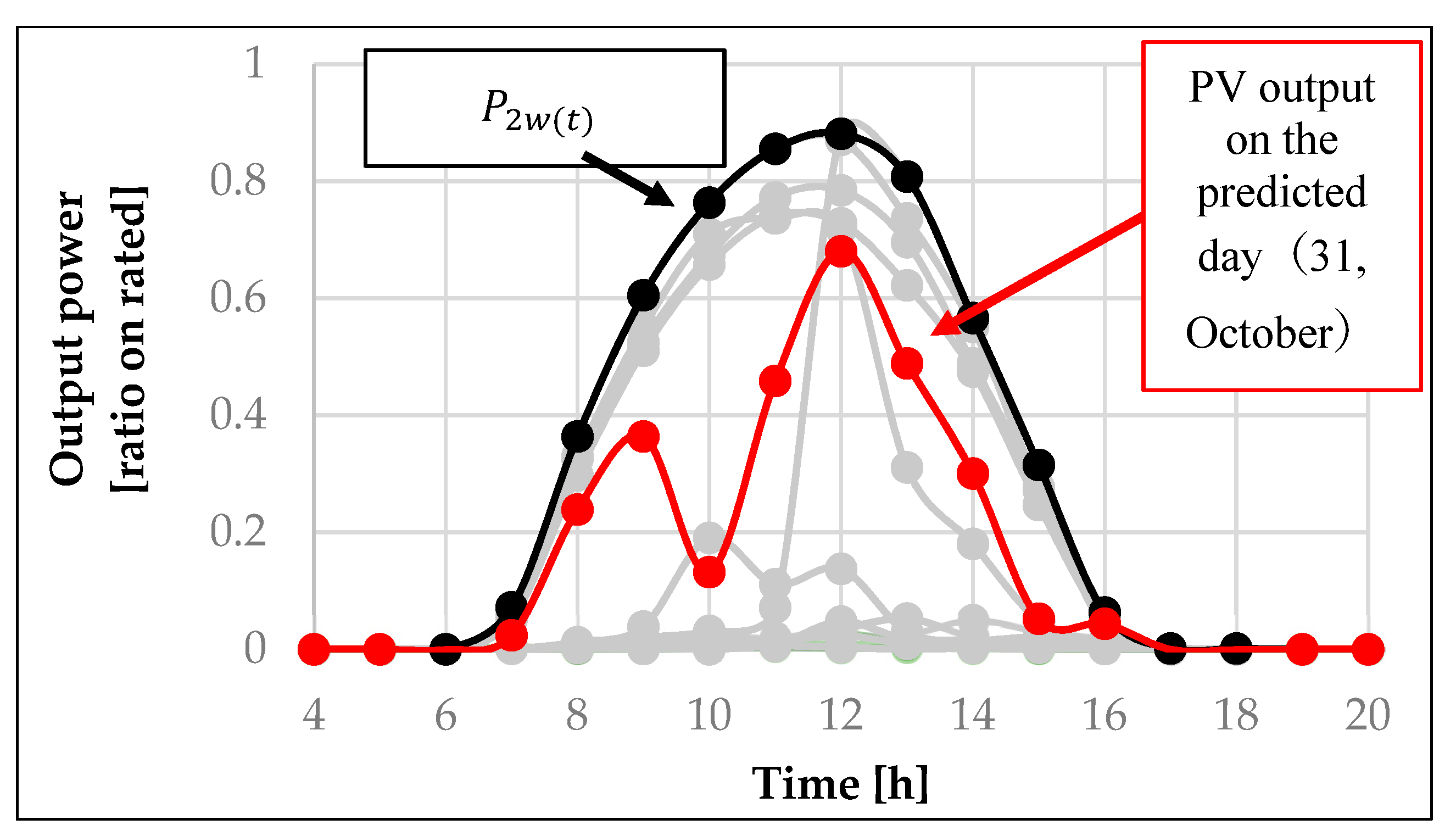
2.1. Normalization

This paper proposes a method to forecast the future output power of PV systems by estimating the motion of the geographical distribution based on the variation of their previous values. However, it is not appropriate to compare the raw values of the output power of respective PV systems, because each PV system differs in terms of the rated power and tilt and azimuthal angles. Various methods have employed normalization to deal with this issue [18]. The method proposed in this paper also normalizes the PV outputs; however, this normalization method is slightly different from the other methods. The NV can be determined using (1).

$$NV=\frac{P\left(t\right)}{P_{2w}\left(t\right)},$$

(1)

where P(t) is the actual output power at a specific time t, and $P_{2w}\left(t\right)$ is the highest output power among the 14 data points at a specific time t in the immediate two weeks (14 days). Lonij et al. [30] employed a similar estimation technique to other normalization methods, using 80% of clear sky performance measurements taken at the same time of day on the previous 15 days in order to normalize the PV output. Figure 1 shows a conceptual graph of $P_{2w}\left(t\right)$. The 14 light-green curves are the output power profiles on the immediate 14 days from 16 October to 30 October, and the red and black curves indicate P(t) and $P_{2w}\left(t\right)$ at each time on the predicted day (31 October), respectively. A two-week term was employed for $P_{2w}\left(t\right)$ to consider seasonality, such as changes in the solar altitude and surrounding environment, and to obtain sunny weather at least once for each time in a period of two weeks.

Kondoh and Kameda [31] previously applied this normalization method to trouble detection by comparing neighboring PV systems. They found that the method can cancel the influence of the rated power and tilt and azimuthal angles on output power by direct solar irradiance, but it cannot cancel the influence on output power by indirect solar irradiance.

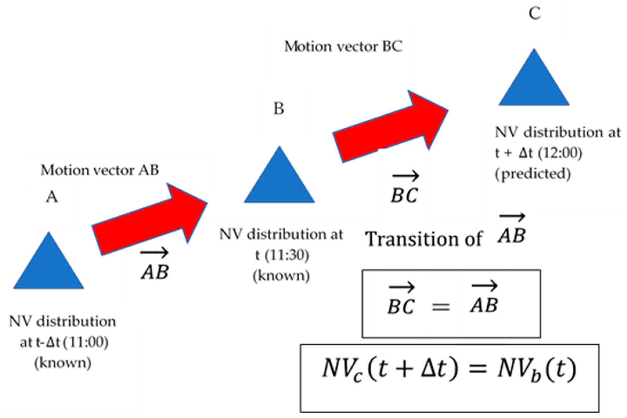
2.2. Motion Estimation

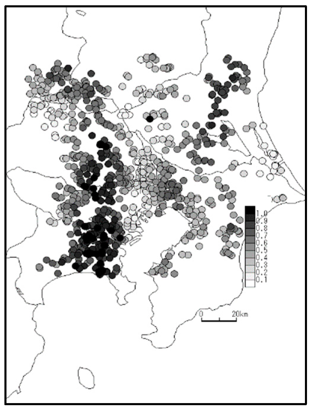
In this method, the geographical distribution of past NVs is assumed to move with time based on the movement of the clouds, and the future PV output is predicted by estimating the motion vectors of the NV distribution. To estimate the motion vectors of the NV distribution, this method uses motion estimation [32], which is a technique developed for image processing. The forecasting process based on motion estimation is as follows.

It is necessary to fix the randomly scattered PV systems to align the pixels in order to apply motion estimation. Figure 2 shows the locations of the monitored PV systems, indicated by respective circles, in the Kanto region of Japan; the tints of the circles indicate the NVs. These distributions are modified to the aligned distributions with meshes, which are distinguished in terms of the latitude and longitude. Figure 3 shows an example of the meshes at 12:00 on 26 September. The tints of the circles in Figure 3 indicate the representative values obtained as averages of the NVs in the respective meshes.

Assuming a uniform linear motion in a very short period, Kameda et al. [32] predicted the linear motion of the NVs. For an NV expressed as $f\left(\mathit{x},t\right)$, the NVs at times t−$\Delta \mathrm{t}$ and t can be expressed as (2):

$$f\left(\mathit{x}-\mathit{u}\left(\mathit{x},t\right)\Delta t,t-\Delta t\right)=f\left(\mathit{x},t\right),$$

(2)

where $\mathit{x}$ is the location of the NV, $\mathit{u}\left(\mathit{x},t\right)$ is the motion vector of the NV at location $\mathit{x}$ and time $t$, and $\mathit{u}\left(\mathit{x},t\right)$ is the velocity at time $\Delta t$. In addition, $\mathit{u}\left(\mathit{x},t\right)={\left(u\left(\mathit{x},t\right),v\left(\mathit{x},t\right)\right)}^T$, where $u\left(\mathit{x},t\right)$ and $v\left(\mathit{x},t\right)$ are the latitude and longitude components, respectively, in which $u\left(\mathit{x},t\right)$ is the velocity of the latitude direction and $v\left(\mathit{x},t\right)$ is the velocity of the longitude direction. The data term $E_D$ and the regularization (spatial smoothing) term $E_s$ of motion distribution are respectively defined in (3) and (4):

$$E_D{}^2\left(\mathit{u},\mathit{x},t\right)={\left(f\left(\mathit{x}-\mathit{u}\left(\mathit{x},t\right)\Delta t,t-\Delta t\right)-f\left(\mathit{x},t\right)\right)}^2$$

(3)

$$E_s\left(\mathit{u},\mathit{x},t\right)=({\left|\nabla u\left(\mathit{x},t\right)\right|}^2+{\left|\nabla v\left(\mathit{x},t\right)\right|}^2),$$

(4)

where $\nabla ={\left({\partial }_x,{\partial }_y\right)}^T$, and $\partial$ is the partial differential operator. The regularization term $E_s$ represents the spatial change of the motion distribution function $\mathit{u}\left(\mathit{x},t\right)$. Using the weighted sum of these terms, we can define the energy function as follows:

$$J\left(\mathit{u},t\right)=\int \left(E_D{}^2\left(\mathit{u},\mathit{x},t\right)+\lambda E_S\left(\mathit{u},\mathit{x},t\right)\right)dx.$$

(5)

Here, $\lambda$ is the weight of the regularization term. In this study, $\lambda$ was set to 1.000 based on the results of preliminary experiments conducted by us. As this is a problem involving the minimization of $J\left(u,t\right)$, the solution is expressed in (6) and (7), which are Euler–Lagrange equations:

$$\mathsf{\lambda }{\nabla }^T\nabla u-E_D{\partial }_{x}f=0,$$

(6)

$$\mathsf{\lambda }{\nabla }^T\nabla v-E_D{\partial }_{y}f=0,$$

(7)

where ${\nabla }^T\nabla =\left({\partial }_x{}^2+{\partial }_y{}^2\right)$, which is a Laplacian function. The details of the solutions to these equations and the corresponding algorithm are given in [32]. Figure 4 presents a conceptual illustration of motion estimation. Using the motion estimation technique, the motion vector AB is first calculated using the NVs at locations A and B. The vector AB is then translated to a vector BC to predict the NV at location C. The NV at location C at t+$\Delta t$ is equal to that at the location of A at t−$\Delta t$ and B at t. For example, the future NV at location C at 12:00 is equal to the NV at location B at 11:30 and location A at 11:00. The future NV is then reconverted to future PV output power using (1).

2.3. Dataset

The dataset used in this study contained actual PV output power with 30 min observation intervals ($\Delta \mathrm{t}$), from August 2013 to July 2014, for approximately 5000 PV systems monitored in Japan. The proposed method used the actual output power data at time t and 30 min prior (t−$\Delta \mathrm{t}$) to estimate the output power at 30 min ahead (t+$\Delta \mathrm{t}$). This study focused on the Kanto region in Japan, which lies in latitude range 35.4–36.5° and longitude range 139.0–140.8°. The number of monitored PV systems was approximately 1200, and their total rated power was approximately 12 MW. When the size of the meshes was reduced to determine the optimal size, some meshes did not contain any PV systems, as shown in Figure 5a, wherein the red circles indicate the missing NVs. The motion estimation technique cannot be used if there are many missing values, such as in Figure 5a. To overcome this problem, the scattered missing values were interpolated using the grid data function in MATLAB R2018a. Various interpolation methods exists; however, griddata was used for simple interpolation in this study. Figure 5b shows the interpolation results. Some values remain missing on the right side; however, the region corresponding to the missing values is largely on the ocean and along the edges. Therefore, the values of these regions do not affect the motion estimation.

2.4. Error Assessment Method

Assesment Method

This method forecasts the output power 30 min ahead. To verify the accuracy, the mean absolute percentage error (MAPE) ((8)) and root mean square error (RMSE) ((9)) were used:

$$MAPE=\frac{1}{N}{{\displaystyle \sum }}_{i=1}^N\frac{\left|P_{rea{l}_i}-P_{forecas{t}_i}\right|}{P_{rat{e}_i}}$$

(8)

$$RMSE=\sqrt{\frac{{{\displaystyle \sum }}_{i=1}^N{\left(P_{rea{l}_i}-P_{forecas{t}_i}\right)}^2}{N}}$$

(9)

where N is the number of PV systems, and $P_{rea{l}_i}$, $P_{forecas{t}_i}$, and $P_{rat{e}_i}$ are the actual PV output, forecasted PV output, and rated power of the i^th PV system, respectively. Equations (10) and (11) were also used to evaluate the optimal mesh size:

$$MAP{E}_{rep}=\frac{1}{M}{{\displaystyle \sum }}_{j=1}^M\left|N{V}_{re{p}_j}-N{V}_{forecas{t}_j}\right|,$$

(10)

$$MAP{E}_{NV}=\frac{1}{N}{{\displaystyle \sum }}_{i=1}^N\left|N{V}_{rea{l}_i}-N{V}_{forecas{t}_i}\right|,$$

(11)

where M is the number of meshes, $N{V}_{ re{p}_j}$ is the actual representative value, which is the average of the output power of all the PV systems in the j^th mesh, $N{V}_{forecas{t}_j}$ is the forecasted NV in the j^th mesh, and $N{V}_{rea{l}_i}$ is the actual NV of the i^th PV system. The two parameters were set to evaluate the rounding error in each mesh. The difference between $MAP{E}_{rep}$ and $MAP{E}_{NV}$ represents the error when some PV systems in a mesh are grouped, and a representative value is used to forecast using the motion estimation. However, the representative values have rounding errors because the representative value is only the average of the NVs, which differ for different PV systems. Optimizing the mesh size helps to decrease the variance in the NVs in one mesh and the rounding error. Equation (10) was used to calculate the error between the actual representative NVs and the forecasted NVs. Equation (11) was used to calculate the error between the actual NVs of the respective PV systems and the forecasted NVs. When the difference between these errors is small, the rounding errors are also small.

3. Results

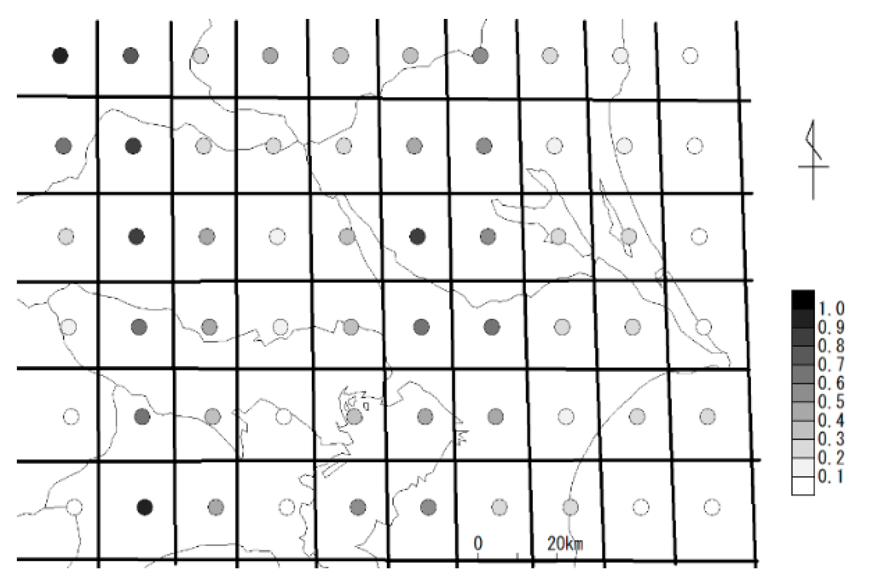
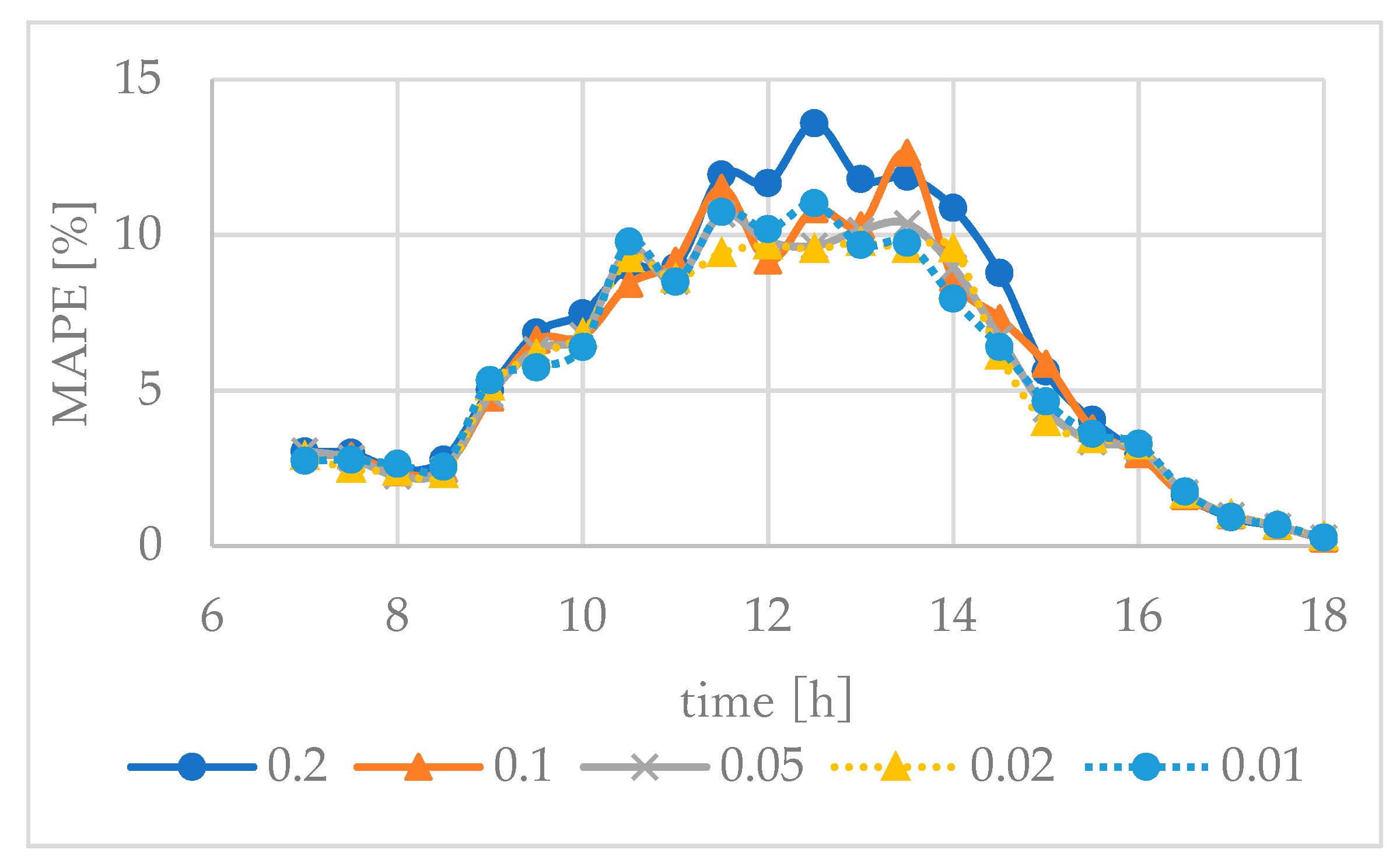
3.1. Optimization of Mesh Size

First, the result for 26 September 2013 is focused on in this section to optimize the size of the mesh. There was a typhoon at sea toward the east of the Kanto region on this day. Therefore, the weather changed drastically, and the PV output change was also drastic. As shown in Figure 2, the NVs for the Kanto region differed significantly from place to place on this day. As the NVs significantly differ even within a mesh, the optimum mesh size for this day is considered to be the optimum mesh sizes for other days as well. Figure 6a–e shows the $MAP{E}_{rep}$ and $MAP{E}_{NV}$ profiles with every 30 min forecast for several mesh sizes. Comparing Figure 6a–d, we find that, the lower the mesh width is, the closer are the two curves. These results show that the rounding errors can be decreased by reducing the width of the mesh up to 0.02° (1.8 km) in both latitude and longitude. Comparing Figure 6d,e, it can be seen that there is little difference between them. To optimize the mesh size, the MAPE of the non-NVs ($MAP{E}_{rep}$ in Equation (10)) and the output powers of the respective PV systems (MAPE in Equation (8)) are considered next. Figure 7 shows the MAPE between the actual and forecasted output powers of the respective PV systems. The smaller the mesh is, the lower is the MAPE up to 0.02° (1.8 km). However, the MAPE curve of 0.02° (1.8 km) is lower than that of 0.01° (0.9 km), particularly around noon, as shown in Figure 7. Furthermore, the daily average of the MAPE of 0.02° (1.8 km) is 5.39% and that of 0.01° (0.9 km) is 5.53%. Therefore, a mesh size of 0.02° (1.8 km) is the most suitable for this method.

3.2. Result and Comparison with Other Methods

Figure 8a shows the result of the output power forecast for a sunny day on 19 September 2013 in terms of the total output power of all the PV systems forecasted. The MAPEs calculated using (8) are lower than 2.5% on this day, averaging at 1.97%. These values indicate that the MAPEs are low when the day is sunny; this is expected because the output power of PV systems is known to follow a sinusoidal curve on a sunny day, in general.

Figure 8b shows the result of the output power forecast for 8 October 2013. On this day, the weather was sunny in the morning and cloudy in the afternoon. The daily average of the MAPE was 5.86% on this day.

Figure 8c shows the result for 23 September 2013; the weather was cloudy in the morning and rainy in the afternoon. The total output power after 11:00 was much lower than that on 8th October 2013. The daily average of the MAPE on the day was 5.40%. These results show that the proposed method can accurately forecast the total output power on cloudy days as well.

Figure 8d shows the result for a rainy day on 6 June 2014, with less generation output. The daily average of the MAPE on the day was 2.51%. Even on a rainy day, the accuracy of the forecast is high; however, this is natural because the total output power on a rainy day is low compared with the total rated power in the entire Kanto region, and the prediction of such a low output power exhibits a low error in Equation (8).

Table 1. Error in forecasting total output power.

Date	Weather Condition	MAPE [%]	RMSE [kW]
19 September 2013	Sunny	1.97	0.36
23 September 2013	Cloudy and rainy	5.40	0.85
8 October 2013	Cloudy and sunny	5.86	0.93
6 June 2014	Rainy	2.51	0.46
26 September 2013	Significant change	5.39	0.87
	average	4.23	0.69

lists the RMSE and average of daily MAPE for five days in Figure 8. The value in the bottom row represents the average of MAPE and RMSE for five days. These low values show the effectiveness of this study.

To verify the accuracy of the proposed method, the RMSEs obtained using the forecast methods proposed by Zang et al. [33], Seyedmahmoudian et al. [34], and Zhou et al. [35] were compared to that obtained using the proposed method.

Table 2. RMSE comparison with other methods.

Method	Total Rated Power	Number of PV Systems	Forecast Horizon	RMSE
Neural network (Zang et al. [33])	100 kW	No description	1 h	2.05
Metaheuristic approach (Seyedmahmoudian et al. [34])	3 kW	1 system	1 h	4.40
Neural network and attention mechanism (Zhou et al. [35])	20 kW	2 systems	30 min	1.81
Proposed method	12 MW	1200 systems	30 min	0.69

lists the RMSE values of the four methods. The RMSE average of the proposed method is 0.69 kW, which is much lower than those of the other four methods. However, the proposed method forecasts the output power 30 min ahead, whereas the methods by Zang et al. [33] and Seyedmahmoudian et al. [34] forecast one hour ahead. The shorter the forecast time horizon is, the better is the performance. However, despite the difference in the time horizons being only 30 min, the difference in the RMSEs is significant. This shows that the proposed method with the geographical distribution can be used to effectively forecast the output power.

3.3. Reasons for Error

Two reasons can be deduced for the errors observed in the proposed method. The first is the normalization of the output power. The normalization was done to compare the output powers of the PV systems, which have different tilt and azimuthal angles and rated power. However, the differences exhibited by the respective PV systems cannot be completely cancelled out by normalization. This is the reason for the error when normalization is performed.

The other reason is the motion estimation. Figure 8e shows the result for 26 September 2013, wherein the MAPE recorded the highest value of 9.77% at 13:00. Let us focus on this time to understand the reason for the error. Figure 9a–c show the distribution of the NVs from 12:00 to 13:00. Figure 10 shows the image of the motion vectors estimated for the forecast at 13:00. Figure 9 shows a wide area with high NVs moving from west to east in the western part of the Kanto region and from northwest to southeast in the northern part (indicated using a red square frame in Figure 10) of the Kanto region. By comparing the movements shown in Figure 10, we find that the directions of the movement of the actual NVs are largely consistent with the directions of the motion vectors. However, the directions of the motion vectors in the northern part of the Kanto region are estimated to be toward northeast and not southeast. This results in another error because of the difference between the directions of the actual and estimated movements of the NVs.

4. Conclusions

This paper proposed a direct method for forecasting the output power of geographically distributed PV systems using their previous dataset. Learning methods, such as SVM and NN, have often been used for forecasting PV output. The proposed method is different from these approaches, as it estimates the movement of the geographical distributions of the NVs of the output power. To forecast the output power, the previous output power is first normalized. Then, the geographical distributions of the NVs of the respective PV systems are modified to aligned meshes, and a motion estimation technique is applied to forecast the future movements of the NVs. Finally, the future NVs are reconverted to the future output power of the respective PV systems. The averages of the MAPE and RMSE for the proposed method were, respectively, 4.23% and 0.69 kW. The errors occur in the processes of normalization and averaging in meshes and motion estimation, but the low MAPE and RMSE verify the high accuracy of this method. Thus, we believe the proposed method can be used to effectively forecast the output power of geographically distributed PV systems.

The following further studies should be conducted in the future:

• Correlation between the available amount of data of PV systems and prediction accuracy: All the data we could obtain were used to forecast with the best prediction accuracy in this study. However, we hypothesize that the prediction accuracy depends on the available data. Therefore, it is important to investigate their relationship and to determine the minimum amount of data with which forecasting can be done with a tolerable accuracy.
• The proposed method only forecasts the output power at 30 min ahead, which is the same period as the sampling interval of the data used for the forecast processes. Forecasting other time horizons and evaluating the corresponding error should be performed.
• In the motion estimation, only the two historical points of PV outputs were used while assuming uniform linear motion, as shown in Figure 4. However, there is a possibility that using more history points could improve prediction accuracy, for example, by capturing spiral motion.

References

1. Renewables 2018 Global Status Report; Ren 21: Paris, France, 2018; ISBN 978-3-9818911-3-3. Available online: https://www.ren21.net/wp-content/uploads/2019/08/Full-Report-2018.pdf (accessed on 21 October 2019).
2. Flexible Resources to Help Renewables–Fast Facts 2016. California Independent System Operator. 916.351.4400. California, America. 10 November 2016. Available online: https://www.caiso.com/Documents/FlexibleResourcesHelpRenewables_FastFacts.pdf (accessed on 21 October 2019).
3. Ohtake, H.; Shimose, K.I.; Fonseca, J.G.S., Jr.; Takashima, T.; Oozeki, T.; Yamada, Y. Accuracy of the solar irradiance forecasts of the Japan Meteorological Agency mesoscale model for the Kanto region, Japan. Sol. Energy 2013, 98, 138–152. [Google Scholar] [CrossRef]
4. Mellit, A.; Pavan, A.M. A 24-h forecast of solar irradiance using artificial neural network: Applications for performance prediction of a grid-connected PV plant at Trieste, Italy. Sol. Energy 2010, 84, 807–821. [Google Scholar] [CrossRef]
5. Wang, F.; Mi, Z.; Su, S.; Zhao, H. Short-Term Solar Irradiance Forecasting Model Based on Artificial Neural Network Using Statistical Feature Parameters. Energies 2012, 5, 1355–1370. [Google Scholar] [CrossRef] [Green Version]
6. Marquez, R.; Coimbra, C.F.M. Forecasting of global and direct solar irradiance using stochastic learning methods, ground experiments and the NWS database. Sol. Energy. 2011, 85, 746–756. [Google Scholar] [CrossRef]
7. Thorey, J.; Mallet, V.; Chaussin, C.; Descamps, L.; Blanc, P. Ensemble forecast of solar radiation using TIGGE weather forecasts and HelioClim database. Sol. Energy 2012, 120, 232–243. [Google Scholar] [CrossRef]
8. Available online: https://www.ecmwf.int/en/research/projects/tigge (accessed on 21 October 2019).
9. Available online: http://www.soda-pro.com/ (accessed on 21 October 2019).
10. Yamazaki, T.; Homma, H.; Wakao, S.; Fujimoto, Y.; Hayashi, Y. Estimation Prediction Interval of Solar Irradiance Based on Weather Classificastion and Support Vector Machines. Electr. Eng. Jpn. 2015, 135, 160–167. [Google Scholar]
11. Jamaly, M.; Kleissl, J. Spatiotemporal interpolation and forecast of irradiance data using Kriging. Sol. Energy 2017, 158, 407–423. [Google Scholar] [CrossRef]
12. Yang, D.; Dong, T.; Reindl, T.; Jirutitijaroen, P.; Walsh, M.W. Solar irradiance forecasting using spatio-temporal empirical kriging and vector autoregressive models with parameter shrinkage. Sol. Energy. 2014, 103, 550–562. [Google Scholar] [CrossRef]
13. Liaoliao, W.; Chenggang, C.; Ning, Y.; Hui, C. Evaluation of solar irradiance on inclined surfaces models in the short-term photovoltaic power forecasting. J. Eng. 2017, 2017, 2226–2230. [Google Scholar] [CrossRef]
14. Pelland, S.; Remund, J.; Kleissl, J.; Oozaki, T.; Brabandere, D.K. Photovoltaic and Solar Forecasting: State of the Art. In International Energy Agency Photovoltaic Power Systems Programme; Technical Report IEA-PVPS T14-01; International Energy Agency: Paris, France, 2013. [Google Scholar]
15. Rubby, N.; Jayabarathi, R. Prediction the Power Output of a Grid-Connected Solar Panel Using Multi-Input Support Vector Regression. Procedia Comput. Sci. 2017, 115, 723–730. [Google Scholar]
16. Fonseca, J.G.; Oozaki, T.; Takashima, T.; Koshimizu, G.; Uchida, Y.; Ogimoto, K. Use of support vector regression and numerically predicted cloudiness to forecast power output of a photovoltaic power plant in Kitakyushu, Japan. Prog. Photovolt. Res. Appl. 2012, 20, 874–882. [Google Scholar] [CrossRef]
17. Pierro, M.; Felice, D.M.; Maggioni, E.; Moser, D.; Perotto, A.; Spada, F.; Gornaro, G. Data-driven upscaling methods for regional photovoltaic power estimation and forecast using satellite and numerical weather prediction data. Sol. Energy 2017, 158, 1026–1038. [Google Scholar] [CrossRef]
18. Liu, Y.; Li, K.; Bai, K.; Zhang, Z.; Lu, X.; Zhang, K. Short-term power-forecasting method of distributed PV power system for consideration of its effects on load forecasting. J. Eng. 2017, 13, 865–869. [Google Scholar] [CrossRef]
19. Liu, W.; Liu, C.; Lin, Y.; Ma, L.; Xiong, F.; Liu, J. Ultra-Short-Term Forecast of Photovoltaic Output Power under Fog and Haze Weather. Energies 2018, 11, 528–550. [Google Scholar]
20. Yang, H.T.; Huang, C.M.; Huang, Y.C.; Pai, Y.S. A Weather-Based Hybrid method for 1-Day Ahead Hourly Forecasting of PV Power Output. IEEE Trans. Sustain. Energy 2014, 5, 917–926. [Google Scholar] [CrossRef]
21. Killinger, S.; Braam, F.; Muller, B.; Wille-Haussmann, B.; Mckenna, R. Projection of power generation between differently-oriented PV systems. Sol. Energy 2016, 136, 153–165. [Google Scholar] [CrossRef]
22. Inman, R.H.; Pedro, H.T.C.; Coimbra, C.F.M. Solar forecasting methods for renewable energy integration. Prog. Energy Combust. Sci. 2013, 39, 535–576. [Google Scholar] [CrossRef]
23. Antonanzas, J.; Osorio, N.; Escobar, R.; Urraca, R.; Martinez-de-Pison, F.J.; Antonanzas-Torres, F. Review of photovoltaic power forecasting. Sol. Energy 2016, 136, 78–111. [Google Scholar] [CrossRef]
24. Yang, D.; Kleissl, L.; Gueymard, C.A.; Pedro, H.T.C.; Coimbra, C.F.M. History and trends in solar irradiance and PV power forecasting: A preliminary assessment and review using text mining. Sol. Energy 2018, 168, 60–101. [Google Scholar] [CrossRef]
25. Kito, S.; Kurimoto, M.; Kato, T.; Suzuki, Y.; Manabe, Y.; Funabashi, T. A study on Satellite Image-Based Forecasting of Ramp Events of Spatial Average Irradiance. In Proceedings of the Joint Technical Meeting on Frontier Technology and Engineering and Metabolism Society and Environmental Systems, FTE-15-005/MES-15-005. Nagoya, Japan, 15–16 January 2015. (In Japanese). [Google Scholar]
26. Lorenz, E.; Hammer, A.; Heinmann, D. Short term forecasting of solar radiation based on satellite data. In Proceedings of the EUROSUN2004 (ISES Europe Solar Congress), Freiburg, Germany, 20–23 June 2004. [Google Scholar]
27. Chow, C.W.; Belongie, S.; Kleissl, J. Cloud motion and stability estimation for intra-hour solar forecasting. Sol. Energy 2015, 115, 645–655. [Google Scholar] [CrossRef]
28. Bernecker, D.; Riess, C.; Angelopoulou, E.; Hornegger, J. Continuous short-term irradiance forecasts using sky images. Sol. Energy 2014, 110, 303–315. [Google Scholar] [CrossRef]
29. Miyazaki, Y.; Kondoh, J.; Kameda, Y. Forecasting System Using Actual Multipoint PV Output. In Proceedings of the Grand Renewable Energy, O-Pv-8-5, Yokohama, Japan, 17–22 June 2018. [Google Scholar]
30. Lonij, V.P.; Brooks, A.E.; Koch, K.; Cronin, A.D. Analysis of 80 rooftop PV systems in the Tuscon, AZ area. In Proceedings of the 2012 38th IEEE Photovoltaic Specialists Conference, Austin, TX, USA, 3–8 June 2012. [Google Scholar]
31. Kondoh, J.; Kameda, Y. Trouble Detection by Comparing Power Generation by Neighbor PV Systems. Tech. J. Smart Grid 2017, 58, 27–32. (In Japanese) [Google Scholar]
32. Kameda, Y.; Kishi, H.; Ishikawa, T.; Matsuda, I.; Itoh, S. Multi-frame motion compensation using extrapolated frame by optical flow for lossless Video Coding. In Proceedings of the 2016 IEEE International Symposium on Signal Processing and Information Technology, Limassol, Cyprus, 12–14 December 2016. [Google Scholar]
33. Zhang, H.; Cheng, L.; Ding, T.; Cheung, K.W.; Liang, Z.; Wei, Z.; Sun, G. Hybrid method for short-term photovoltaic power forecasting based on deep convolutional neural network. IET Gener. Transm. Distrib. 2018, 12, 4557–4567. [Google Scholar] [CrossRef]
34. Seyedmahmoudian, M.; Jamei, E.; Thirunavukkarasu, G.S.; Soon, T.K.; Mortimer, S.; Horan, B.; Stojcevski, A.; Mekhilef, S. Short-Term Forecasting of the Output Power of a Building-Integrated Photovoltaic System Using a Metaheuristic Approach. Energies 2018, 11, 1260–1282. [Google Scholar] [CrossRef] [Green Version]
35. Zhou, H.; Zhang, Y.; Yang, L.; Liu, Q.; Yan, K.; Du, Y. Short-Term Photovoltaic Power Forecasting Based on Long Short Term Memory neural Network and Attention Mechanism. IEEE Access 2019, 7, 78063–78074. [Google Scholar] [CrossRef]
Figure 1. Conceptual diagram of normalized values.
Energies 12 04815 g001
Figure 2. NV distribution around Kanto region in Japan (12:00, 26 September 2013).
Energies 12 04815 g002
Figure 3. Distribution of representative NVs (12:00, 26 September 2013).
Energies 12 04815 g003
Figure 4. Conceptual illustration of motion estimation.
Energies 12 04815 g004
Figure 5. Distribution of representative NVs in respective meshes on 26 September 2013 (The grid size is 0.05 degrees (4.5 km) in latitude and 0.05 degrees in longitude.), (a) Before interpolation, (b) After interpolation using MATLAB.
Energies 12 04815 g005
Figure 6. MAPE in forecasting normalized values (26 September 2013). (a) Case of 0.2° (18 km) in both latitude and longitude. (b) Case of 0.1° (9 km) in both latitude and longitude. (c) Case of 0.05° (4.5 km) in both latitude and longitude. (d) Case of 0.02° (1.8 km) in both latitude and longitude. (e) Case of 0.01° (0.9 km) in both latitude and longitude.
Energies 12 04815 g006
Figure 7. MAPE of PV output (26 September 2013).
Energies 12 04815 g007
Figure 8. Result of forecasting total output power. (a) Sunny day (19 September 2013), (b) Sunny and cloudy day (8October 2013), (c) Cloudy and rainy day (23 September 2013), (d) Rainy day (6 June 2014), (e) Drastically changing weather (26 September 2013).
Energies 12 04815 g008
Figure 9. Distribution of NVs (26 September 2013). (a) 12:00; (b) 12:30; (c) 13:00.
Energies 12 04815 g009
Figure 10. Motion estimation vectors (12:00, 26 September 2013).
Energies 12 04815 g010