Abstract
In the transmission expansion planning (TEP) problem, it is challenging to consider a fault current level constraint due to the time-consuming update process of the bus impedance matrix, which is required to calculate the fault currents during the search for the optimal solution. In the existing studies, either a nonlinear update equation or its linearized version is used to calculate the updated bus impedance matrix. In the former case, there is a problem in that the mathematical formulation is derived in the form of mixed-integer nonlinear programming. In the latter case, there is a problem in that an error due to the linearization may exist and the change of fault currents in other buses that are not connected to the new transmission lines cannot be detected. In this paper, we use a method to obtain the exact updated bus impedance matrix directly from the inversion of the bus admittance matrix. We propose a novel method based on the inverse matrix modification lemma (IMML) and a valid inequality is proposed to find a better solution to the TEP problem with fault current level constraint. The proposed method is applied to the IEEE two-area reliability test system with 96 buses to verify the performance and effectiveness of the proposed method and we compare the results with the existing methods. Simulation results show that the existing TEP method based on impedance matrix modification method violates the fault current level constraint in some buses, while the proposed method satisfies the constraint in all buses in a reasonable computation time.
1. Introduction
Because electricity is difficult to store economically, and it can only be delivered through transmission lines, transmission networks must be expanded in proportion to the increase in electricity demand. Even though the expansion of a transmission network provides positive effects, such as reduction of congestion, an increase in system reliability, and a reduction of transmission loss, a side effect of fault current increase (especially near large metropolitan areas) occurs due to the decrease in the impedance of the overall system [1].
Most of the widely used methods solve this problem by splitting buses, installing additional equipment such as a superconducting current limiter, or upgrading the circuit breaker with a higher breaking capacity. However, one of the more fundamental solutions to solve this problem is to consider the fault current level during transmission expansion planning (TEP), which is the main topic of this paper.
In general, the capacity of a circuit breaker is chosen to be greater than the three-phase line-to-ground fault current, which is calculated as the pre-fault voltage divided by the Thévenin equivalent impedance. In power system optimization problems with short time horizons, such as the optimal power flow or security constraint unit commitment, it can be assumed that the network configuration is fixed, and the fault current can be considered as linear constraint or upper bound on the bus voltage magnitude [2,3,4]. However, in a problem with a relatively long time horizon, it becomes mathematically challenging to consider the fault current in the optimization problem, because the bus impedance matrix is continuously changing.
Research on the TEP problem that considers fault current has been published only recently, and there are two reasons why the fault current has not been studied in the TEP problem in the past. The first is that the commercially available circuit breaker has a sufficient breaking capability margin, compared to the fault current possible in the system, and the second is that the computational burden has been too large to account for the fault current in the TEP problem. There is limited research on the fault current in the TEP problem [5,6,7,8]. The most important feature of these studies is summarizing how to reduce the calculation burden due to updating the system matrix (the bus impedance matrix), which is essential for calculation of the fault current.
For example, in order to overcome this problem, previous research used a metaheuristic algorithm such as the genetic algorithm (GA), removed infeasible cases by applying the Benders cut, or simplified the problem by linear approximation. However, the GA algorithm has a problem in that it cannot reproduce the same results due to the inherent randomness of the algorithm, not to mention its slow convergence [5]. Additionally, methods based on Benders decomposition must solve the problem repeatedly until infeasible cases do not occur, and hence, the number of iterations required to find the optimal solution increases exponentially as the number of candidates for the new transmission line increases [6]. In the linear approximation method, even though the method can find the solution in a relatively short period of time, there is a disadvantage in that the calculation result of the fault current may differ significantly from the actual value due to the model error brought about by the linearization process [7,8]. As a result, most of the existing methods have a problem in that the calculation time is too slow or the accuracy is too limited to be applied to an actual large-scale power system. It should be noted that our study is confined to the balanced fault such as three-phase line-to-ground fault. For power systems where the unbalanced faults are dominant, such as distribution systems, special methods are employed to calculate power flow and fault current, as described in [9,10].
Therefore, the main purpose of this paper is to propose a more exact and efficient method to solve the TEP problem with a fault current level constraint based on the inverse matrix modification lemma (IMML) and a valid inequality. The proposed method consists of the following two steps.
The first is to efficiently calculate the diagonal terms of the bus impedance matrix, which is the Thévenin equivalent impedance of the system [11], and this bus impedance matrix should be recalculated repeatedly during the optimization process. In the existing research [7], a linearized and simplified version of the nonlinear impedance update equation is used to formulate the resulting optimization problem into mixed integer linear programming (MILP) form. The authors of [7] concluded that the normalized root mean square (RMS) error of about 2–3% due to linearization is a minor problem from a practical standpoint. However, in some power systems, such as those in South Korea, where the margins between the fault current and the circuit breaking capability are very narrow, more exact calculation of the fault current is required. Another problem with the method used in [7] is that it cannot guarantee the accuracy of the fault current calculation results at other buses to which the new transmission lines are not connected directly.
In this paper, in order to avoid these problems, the updated bus impedance matrix is calculated from the inversion of the bus admittance matrix. As will be explained in the following sections, this method does not require the nonlinear update equation for calculating the bus impedance matrix, and therefore, the overall optimization problem can be formulated as a MILP optimization problem without linearization. Additionally, the fault currents at the other buses to which the added transmission line is not directly connected can also be calculated without error.
The disadvantage of this method is obviously that the inverse of the bus admittance matrix must be calculated repeatedly in the search for the optimal solution to the TEP problem. In order to mitigate the computational burden of computing the inverse of the bus admittance matrix at every step to find the optimal solution to the TEP problem, we apply the inverse matrix modification lemma (IMML) and the valid inequality.
Due to the nature of the TEP problem, only a part of the transmission network is slightly changed during the search for the optimal solution. Therefore, it has a structure that is well suited to applying the well-known IMML, which can help to calculate the inverse of the bus admittance matrix efficiently [12]. A linear update equation for the diagonal terms of the bus impedance matrix will be explained in detail in the later sections.
Even though the time to calculate the updated impedance can be reduced greatly by using the IMML, the overall computation time to find the optimal solution to the TEP problem still becomes intractable as the number of candidates for new transmission lines increase. Thus, in this paper, we have devised a new method based on a valid inequality to reduce the feasible area of the problem. The valid inequalities are generated every search step during the optimization and added as additional inequality constraints to branch-and-cut (B&C) algorithm to reduce the feasible search region. As shown in the simulation section, the combination of the IMML and the proposed valid inequality can find the optimal solution to the TEP problem with consideration of the fault current very accurately in a reasonable calculation time.
The rest of this paper is organized as follows: Section 2 explains the MILP formulation of the TEP problem with the fault current level constraint. The method used for the solution in this study, based on the B&C algorithm, and the suggested valid inequality method are explained in Section 3. The proposed method is applied to IEEE Reliability Test System with 96 buses (RTS-96), which is frequently used in studies for the TEP problem. The simulation results and the concluding remarks are summarized in Section 4 and Section 5, respectively. Nomenclature describes of all parameters and variables used in this paper.
2. Mathematical Formulation
2.1. Objective Function
The objective function used in this paper has a form similar to that used in the general TEP problem, which is composed of generator operation cost, transmission line construction cost, and salvage value of the transmission lines, as follows:
where is the linearized generation cost function given as follows:
which can be further simplified into the following equation:
2.2. Fault Current Constraints
2.2.1. Conventional Method for the Bus Impedance Update
Generally, the three-phase line-to-ground fault current can be calculated by the following equation:
where and are the pre-fault voltage and Thévenin equivalent impedance at bus , respectively. Since Thévenin equivalent impedance is the same as the corresponding diagonal element of the bus impedance matrix if the pre-failure voltage is assumed to be 1.0 (pu), the three-phase line-to-ground fault current constraint in the TEP problem can be expressed as follows [13]:
where is the (i,j)th element of bus impedance matrix in year t.
In the existing study, the following update equation is used to calculate each element of the bus impedance matrix after the transmission lines are added [7,8]:
where and are the coefficients for linearization, which can be calculated using the following equations:
In order to improve the computational speed in the process of applying the above equations, the existing studies [7,8] assume that the off-diagonal elements of the bus impedance matrix are negligibly smaller than the diagonal elements (), and the diagonal elements of the bus impedance matrix before the update are significantly smaller than the impedance of the new transmission lines that will be connected to the buses (). Hence, the values of and in Equation (8) are all assumed to be 1. This method has an advantage in that the computational burden for calculating the fault currents can be largely reduced, however, there is a problem in that it is impossible to consider the changes in the fault currents occurring on buses to which the new transmission lines are directly connected. Additionally, as the number of new transmission lines increases, the calculation error is cumulative.
2.2.2. Derivation of the Bus Impedance Update Equation Based on the IMML
In this paper, we adopt a method to directly calculate the bus impedance matrix by inversion of the bus admittance matrix of the new system with the added transmission line, as follows:
It is obvious that the calculation time will significantly increase due to the curse of dimensionality if the system becomes larger. Therefore, it is essential to calculate the inverse matrix more effectively to incorporate the fault current constraint (or Equation (5)). In order to find the optimal solution to the TEP problem, a new transmission network configuration for the next search step is constructed by adding one new transmission line to the network configured in the previous search step. The bus admittance matrix of the next search step will have almost the same value, and only small number of elements in the admittance matrix is changed from the bus admittance matrix of the previous step. Therefore, the following inverse matrix modification lemma can be applied in a very straightforward manner to acquire the updated bus impedance matrix.
The so-called Woodbury equation of the IMML can be described as the following generic equation [12]:
If , the variation of the admittance matrix , can be decomposed into the product of three matrices, or , the new admittance matrix, , can be expressed as follows:
where is the variation of matrix Y (m m), is the connection matrix (n m), is the number of total buses and is the number of modified buses. Here, time index is omitted for simplicity.
By applying the Woodbury equation of the IMML to Equation (12), a new impedance matrix, , can be obtained as follows:
where is the impedance matrix of the previous optimization step. In order to eliminate the unnecessary inverse operation, Equation (14) is replaced with the following equation:
Here, we apply an extra assumption that only one new transmission line can be added to the existing bus in order to derive a more compact formulation for Equation (16). In case that more than one transmission line should be added to a bus, the above assumption is still valid since we can insert a dummy bus between the new transmission line and the existing bus with small reactance between the buses. Therefore, most of the elements in matrix are not changed except for the corresponding elements of the pair of the buses to which the new transmission line candidate is connected. Thus, can be expressed as the following equation:
where and are [(m − 2) × (m − 2)] and [2 × 2] matrices, respectively. Furthermore, the following equations can be obtained by substituting Equation (18) into Equation (16) with appropriate partitioning:
or
Without loss of generality, by appropriate indexing and simple matrix manipulation, we can define subscript A as the set of buses where the transmission line is constructed, and subscript B as the set of buses where the transmission line is not constructed, which means that all elements of in Equation (19) will be zero. Then the following equations can be easily derived from Equation (20) through Equation (23):
It should be noted that both Equation (24) and Equation (25) should be regarded as nonlinear, because they contain terms in the production of two variables: and . In this paper, we apply the following algorithm, which has the same effect as the above equations, so that the resulting optimization problem becomes a MILP formulation.
If , then:
And if xlj = 0, then:
In the above equations, and denote the real and imaginary parts of the product of matrix and matrix , respectively. All logic expressions in the above are implemented using the indicator constraint option of the CPLEX solver incorporated in the General Algebraic Modeling System (GAMS) [14]. Once all the elements of are calculated using Equations (27)−(29), they can be entered into Equation (12), and the equation to calculate the diagonal element of the new bus impedance matrix (or the Thévenin equivalent impedance) is derived as follows:
Generally, the reactance is more dominant than the resistance of the transmission line, thus, it can be assumed that without significant loss of generality. Hence, the constraint given by Equation (5) can be rewritten as follows:
2.3. Other Constraints
The following constraints are incorporated into the model to account for the technical limitations of the power system and its components.
2.3.1. Power Flow Equation
The following typical DC power flow equations are included in the model [13]:
Equation (32) is the DC power flow equation for the existing transmission lines, and Equation (33) is for the candidates to be newly constructed. For the latter, in the search process, constructing () and not constructing () are expressed separately.
2.3.2. Node Balance Equation
The demand and supply condition at each bus is represented as the following equality constraint:
2.3.3. Limit on Generator Output
All the generators should satisfy the following inequality constraints for the limits on the active power output:
In general, in the TEP problem, the on/off status of generator is not considered due to the computational burden. In this paper, for slight improvement of the accuracy of the generation cost, the on/off status of generator is included in the model. However, if the overall computation time is crucial during the simulation, Equation (35) can be simplified to without significant problem.
2.3.4. Transmission Limit
The following inequality constraints should be satisfied to limit the apparent power flow through the transmission lines:
2.3.5. Bus Voltage Angel Limit
The following inequality constraint is included to limit the bus voltage angles:
2.3.6. New Transmission Line Constraint
In this study, we assume that both existing and newly constructed transmission lines will be maintained until the end of the planning period once they are constructed. The following constraints are included in the model for this purpose:
3. Solution Methods
The TEP problem with the fault current constraint formulated in the previous section is a typical MILP optimization problem. One of the most commonly used methods to find the optimal solution of the MILP problem is the branch-and-cut algorithm. In general, the B&C algorithm is known to be able to obtain the optimal solution for a relatively small-scale MILP problem, but as explained in the simulation section, the curse of dimensionality still occurs in the TEP problem when considering the proposed fault current constraint. As a result, when the scale of the system increases, the optimal solution cannot be searched for within a reasonable period of time.
In this section, we propose a valid inequality method that can help efficiently find the optimal solution to a given TEP problem. The valid inequality method is one of the ways to improve the search speed by removing the search space from the feasible region where there is no possibility of the solution in a given optimization problem. For example, valid inequalities are effectively used to improve the performance of the B&C algorithm to solve MILP problems such as the traveling salesman problem [15], unit commitment [16], and the oil pipeline design problem [17]. Since most of the valid inequalities are very problem-specific in nature, the valid inequalities used in the previous studies cannot be applied to the TEP problem. Hence, this study proposes a new valid inequality that is well suited to the proposed TEP problem, and it shows through simulation results that the proposed valid inequality works efficiently. Next, we briefly describe the B&C algorithm and then explain the valid inequality suggested in this study.
3.1. Branch and Cut(B&C) Algorithm
The B&C algorithm is a combination of the branch-and-bound (B&B) algorithm and the cutting plane method. Figure 1 shows a flow diagram of the B&C algorithm used in this study [18].
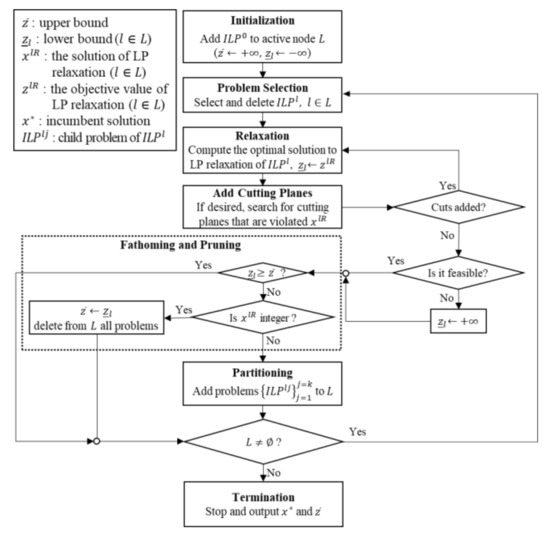
Figure 1.
Flow chart of the branch-and-cut algorithm [18].
3.2. Valid Inequalities
As mentioned above, it is assumed in this paper that the existing transmission lines are not decommissioned during the planning period. We believe that this assumption is reasonable because the existing transmission lines are rarely decommissioned even in an actual situation, and in most cases, the aged lines are maintained through reinforcement works.
The proposed model includes two binary variables, one related to transmission line construction (), and the other to generator operation status (). If a combinatorial set of does not satisfy the fault current constraint, a feasible solution does not exist, whatever values are assigned to . Additionally, in general, as more transmission lines are built, the fault current at each bus tends to increase.
Having said that, we can assert that at least one of the new transmission lines included in the expansion plan should be removed from the plan if a given combination of does not satisfy the fault current constraint. Therefore, the following valid inequality constraint can be added to the mathematical model if the fault current constraint or Equation (5) is not satisfied:
where is the round-off operator. The valid inequality is added as a new constraint to the cutting plane. In this study, the above valid inequality is implemented using the branch-and-cut-and-heuristic (BCH) of GAMS [14].
4. Simulation Results
In order to verify the performance of the proposed method, several simulations were performed on the IEEE RTS-96 system, which is frequently used for the TEP problem [19]. The studied power system is depicted in Figure 2. Additionally, Figure 3 shows the load duration curve used in the study, where the durations of load blocks are 1752 hours for a 100% load, 5256 hours at 80%, and 1752 hours at 40%. The growth rate of annual electricity demand and the discount rate are arbitrarily set at 10% and 7%, respectively. The base power and the upper limit of the fault current in each bus are set to 100 MVA and 10 kA, respectively. Other technical parameters used in the simulations are listed separately in the Appendix A.
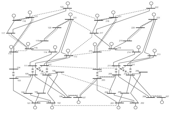
Figure 2.
IEEE two-area RTS-96 system (solid: existing; dashed: candidates).
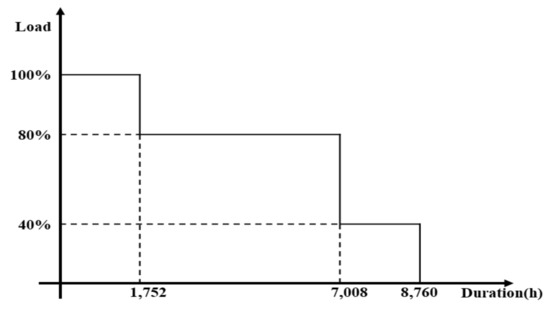
Figure 3.
Load duration curve.
The proposed model was implemented using the CPLEX solver, which is one of the most frequently used MILP solvers available with the General Algebraic Modeling System (GAMS) [20]. In short, the mathematical formulation of the proposed method is modeled using GAMS to find the optimal solution to the TEP problem and the result from the GAMS model is entered into the PSS/e ASCC Psoftware package [21] to calculate the exact fault currents. For comparison, the existing method based on the linearized impedance update equation [7] is also simulated. The simulation study consists of the following three cases:
Case 1: TEP without fault current constraint
Case 2: TEP with both the fault current constraint and the valid inequality (proposed method)
Case 3: TEP with the fault current constraint based on the linearized impedance update equation (existing method) [7]
Table 1, Table 2 and Table 3 show the optimization results for the three cases. Figure 4 shows the fault current at each bus calculated by the PSS/e ASCC software package [21] using the transmission expansion plans acquired from the results of the three cases. In the figure, the Base case is the fault current before the transmission expansion planning starts and is included in the figure to show that the fault current increases monotonically when transmission lines are added to the system. Table 4 shows the calculation results for the fault current for each year on the bus with a fault current exceeding the upper limit (10 kA).

Table 1.
Transmission Expansion Planning Result of Case 1.
Table 2.
TEP Result of Case 2.
Table 3.
TEP Result of Case 3.
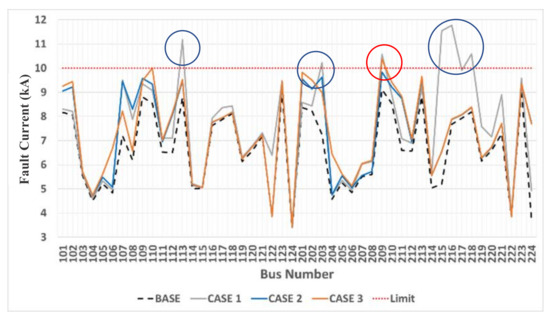
Figure 4.
Fault current analysis using PSS/e ASCC.
Table 4.
Fault current of buses (violated buses only, unit: A).
In Figure 4, the result of Case 1 yields fault currents that exceed 10 kA in the buses of 113, 203, 209, 215, 216, and 218 (blue and red circles). In view of the fault current, the biggest problem of Case 1 is that some of the new transmission lines are constructed on the bus 215, 216, and 218, which have the largest increase in fault currents. It is an obvious result because the fault current level constraint is not considered in the optimization model in Case 1.
On the other hand, any of the fault currents of Case 2 does not exceed the limit of the failure level and the new transmission lines are constructed on the buses 112, 211, and 224 with relatively low increase in fault current.
In Case 3, it can be observed that the fault current at bus 209 exceeds the upper limit as shown in Figure 4 (red circle) and Table 4, and the cause of this problem is due to the linearization of the bus impedance update equation explained in Section 2.2.1. This result can be seen to be due to a rather extreme setting, but we believe that there is always the possibility of this problem occurring in a real system considering the recent circumstances of the power system where the margin between the fault current level and the circuit breakers’ breaking capacity decreases gradually. One thing that should be noted in the result of Case 3 is that the fault current violation happened at bus 209, which is not connected to any of the new transmission lines as shown in Table 3. The reason for this problem is that when the impedance matrix is updated in Case 3 using Equations (6)–(9), the change of the impedance values between other buses that are not connected to the new transmission lines are ignored in order to reduce the calculation time. This problem does not occur in the proposed method (Case 2) because fault current is calculated using exact impedance matrices that reflect the change in the impedance of all buses.
The objective value and the calculation time for each case are shown in Table 5. As shown in the table, Case 2 (the proposed method) takes longer to find the optimal solution than other cases, and the objective function (construction, operation costs, and salvage values) shows that the proposed method is slightly improved compared to Case 3, but the differences are not significant considering the circumstances of the TEP problem. Therefore, the main advantage of the proposed method is that the TEP problem considering the fault current constraint can be solved more precisely by formulating it in MILP form without linearization.
Table 5.
Objective values and computation times.
One last analysis of the proposed method is the impact of the valid inequality on the time to convergence at the optimal solution. Figure 5 shows the results of comparing convergence times with and without using the valid inequality. As shown in the figure, the duality gap converges at 0 in about 267 seconds, but it takes longer than 1000 minutes when the valid inequality is not used. The results of the transmission expansion plan in both cases are exactly the same, and therefore, the effect of the valid inequality is clear.
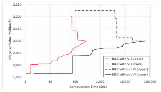
Figure 5.
Impact of the valid inequality on convergence time.
5. Concluding Remarks
In this paper, we propose a new method to solve the TEP problem with more exact consideration of fault current level constraint. In the existing TEP studies, approximation errors occur due to the linearization of the impedance update equation, which is formulated as a nonlinear equation to calculate the fault current of a system. In this paper, we adopt a method of eliminating the approximation error by obtaining the updated impedance matrix directly from the inversion of the admittance matrix using the IMML.
This study also proposes a novel valid inequality method to reduce the computation time to find the optimal solution to the TEP problem with fault current level constraint. The concept of valid inequality is a way of reducing the overall computation time by adding an inequality constraint at every computation step that removes the infeasible region of the optimization problem from the search space. In this paper, the valid inequality is constructed using the characteristic that the fault current in the system generally increases due to the increase of the parallel circuit when new transmission lines are added. As shown in the simulation results, this valid inequality proves to be capable of reducing the overall computation time significantly.
The contribution of this study can be summarized as follows. First, the TEP problem considering the fault current constraint is formulated as a MILP optimization problem without linearization. Second, the convergence of the MILP optimization problem is greatly improved by reducing the feasible area through the valid inequality.
In addition to the TEP problem considering the fault current, the proposed method can be applied to studies on the economical evaluation problems of the newly discussed technologies in solving the fault current problem, such as the optimization of bus separation, the superconducting fault current limiter, and the usage of medium voltage direct current.
Author Contributions
Conceptualization, S.L.; methodology, S.L.; software, S.L.; validation, W.K. and H.K.; formal analysis, H.K.; investigation, H.S.; resources, S.L.; data curation, T.H.K.; writing—original draft preparation, S.L.; writing—review and editing, W.K.; visualization, T.H.K.; supervision, W.K.; project administration, W.K.; funding acquisition, W.K.
Funding
This research was supported by the Human Resources Program in Energy Technology of the Korea Institute of Energy Technology Evaluation and Planning (KETEP) granted financial resource from the Ministry of Trade, Industry & Energy, Republic of Korea (No.20174030201770), and also was supported by Basic Science Research Program through the National Research Foundation of Korea (NRF) funded by the Ministry of Education (NRF 2019R1I1A3A01059931).
Conflicts of Interest
The authors declare no conflict of interest.
Nomenclature
| Indices |
| : Index of years : Index of electricity load blocks : Index of buses : Sub-index of buses applying fault current constraint : Index of generators |
| Sets and Function |
| : Set of all planning years : Set of all buses : Set of buses connected to new line candidates : Set of buses to which fault current constraints are applied : Set of all generators : Set of generators connected to bus : Bus pair of new line candidates between bus and : Set of all electricity load blocks : Fuel cost of generator |
| Variables and Time-varying Parameters |
| : Bus admittance matrix in year : Bus impedance matrix in year : Active power output of generator of load block in year : Active power flow of existing line from bus to of load block in year : Active power flow of new line from bus to of load block in year : Binary variable for on/off status of generator at bus of load block in year : Binary variable for construction status of new transmission line at bus in year : Phase angle of bus of load block in year : Solution to the linear relaxation problem of B&C algorithm at bus in year |
| Fixed Parameters |
| : Maximum fault current at bus : Bus admittance matrix between bus and in base year : Bus impedance matrix between bus and in base year : Impedance of new line candidate between bus and : Construction cost of new line candidate between and : Life span of new line candidate between and : Time duration of load block : Discount rate : Coefficients of the cost function of generator : Active power demand at bus of load block in year , : Maximum/Minimum active power output of generator : Maximum active power transmission limit of existing line between bus and ,: Maximum/Minimum active power transmission limit of new line between bus and : Susceptance of transmission line between bus and : Susceptance of new line candidate between bus and , : Maximum/Minimum voltage angle at bus |
Appendix A. Parameters
The following tables show the parameters of the system used in the simulations.
Table A1.
Transmission line data.
Table A1.
Transmission line data.
| Branch | ID | R (p.u.) | X (p.u.) | Limit (MW) | Branch | ID | R (p.u.) | X (p.u.) | Limit (MW) |
|---|---|---|---|---|---|---|---|---|---|
| 101-102 | 1 | 0.003 | 0.014 | 175 | 201-202 | 1 | 0.003 | 0.014 | 175 |
| 101-103 | 1 | 0.055 | 0.211 | 175 | 201-203 | 1 | 0.055 | 0.211 | 175 |
| 101-105 | 1 | 0.022 | 0.085 | 175 | 201-205 | 1 | 0.022 | 0.085 | 175 |
| 102-104 | 1 | 0.033 | 0.127 | 175 | 202-204 | 1 | 0.033 | 0.127 | 175 |
| 102-106 | 1 | 0.050 | 0.192 | 175 | 202-206 | 1 | 0.050 | 0.192 | 175 |
| 103-109 | 1 | 0.031 | 0.119 | 175 | 203-209 | 1 | 0.031 | 0.119 | 175 |
| 104-109 | 1 | 0.027 | 0.104 | 175 | 204-209 | 1 | 0.027 | 0.104 | 175 |
| 105-110 | 1 | 0.023 | 0.088 | 175 | 205-210 | 1 | 0.023 | 0.088 | 175 |
| 106-110 | 1 | 0.014 | 0.061 | 175 | 206-210 | 1 | 0.014 | 0.061 | 175 |
| 107-108 | 1 | 0.016 | 0.061 | 175 | 207-208 | 1 | 0.016 | 0.061 | 175 |
| 108-109 | 1 | 0.043 | 0.165 | 175 | 208-209 | 1 | 0.043 | 0.165 | 175 |
| 108-110 | 1 | 0.043 | 0.165 | 175 | 208-210 | 1 | 0.043 | 0.165 | 175 |
| 111-113 | 1 | 0.006 | 0.048 | 500 | 211-213 | 1 | 0.006 | 0.048 | 500 |
| 111-114 | 1 | 0.005 | 0.042 | 500 | 211-214 | 1 | 0.005 | 0.042 | 500 |
| 112-113 | 1 | 0.006 | 0.048 | 500 | 212-213 | 1 | 0.006 | 0.048 | 500 |
| 112-123 | 1 | 0.012 | 0.097 | 500 | 212-223 | 1 | 0.012 | 0.097 | 500 |
| 113-123 | 1 | 0.011 | 0.087 | 500 | 213-223 | 1 | 0.011 | 0.087 | 500 |
| 114-116 | 1 | 0.005 | 0.059 | 500 | 214-216 | 1 | 0.005 | 0.059 | 500 |
| 115-121 | 1 | 0.006 | 0.049 | 500 | 215-221 | 1 | 0.006 | 0.049 | 500 |
| 115-124 | 1 | 0.007 | 0.052 | 500 | 215-224 | 1 | 0.007 | 0.052 | 500 |
| 116-117 | 1 | 0.003 | 0.026 | 500 | 216-217 | 1 | 0.003 | 0.026 | 500 |
| 116-119 | 1 | 0.003 | 0.023 | 500 | 216-219 | 1 | 0.003 | 0.023 | 500 |
| 117-118 | 1 | 0.002 | 0.014 | 500 | 217-218 | 1 | 0.002 | 0.014 | 500 |
| 117-122 | 1 | 0.014 | 0.105 | 500 | 217-222 | 1 | 0.014 | 0.105 | 500 |
| 118-121 | 1 | 0.003 | 0.026 | 500 | 218-221 | 1 | 0.003 | 0.026 | 500 |
| 119-120 | 1 | 0.005 | 0.040 | 500 | 219-220 | 1 | 0.005 | 0.040 | 500 |
| 120-123 | 1 | 0.003 | 0.022 | 500 | 220-223 | 1 | 0.003 | 0.022 | 500 |
| 107-203 | 1 | 0.042 | 0.161 | 175 |
Table A2.
Transformer data.
Table A2.
Transformer data.
| Branch | R (p.u.) | X (p.u.) | Limit (MW) | Tr | R (p.u.) | X (p.u.) | Limit (MW) |
|---|---|---|---|---|---|---|---|
| 103-124 | 0.002 | 0.09 | 400 | 203-224 | 0.002 | 0.09 | 400 |
| 109-111 | 0.002 | 0.09 | 400 | 209-211 | 0.002 | 0.09 | 400 |
| 109-112 | 0.002 | 0.09 | 400 | 209-212 | 0.002 | 0.09 | 400 |
| 110-111 | 0.002 | 0.09 | 400 | 210-211 | 0.002 | 0.09 | 400 |
| 110-112 | 0.002 | 0.09 | 400 | 210-212 | 0.002 | 0.09 | 400 |
Table A3.
New line data.
Table A3.
New line data.
| Branch | R (p.u.) | X (p.u.) | Limit (MW) | Investment Cost (Million $) | Life (year) |
|---|---|---|---|---|---|
| 102-201 | 0.090 | 0.346 | 175 | 90,000,000 | 30 |
| 106-204 | 0.072 | 0.276 | 175 | 72,000,000 | 30 |
| 107-203 | 0.042 | 0.161 | 175 | 42,000,000 | 30 |
| 107-108 | 0.016 | 0.061 | 175 | 16,000,000 | 30 |
| 112-224 | 0.011 | 0.089 | 500 | 120,000,000 | 30 |
| 113-215 | 0.010 | 0.075 | 500 | 78,000,000 | 30 |
| 113-217 | 0.042 | 0.161 | 175 | 42,000,000 | 30 |
| 115-116 | 0.002 | 0.017 | 500 | 18,000,000 | 30 |
| 115-121 | 0.006 | 0.049 | 500 | 51,000,000 | 30 |
| 116-117 | 0.003 | 0.026 | 500 | 27,000,000 | 30 |
| 118-121 | 0.003 | 0.026 | 500 | 27,000,000 | 30 |
| 119-120 | 0.005 | 0.040 | 500 | 41,250,000 | 30 |
| 120-123 | 0.003 | 0.022 | 500 | 22,500,000 | 30 |
| 121-122 | 0.009 | 0.068 | 500 | 70,500,000 | 30 |
| 122-218 | 0.009 | 0.068 | 500 | 76,500,000 | 30 |
| 123-217 | 0.010 | 0.074 | 500 | 76,500,000 | 30 |
| 203-209 | 0.031 | 0.119 | 175 | 31,000,000 | 30 |
| 207-208 | 0.016 | 0.061 | 175 | 16,000,000 | 30 |
| 215-216 | 0.002 | 0.017 | 500 | 18,000,000 | 30 |
| 215-221 | 0.006 | 0.049 | 500 | 51,000,000 | 30 |
| 218-221 | 0.003 | 0.026 | 500 | 27,000,000 | 30 |
| 219-220 | 0.005 | 0.040 | 500 | 41,250,000 | 30 |
| 220-223 | 0.003 | 0.022 | 500 | 22,500,000 | 30 |
| 221-222 | 0.009 | 0.068 | 500 | 70,500,000 | 30 |
| 211-224 | 0.006 | 0.046 | 500 | 49,500,000 | 30 |
Table A4.
Generator data.
Table A4.
Generator data.
| Bus ID | Pmax (MW) | Pmin (MW) | Bg ($/MWh) | Cg ($/h) | Xd″ (p.u) | Bus ID | Pmax (MW) | Pmin (MW) | Bg ($/MWh) | Cg ($/h) | Xd″ (p.u) |
|---|---|---|---|---|---|---|---|---|---|---|---|
| 101 | 192 | 154 | 52 | 1220 | 0.19 | 201 | 192 | 154 | 42 | 976 | 0.19 |
| 102 | 192 | 154 | 52 | 1220 | 0.19 | 202 | 192 | 154 | 42 | 976 | 0.19 |
| 107 | 300 | 70 | 78 | 13,152 | 0.13 | 207 | 300 | 70 | 62 | 10,521 | 0.13 |
| 113 | 591 | 352 | 4 | 281 | 0.06 | 213 | 591 | 352 | 3 | 225 | 0.06 |
| 115 | 215 | 152 | 71 | 9116 | 0.17 | 215 | 215 | 152 | 56 | 7293 | 0.17 |
| 116 | 155 | 44 | 113 | 7810 | 0.24 | 216 | 155 | 44 | 91 | 6278 | 0.24 |
| 118 | 400 | 244 | 20 | 3848 | 0.12 | 218 | 400 | 244 | 17 | 3078 | 0.12 |
| 121 | 400 | 244 | 24 | 3452 | 0.12 | 221 | 400 | 244 | 19 | 2762 | 0.12 |
| 122 | 300 | 122 | 129 | 2778 | 0.12 | 222 | 300 | 122 | 103 | 2222 | 0.12 |
| 123 | 660 | 562 | 5 | 947 | 0.06 | 223 | 660 | 562 | 4 | 758 | 0.06 |
Table A5.
Peak load data (MW).
Table A5.
Peak load data (MW).
| Bus ID | kV | Peak Load | Bus ID | kV | Peak Load | Bus ID | kV | Peak Load | Bus ID | kV | Peak Load |
|---|---|---|---|---|---|---|---|---|---|---|---|
| 101 | 138 | 92 | 111 | 230 | 225 | 201 | 138 | 46 | 211 | 230 | 113 |
| 102 | 138 | 82 | 112 | 230 | 167 | 202 | 138 | 41 | 212 | 230 | 84 |
| 103 | 138 | 153 | 113 | 230 | 225 | 203 | 138 | 77 | 213 | 230 | 113 |
| 104 | 138 | 63 | 114 | 230 | 165 | 204 | 138 | 31 | 214 | 230 | 82 |
| 105 | 138 | 60 | 115 | 230 | 269 | 205 | 138 | 30 | 215 | 230 | 135 |
| 106 | 138 | 116 | 116 | 230 | 85 | 206 | 138 | 58 | 216 | 230 | 43 |
| 107 | 138 | 106 | 118 | 230 | 283 | 207 | 138 | 53 | 218 | 230 | 142 |
| 108 | 138 | 145 | 119 | 230 | 154 | 208 | 138 | 73 | 219 | 230 | 77 |
| 109 | 138 | 149 | 120 | 230 | 109 | 209 | 138 | 74 | 220 | 230 | 54 |
| 110 | 138 | 166 | 210 | 138 | 83 |
References
- Sarmiento, H.G.; Castellanos, R.; Pampin, G.; Tovar, C.; Naude, J. An example in controlling short circuit levels in a large metropolitan area. In Proceedings of the 2003 IEEE Power Engineering Society General Meeting (IEEE Cat. No.03CH37491), Toronto, ON, Canada, 13–17 July 2003; Volume 2, pp. 589–594. [Google Scholar]
- Vovos, P.N.; Bialek, J.W. Direct incorporation of fault level constraints in optimal power flow as a tool for network capacity analysis. IEEE Trans. Power Syst. 2005, 20, 2125–2134. [Google Scholar] [CrossRef]
- Moon, G.; Wi, Y.; Lee, K.; Joo, S. Fault Current Constrained Decentralized Optimal Power Flow Incorporating Superconducting Fault Current Limiter (SFCL). IEEE Trans. Appl. Supercond. 2011, 21, 2157–2160. [Google Scholar] [CrossRef]
- Vovos, P.N.; Song, H.; Cho, K.; Kim, T. A network reconfiguration algorithm for the reduction of expected fault currents. In Proceedings of the 2013 IEEE Power Energy Society General Meeting, Vancouver, BC, Canada, 21–25 July 2013; pp. 1–5. [Google Scholar]
- Ngoc, P.T.; Singh, J.G. Short circuit current level reduction in power system by optimal placement of fault current limiter. Int. Trans. Electr. Energy Syst. 2017, 27, 2457. [Google Scholar] [CrossRef]
- Moon, G.; Lee, J.; Joo, S. Integrated Generation Capacity and Transmission Network Expansion Planning With Superconducting Fault Current Limiter (SFCL). IEEE Trans. Appl. Supercond. 2013, 23, 5000510. [Google Scholar] [CrossRef]
- Teimourzadeh, S.; Aminifar, F. MILP Formulation for Transmission Expansion Planning With Short-Circuit Level Constraints. IEEE Trans. Power Syst. 2016, 31, 3109–3118. [Google Scholar] [CrossRef]
- Gharibpour, H.; Aminifar, F.; Bashi, M.H. Short-circuit-constrained transmission expansion planning with bus splitting flexibility. IET Gener. Transm. Distrib. 2017, 12, 217–226. [Google Scholar] [CrossRef]
- Ghanaatian, M.; Lotfifard, S. Sparsity-Based Short-Circuit Analysis of Power Distribution Systems With Inverter Interfaced Distributed Generators. IEEE Trans. Power Syst. 2019, 34, 4857–4868. [Google Scholar] [CrossRef]
- Džafić, I.; Pal, B.C.; Gilles, M.; Henselmeyer, S. Generalized π Fortescue Equivalent Admittance Matrix Approach to Power Flow Solution. IEEE Trans. Power Syst. 2014, 29, 193–202. [Google Scholar] [CrossRef]
- Grainger, J.J.; Stevenson, W.D. Power System Analysis; Mcgrawhill: New York, NY, USA, 2003. [Google Scholar]
- Alsac, O.; Stott, B.; Tinney, W.F. Sparsity-Oriented Compensation Methods for Modified Network Solutions. IEEE Trans. Power Appar. Syst. 1983, 102, 1050–1060. [Google Scholar] [CrossRef]
- Glover, J.D.; Sarma, M.S.; Overbye, T.J. Power System Analysis and Design, 5th ed.; Cengage Learning: Boston, MA, USA, 2012. [Google Scholar]
- GAMS Solvers. Available online: https://www.gams.com/latest/docs/S_MAIN.html. (accessed on 17 January 2017).
- Gendreau, M.; Laporte, G.; Semet, F. A branch-and-cut algorithm for the undirected selective traveling salesman problem. Networks 1998, 32, 263–273. [Google Scholar] [CrossRef]
- Ostrowski, J.; Anjos, M.F.; Vannelli, A. Tight Mixed Integer Linear Programming Formulations for the Unit Commitment Problem. IEEE Trans. Power Syst. 2012, 27, 39–46. [Google Scholar] [CrossRef]
- Brimberg, J.; Hansen, P.; Lin, K.-W.; Mladenović, N.; Breton, M. An Oil Pipeline Design Problem. Oper. Res. 2003, 51, 228–239. [Google Scholar] [CrossRef]
- Mitchell, J.E. Branch-and-cut algorithms for combinatorial optimization problems. Handb. Appl. Optim. 2002, 1, 65–77. [Google Scholar]
- Grigg, C.; Wong, P.; Albrecht, P.; Allan, R.; Bhavaraju, M.; Billinton, R.; Li, W. The IEEE Reliability Test System-1996. A report prepared by the Reliability Test System Task Force of the Application of Probability Methods Subcommittee. IEEE Trans. Power Syst. 1999, 14, 1010–1020. [Google Scholar] [CrossRef]
- Rosenthal, R.E. GAMS-A User’s Guide; GAMS Develop. Corpor.: Washington, DC, USA, 2016. [Google Scholar]
- PSS®E Homepage. Available online: New.siemens.com/global/en/products/energy/services/transmission-distribution-smart-grid/consulting-and-planning/pss-software/pss-e.html (accessed on 20 March 2019).
© 2019 by the authors. Licensee MDPI, Basel, Switzerland. This article is an open access article distributed under the terms and conditions of the Creative Commons Attribution (CC BY) license (http://creativecommons.org/licenses/by/4.0/).