1. Introduction
Reservoir simulation is a powerful tool to predict reservoir performance under different operating conditions, however, when it comes to fractured wells, it requires detailed knowledge of induced fractures. Routinely, well testing and long-term rate-transient analysis (RTA) are used for post-fracture analysis to determine fracture properties [
1,
2]. Recent advances in field data acquisition and development of powerful data analytic techniques promise new venues for unlocking fracture properties such as fracture conductivity and complexity of induced fracture networks by analysis of flowback data if a good physical model for flowback is available. Flowback data is the earliest part of production data that operators may acquire to determine fracture properties for building reservoir models and assess the stimulation design.
The first attempt to quantitively analyze flowback data uses a single-phase reciprocal productivity Index (RPI) procedure [
3]. This method provides an estimation of the effective permeability-thickness, apparent fracture half-length or effective wellbore radius for vertical wells. The model is derived based on the bi-wing planar fracture geometries and assumes that fracture volume does not change during flowback. Flowback production time in shale wells is divided into three periods: (1) the pre-breakthrough water dominated region, (2) the transition region, and (3) the post-breakthrough hydrocarbon dominated region [
4]. The authors developed a single-phase flowback model for the first period only and assumed a linear correlation between rate-normalized pressure and material balance flowrate to calculate total storage coefficients and effective fracture permeability. A semi-analytical model for flowback in tight oil reservoirs uses the concept of a dynamic drainage area (DDA) to capture the transient behaviors [
5]. A bi-wing planar fracture is assumed in the model. However, due to the presence of natural fractures in the formation and their interaction with advancing hydraulic fractures, the geometry of induced fractures can be very complicated [
6]. The outcrop of cross-cutting joints found in the Marcellus shale exposed in Oatka Creek also shows well-developed natural fracture systems [
7]. To accommodate the reactivation of pre-existing natural fractures, they defined an enhanced fracture region (EFR) along the primary fracture, inside which the permeability is enhanced. However, this approach indicates that overall permeability is enhanced in the direction perpendicular to the primary fracture, which misleads the true directionality of fracture permeability in complex fracture networks [
8]. A complex fracture network is desirable from the design perspective as it increases the effective surface area of the wellbore and enable more-efficient linear flow to predominate over the radial flow. Production from reservoirs with complex fracture networks is often modeled by a numerical simulator, which can be computationally expensive for use in inverse analyses, unless some meshless methods are utilized for flow through fractures [
9]. Most available flowback models incorporate fracture closure by using constant fracture compressibility for wells with bi-wing planar fractures [
4,
5,
8,
10]. However, the outcome can be misleading for two main reasons: (1) compressibility of propped fracture is expected to evolve with effective pressure based on the analytical solution for compliance of proppant beds. Especially during early flowback, rapid pressure drawdown may lead to significant decrease in fracture compressibility. Flowback analysis based on constant compressibility will overestimate the fracture storage capacity at the end of flowback. (2) Fracture width is decreasing from the wellbore to the tip, knowing that fracture compressibility is a function of proppant density, we do not expect that fracture compressibility remains constant. This assumption can introduce misleading impacts on determining fracture properties. To incorporate compressibility changes over time, we initially proposed analytical solutions for single and two-phase water–oil flowback using eigenfunction expansion methods. Then, we develop a semi-analytical procedure to incorporate variations of fracture width and fracture compressibility along the fracture, which can be utilized for complex fracture networks and long-planar fractures. We also proposed a two-phase oil-water flowback solution with matrix oil influx for wells with bi-wing planar fractures, which can be applied to formations without significant natural fractures. The proposed model is verified against numerical simulations implemented in COMSOL Multiphysics (COMSOL, Burlington, Massachusetts, USA) Multiphysics and CMG (Computer Modelling Group LTD., Calgary, Alberta, Canada). The goals of this paper are set to (1) provide a quick and accurate direct flowback model for fluid flow through the fracture network, (2) investigate the influence of non-uniform fracture closure and variable fracture compressibility on flowback characteristics.
2. Governing Equations for Flowback Models
Flowback from shale oil wells often initially show only a typical single-phase region. Assuming there is no matrix flow, the dimensionless form of the governing equation for 1D single-phase flowback is given by
where dimensionless variables are defined as
where
is fluid pressure along the fracture,
is the initial fracture pressure,
is the average pressure in the fracture,
is the length of the fracture segment,
is porosity,
is water viscosity,
is fracture permeability,
is dimensionless fracture width which is defined as
, x is the coordinate along the fracture direction.
is the total compressibility which is the summation of fracture compressibility
and water compressibility
, which are defined as follows
In the case of wells with an extended shut-in period, a small amount of oil may enter the fracture network. The following assumptions should be considered to develop the two-phase oil–water model: (1) capillary pressure is neglected inside the fractures, (2) oil and water are both incompressible, and (3) no matrix flow is considered. The average saturation of the fracture domain does not change due to the assumption of incompressible fluids as the coefficients of
terms collapse to zero in the two-phase governing equation. The mass balance equation for the fracture system is the same as Equation (1), except the pseudo-time is defined differently as
where
is the summation of
and
, which are oil mobility and water mobility defined as
and
. The straight-line relative permeability model is used for fractures in this study i.e.,
where
is water saturation. Detailed derivation of governing equations for a two-phase flow without matrix influx is provided in
Appendix B.
During the flowback period, initially, water production dominates (region 1) which is gradually replaced by oil production (region 3) after oil breakthrough the fracture as shown schematically in
Figure 1. Since the permeability of shale reservoirs is extremely low, no matrix flow from the reservoir is considered for early-time flowback. As a result, the proposed flowback model will be restricted to region 1. Due to the extremely small pore diameter of the shale formation, the large capillary effect is expected. Therefore, breakthrough pressure can be much lower than initial reservoir pressure, which makes the closed-chamber solution works for an extended period of time.
Even though the solution developed by assuming no matrix influx is accurate in early flowback periods, it cannot predict flowrate accurately for the late flowback period after a significant amount of oil enters the fracture network. To test the applicability of the above-mentioned model without considering matrix flow, we proposed another solution that can consider matrix flow but only limited to wells with bi-wing planar fractures. In the fracture governing equation, the matrix influx is considered as a source term, which is given by
where
The matrix oil velocity
is calculated from the matrix governing equation
where
where
represents matrix pressure,
D represents the length of stimulated reservoir volume (SRV) or half of the fracture spacing for multi-stage hydraulic fractures in horizontal wells. Although
the term is canceled out, water saturation inside the fracture should be updated from the volume balance equation to update the relative permeability values.
3. Analytical Solution of Governing Equations
The eigenfunction expansion methods are used to solve the diffusivity equation with time-dependent boundary conditions. The analytical solutions of Equation (1) can be classified into two cases based on the boundary conditions. One case is variable pressure boundary conditions at both fractures’ ends and the other case is variable pressure at one end and no flow at the other end. Detailed derivation of the solution is provided in
Appendix A. Initial condition of Equation (1) for is given by
First, we present the solution for variable pressure boundary conditions at both ends of the fracture without matrix influx, time dependent pressure boundary conditions are prescribed at both ends as
Using an eigenfunction expansion for the solution
as shown in
Appendix A, analytical solution of Equation (1) with two Dirichlet boundary conditions are given by
where
is the Fourier series obtained from the initial conditions,
is the term that accounts for the time derivative of the two Dirichlet boundary conditions,
is the eigenvalue:
In the single-phase solution, water rate can be evaluated by taking derivative of Equation (21) with respect to x as
Similarly, in the two-phase solution, the total flow rate at the inlet and outlet are
For solution with variable pressure boundary condition at one end and no-flow boundary at the other end without matrix influx, time-dependent pressure boundary conditions are prescribed at both ends as
Using an eigenfunction expansion for the solution
as shown in
Appendix A, the analytical solution of Equation (1) with one Dirichlet boundary condition and one Neumann boundary condition is
where
In the single-phase solution, water rate can be evaluated by taking the derivative of pressure, i.e.,
In the two-phase solution, total flow rate can be evaluated as
For two-phase flowback with matrix influx, the concept of pseudo-pressure is used to capture the saturation change inside the fracture. Initial condition of Equation (10) for fracture flow is given by
The time-dependent pressure boundary conditions are prescribed at both ends as
Using the eigenfunction expansion for homogenized pseudo-pressure, the analytical solution of Equation (10) will be
where
Taking the derivative of the pseudo-pressure, the total flow rate at the wellbore can be evaluated as
Water rate and oil rate can be evaluated as,
Since the source term in Equation (10) is obtained by solving the matrix flow equation, matrix oil velocity also needs to be updated. The computational cost of the solution is O(M), where M is the number of total segments. To balance the accuracy and computational costs, we divided each half of the fracture into four segments
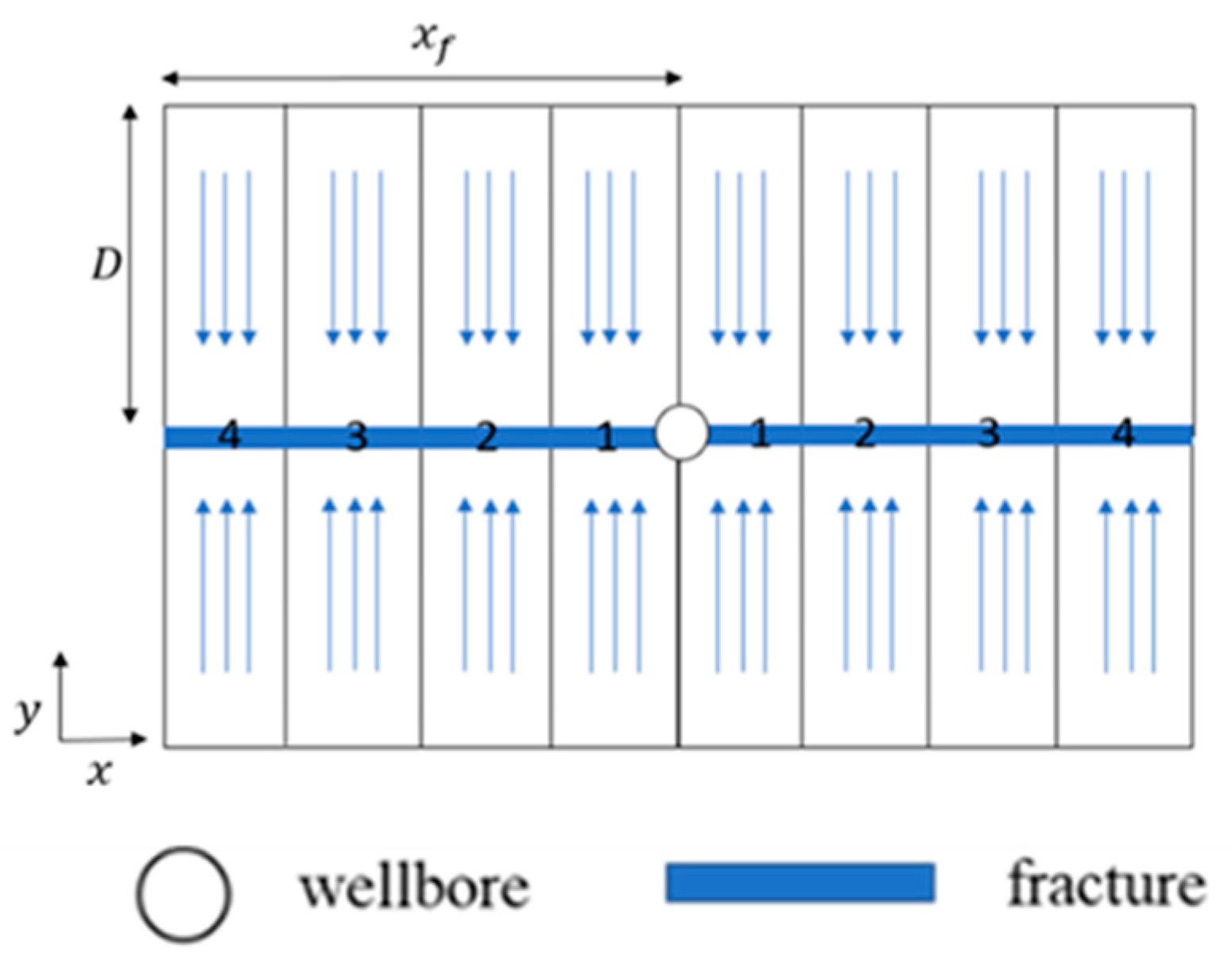
Figure 2 shows hydraulic fractures in a given stimulated reservoir volume (SRV), which is assumed to have a rectangular shape. Matrix oil flux is calculated separately for the four fracture segments. Initial and boundary conditions of the matrix oil flow equation is given by
where
represents the average pressure at segment
k. The analytical solution of Equation (14) is given by
Average water saturation in the fracture segment k is determined using volume balance as
where
is the initial water saturation, dt is time step and
is the volume of the fracture segment at the current time.
and
is the inflow and outflow water rates, respectively. The continuous water saturation profile inside the fracture is approximated by a second-order polynomial interpolation between nodal saturations
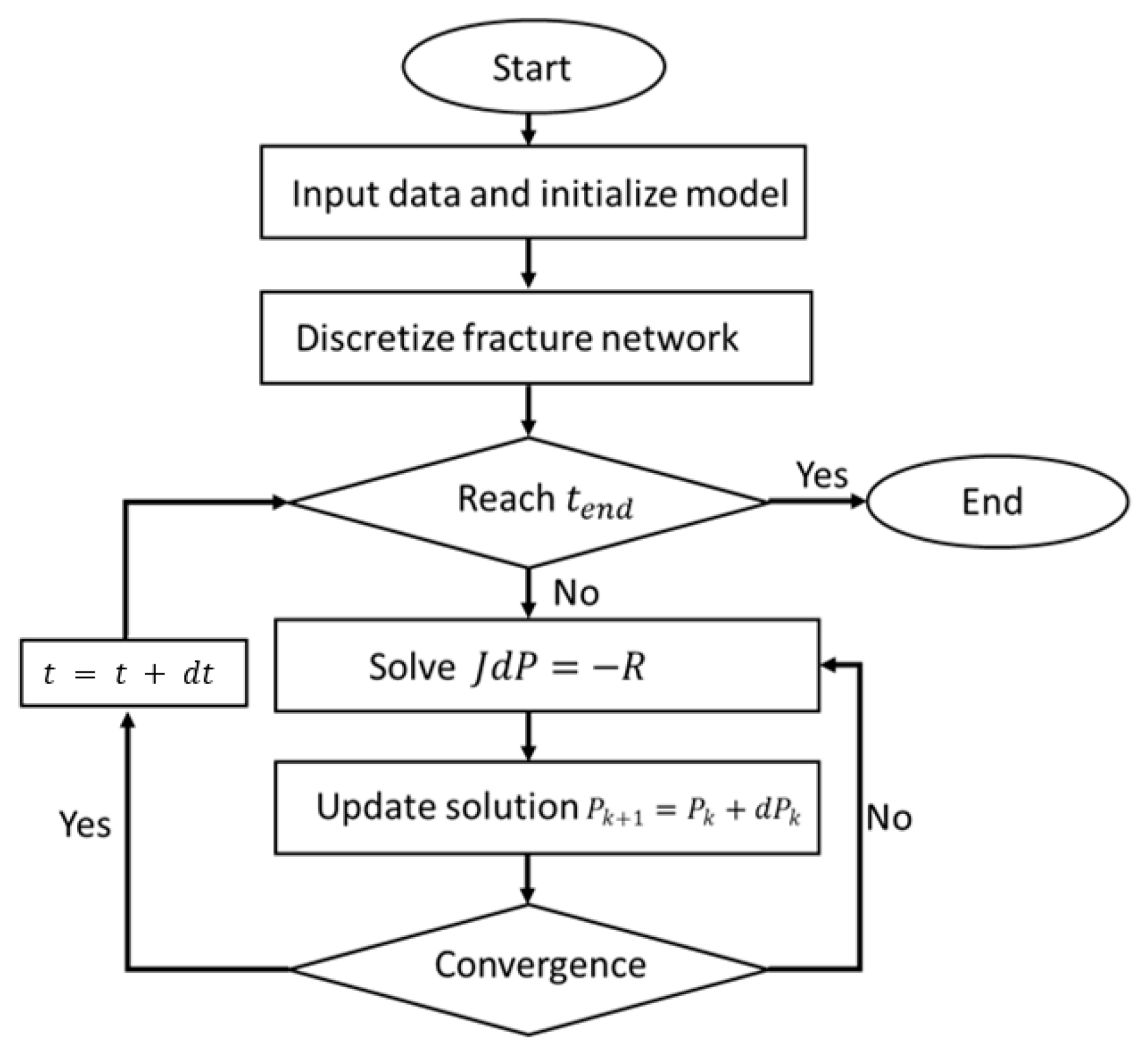
The two-phase flowback solution with matrix oil influx can be described as following:
For the first time step, the average saturation in each segment is equal to initial water saturation (). Solve Equation (10) by Equations (40) and (44) assuming no oil influx at the initial time () and calculate average fracture pressure for each fracture segment.
Based on , calculate average oil influx using Equation (51).
For the second time step, update oil rate calculated from step 2 in Equation (10) and solve it again. Average water saturation for each segment is calculated from the material balance Equation (52). Update pressure and repeat steps 2–3 till reaching the end of the simulation time.
We also show the workflow of the solution in
Figure 3.
The analytical solutions presented in this section is only applicable to a single fracture segment. however, fractures may exist in the form of complex networks. In the following sections, we will show how we can discretize the complex networks and solve the systems of equations simultaneously for the whole system.
4. Fractal Fracture Network and Fracture Discretization
Two different fracture network geometries are considered in this study: tree-shape fracture networks and orthogonal fracture networks. Fracture re-initiation at the intersection with natural fractures is a possible branching mechanism during hydraulic fracturing [
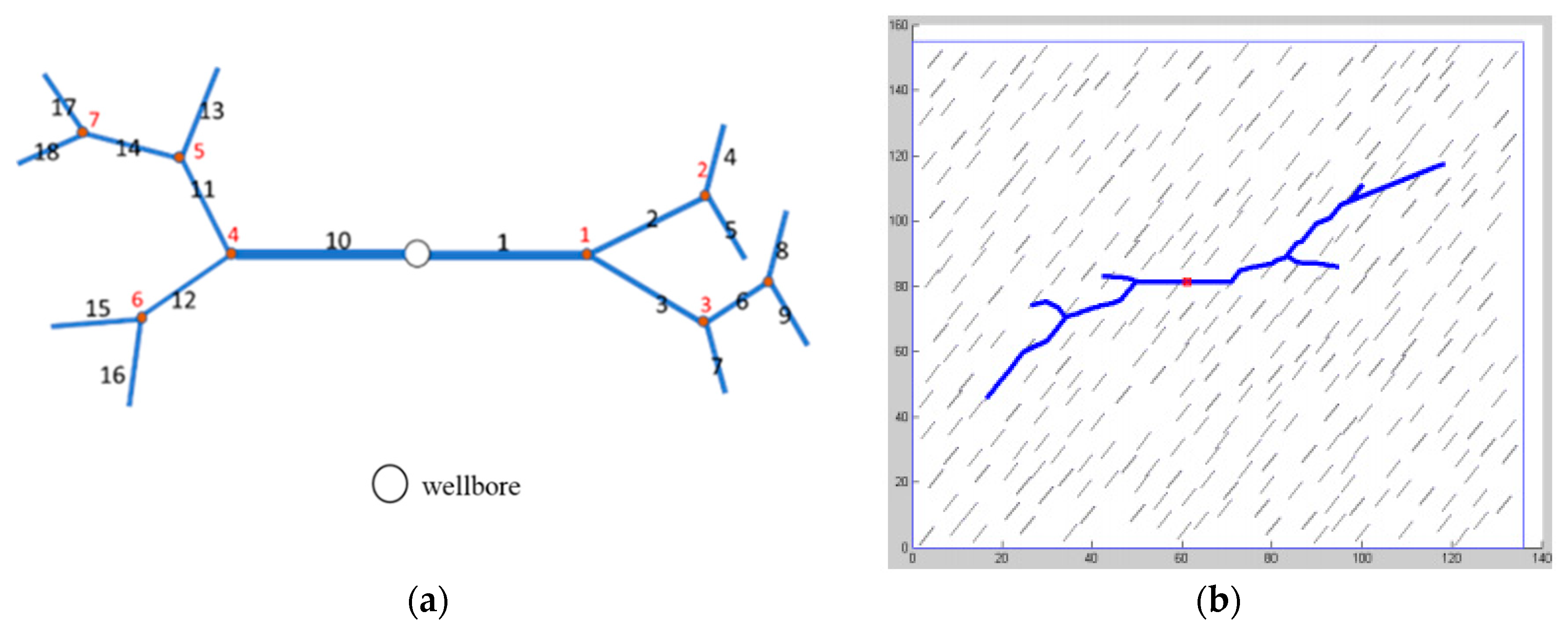
11]. Tree-shape fracture networks are commonly found as shown in
Figure 4b from simulation results. Researchers used a neural network model to process microseismic data to estimate fracture geometry and also believe that, the fracture network of multiple fractured horizontal wells in highly brittle shale formation is usually tree-shaped [
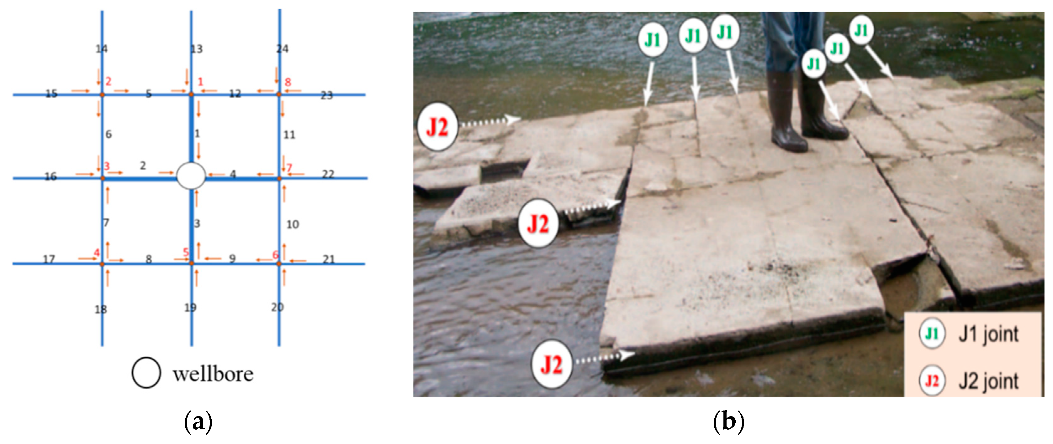
12]. An orthogonal fracture network is another common situation in complex fracture networks. In naturally fractured formations, if the joint sets are orthogonal to each other, like the situation in Marcellus Shale [
11], induced hydraulic fractures may likely form an orthogonal mosaic network by activating natural fractures as shown in
Figure 4b.
Fracture discretization is the first step to simplify calculations. Fracture networks can be divided into multiple segments and nodes as illustrated in
Figure 4a and
Figure 5a for tree-shape and orthogonal fractures, respectively. The tree-shape network is divided into 18 segments and 8 nodes. The orthogonal fracture network is divided into 24 segments and eight nodes. It is worth noting that in the case of symmetric tree-shape or symmetric orthogonal fracture networks, one may take advantage of the symmetry and reduce the number of nodes and segments to reduce the computational costs.
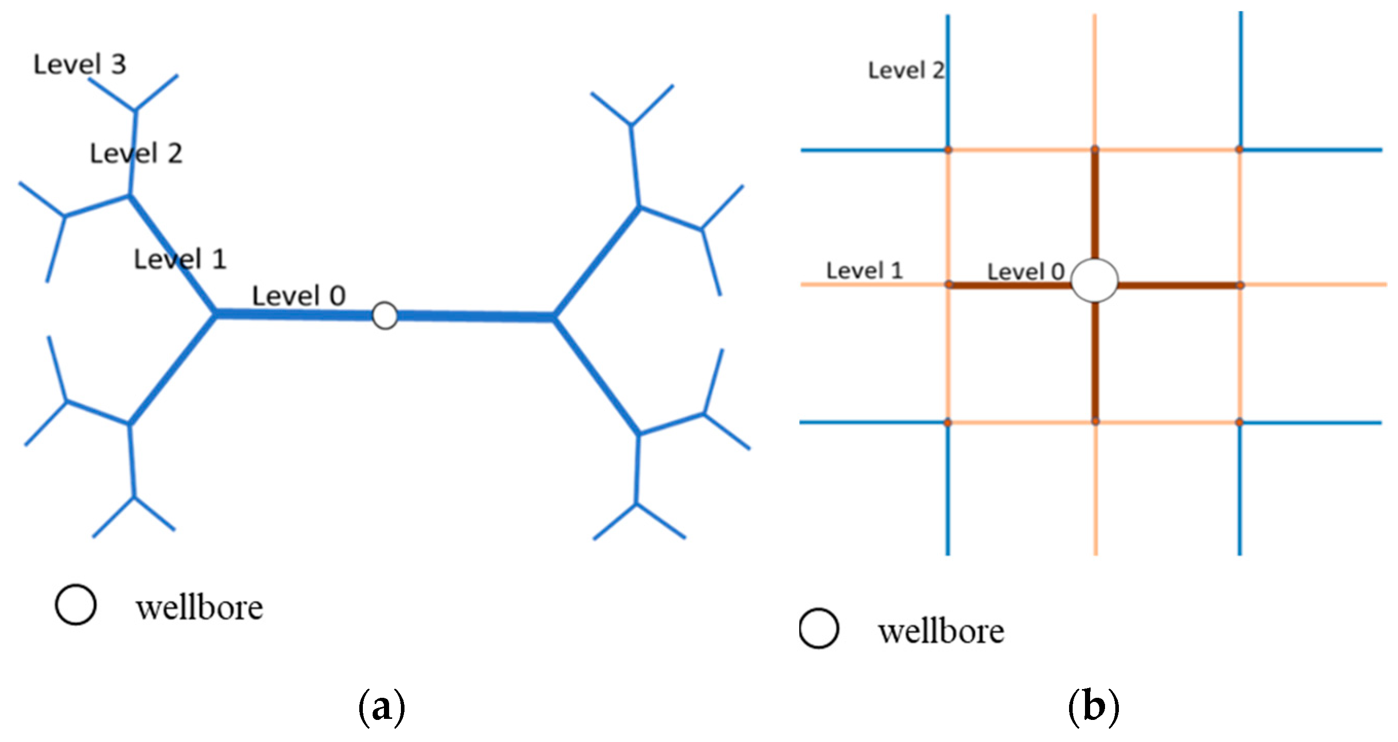
To generalize fracture networks, tree-shape fracture networks and orthogonal fracture networks can be synthesized using fractal theory as shown in
Figure 6. In a tree-shape fracture network (
Figure 4a), each fracture segment can be modeled with segment length
, width
and compressibility
, where index i denotes the fracture-segment generation level. The oldest or initial segment is obviously near the well (
i = 0).
The structure and properties of the network can be characterized by fractional changes after each generation based on fractal theory i.e.,
In orthogonal fracture networks, the width of the fracture segments decreases with the distance from the wellbore, which can be easily verified by stress analysis [
13]. The structure and properties of the orthogonal network can also be characterized by fractional reduction after each intersection away from the wellbore as shown in Equations (53) and (54). The compressibility of the activated natural fractures which are labeled with level number larger than 0 in
Figure 6 because width reduction also indicates less layers of proppants. The permeability of the activated natural fractures is assumed to be the same.
For the case of long planar fractures, non-uniform fracture width and non-uniform fracture closure can be simulated by discretizing the fracture into several segments as shown in
Figure 7. The width of fractures decreases away from the wellbore. For each segment, the width of the segment can be set with an average value based on experience or hydraulic fracturing simulation results [
13,
14,
15].
To model fracture closure more accurately, understanding of fracture properties is of great importance. Current models for flowback analysis assume that fracture properties, such as fracture permeability and fracture compressibility, do not change over time. In this paper, we will estimate the evolution of these properties with time-based on the mechanical interaction between the formation rock and proppants. For propped fractures, compressibility is contributed by two components: fracture aperture changes and fracture porosity change [
16], i.e.,
To incorporate fracture aperture changes during flowback, we adopt the analytical solution for normal compliance of the propped fracture [
17]. Assuming there is no slippage between the particles and deformation between the proppant particles is elastic, the compressibility of the fracture due to its width change
can be obtained by
where
n is the number of proppant layers,
is the effective normal stress on proppants,
and
are the Young’s Moduli of the formation and proppants, respectively.
and
are Poisson’s ratios of the formation rock and proppant particles, respectively. We adopt a model to estimate the porosity of the proppants pack [
18], that can be simplified as
where
is the initial porosity of the proppant pack,
is a constant depending on the packing structure. Hence, porosity compressibility is estimated from the model by assuming that fracture porosity is equal to the proppant pack as,
Permeability can also be modeled as in [
18]
Thus, total fracture compressibility can be expressed as a function of effective normal stress, proppant properties and mechanical properties of the formation,
In this study, we compare the flowback response for fracture propped with two kinds of proppants, sand, and ceramics whose properties are shown in
Table 1. In comparison to sand, ceramics have a higher strength and is less compressible. Young’s modulus and Poisson’s ratio of the formation used in this study is assumed to be 25 Gpa and 0.27, respectively. The size of the proppants used in this study is close to 40–70 mesh, we consider an average radius of the proppant is 0.3 mm in the analytical model on fracture compressibility. However, our proposed model is not limited to a specific mesh size and the same procedure can be applied for different proppant mesh sizes.
It is worth noticing that in the case with partial proppants coverage, a considerably high fracture compressibility can be used to model the rapid closure of the unpropped part of the fracture.
Upon discretization of the complex fracture networks, the analytical solution for each discretized fracture segment will be solved simultaneously. The next section is dedicated to introducing the numerical technique we utilized for the semi-analytical approach.
6. Results and Discussions
To test the accuracy of the proposed semi-analytical model for flowback analysis of the wells completed in shale oil reservoirs, several examples are generated and compared with results from full-fledged numerical simulations with COMSOL Multiphysics and CMG for the two different topologies for fracture networks used in this study. In COMSOL Multiphysics, the diffusivity equation is solved by the built-in two-phase Darcy’s flow module using the finite element methods, which allows the generation of fracture networks with non-orthogonal topology. About 3000 quadratic elements is used to solve the two-dimensional, two-phase oil–water flow in both fractal tree-shape and orthogonal fracture networks without matrix influx. Only half of the fracture is modeled due to the symmetry of the problem. A pressure boundary condition is applied at the mouth of the fracture. In CMG, only a quarter of the reservoir is modeled due to the symmetry of the problem with finite difference methods. About 10,000 elements including fracture elements and matrix elements are used to model the two-phase flow with matrix influx. A layer of the elements represents one-half of the fracture, which has higher permeability in comparison to the other elements. The element at the end of the fracture elements is representing the well. The H-adaptive mesh is adopted i.e., elements are coarsening as moving from the fracture to the distant reservoir.
A summary of the reservoir and fracture network properties used in our examples is provided in
Table 2. The fracture networks shown in
Figure 4 are used for validation purposes. For the orthogonal fracture network, starting from the wellbore, fractures’ width and permeability reduce 25% after each intersection away from the wellbore. For the tree-shape fracture network, fracture segments’ width reduces 50% after each generation as indicated by earlier geomechanical simulations [
13]. In this study, we presumed a smooth pressure drawdown characteristic at the wellbore during early flowback using the below form function,
where
a is the drawdown coefficient with the value of 100,000 for our validation example,
t is time (in seconds).
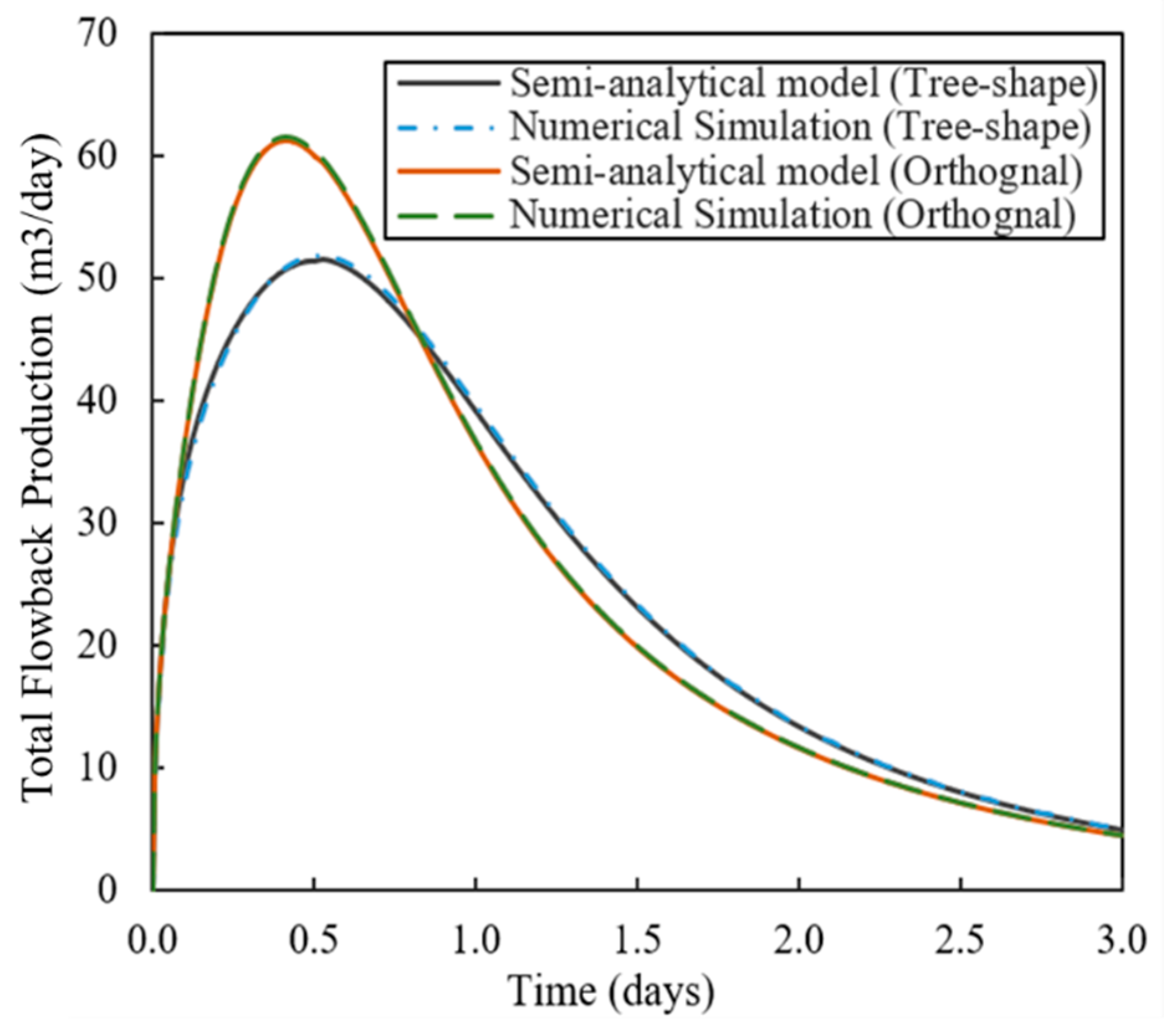
A good match for total production between the semi-analytical model and commercial numerical simulations has been obtained to verify the proposed analytical solution as shown in
Figure 9. The computational cost of the semi-analytical model in MATLAB (MathWorks, Natick, MA, USA) and the numerical model in COMSOL Multiphysics is compared in
Figure 10. In order to examine the influence of the fracture network topology on the flowback behavior, we compare flowback rate from a tree-shape and an orthogonal network fractures sets with the same total length and total fracture volume as shown in
Table 2. The reader may notice that the flowrate in the orthogonal fracture network reaches a higher peak in flowrate in comparison to tree-shape fracture but declines faster. The probable reason for this phenomenon is higher conductivity in the orthogonal fracture set in comparison to the tree-shape network with the same volume and length. Different flowback behaviors in the two fracture networks indicate that flowback analysis based on the material balance could be misleading since it cannot capture the effect of the network topology.
For the purpose of doing a sensitivity analysis, we considered the cases described earlier as the base case, and only change a key parameter each time with respect to the base case.
The total fracture volume of the fracture network can be calculated using the length of fracture segments and their corresponding widths. Since it is not realistic to assign a single width to all fractures and on the other hand, it would be computationally very expensive to consider a variable width along all each fracture segment, we use a simplifying hypothesis consistent with geomechanical analyses. We are presuming a value for the width of the fracture segment connected to the well and then assuming a fixed ratio for the fracture width reduction at each intersection away from the wellbore. Therefore, we can investigate the effect of the fracture width distribution by changing the maximum width at the wellbore and the ratio of width changes. In general, increasing fracture width or its length increases the volume inside the fracture network. The influence of the fracture volume on flowback looks similar in both fracture networks.
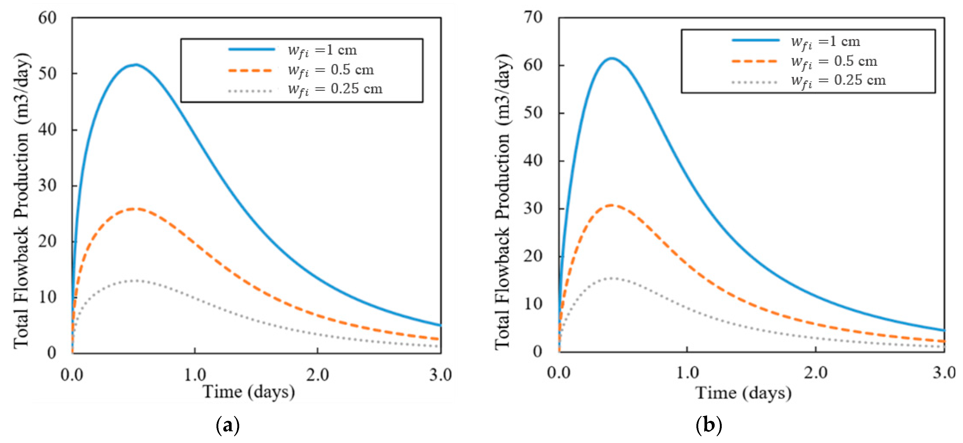
6.1. Flowback Responses with Different Fracture Volume
Figure 11 compares the flowback rate for different maximum fracture width (different
) in tree-shape networks and orthogonal networks. We can see that in both cases, the flowback rate is nearly proportional to the maximum fracture width (otherwise known as average fracture width). It is also notable that the peak time for the flowrate does not shift with changes in the maximum fracture width as the topology of the fracture network remains the same. In shale gas wells due to nonlaminar effects, this observation may not be necessarily true.
Figure 12 compares the flowback rate for different ratios of the fracture width reduction (different
). The result shows that the flowback rate looks similar initially during the transient flow period. Though after a while, the flowrates slightly increase with higher
. We also noticed that changing
shifts the peak time for the flowback rate. The occurrence of peak flowrate delays slightly with higher value of
. A similar phenomenon may also happen with the increase of the total fracture length. Since several parameters affect the flowback behaviors together, the inverse analysis using the proposed model can be non-unique. Hence, constraining one of these values would be helpful to reach a unique fracture network geometry during inverse analyses. For instance, knowledge of micro-seismic data and injection volume can be helpful for estimating the total fracture volume. Fracture width reduction can also be estimated from a coupled analysis of the hydraulic fracturing treatment. Proppant concentration, fracking fluid viscosity, viscosity degradation of the fracking fluids, natural fractures direction with respect to minimum horizontal stress and injection rates are among different factors that may change the fracture width reduction ratio.
6.2. Flowback Responses with Different Proppants
Since fracture closure due to in-situ tectonic stresses could be one of the main mechanisms for the flowback of the fracking fluid from induced fracture networks, we investigate the possible effect of the fracture compressibility on the flowback behavior.
Figure 13 compares the flowback response in different types of proppants i.e., sand and ceramics. We found that the impact of the proppant type on the flowback is almost the same for the two different fracture networks. Ceramic proppants are less compliant than the regular sand proppants. In both tree-shape and orthogonal networks, flowback rate and recovery can be highly impacted by the proppant type and its corresponding compressibility. As expected, since sand has a lower Young’s modulus and a higher compressibility, the water recovery rate increases in comparison to the case with the ceramic proppants. We also noticed that changing proppant type shifts the peak time for the flowback rate. The occurrence of peak flowrate delays slightly with less compressible material. The results suggest that using more compressible proppants may benefit the fracturing fluid recovery, however, it may not provide a high-enough hydraulic conductivity for future production due to the permeability loss driven by compaction.
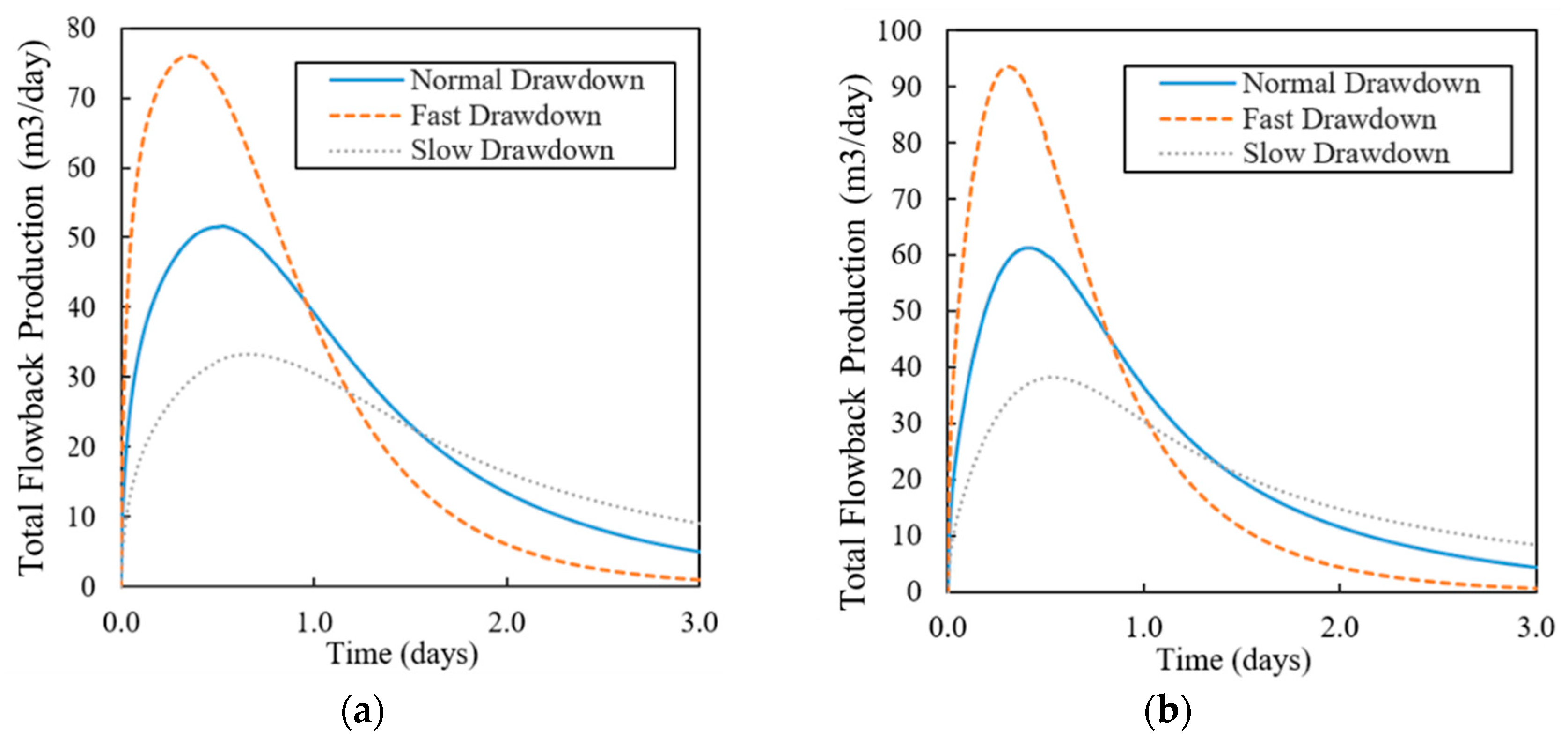
6.3. Flowback Responses with Different Drawdown Strategies
Botthomhole pressure is used as the inner boundary condition. Three different operational schemes are assumed in this study: 1) normal-pressure drawdown, 2) slow pressure drawdown, and 3. Fast pressure drawdown. The drawdown coefficient
a in Equation (68) is ranging from 20,0000, 10,0000, to 50,000 to represent slow, normal and fast drawdown cases, respectively. Simulation results for the two fracture networks are shown in
Figure 14. The influence of botthomhole pressure drawdown on flowback is similar in the two fracture networks. The initial flowback rate is high, but it also declines faster when the bottomhole pressure drawdown is implemented more aggressively. A faster pressure drawdown results in a higher cleanup rate. However, even though an initial aggressive flowback rate may accelerate the onset of hydrocarbon production, excessively high initial flowback rates may cause proppant flowback and damage to the fracture conductivity as a result of large drag forces driven by the high pressure-gradient forming along the fracture. It can be seen in
Figure 14 that using the normal drawdown scheme, we can still achieve a good fracking fluid recovery in the late flowback period in comparison to the aggressive drawdown case, however, a concrete conclusion requires coupling with oil flow from the matrix.
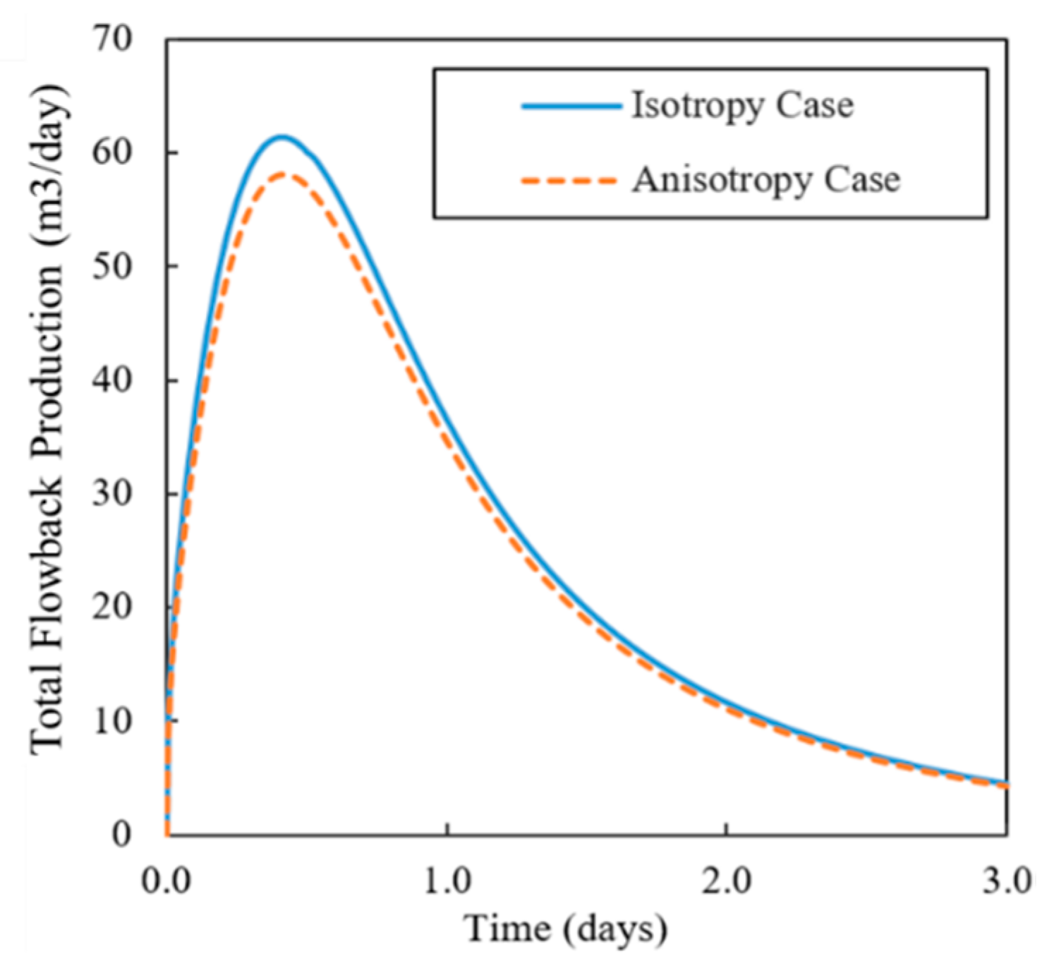
6.4. Flowback Responses with Isotropic Fracture and Anisotropic Fracture Sets
In general, it is expected that the fracture’s width decreases with distance from the wellbore. In orthogonal fracture network, while the difference between maximum horizontal stress (
) and minimum horizontal stress (
) is not significant, fractures’ width is expected to remain almost the same in different directions. However, when
is considerably larger than
, it is reasonable to expect that opening for fractures perpendicular to the maximum horizontal stress to be smaller than the one for fractures perpendicular to the minimum horizontal stress. Thus, it makes sense to examine the effect of the difference between maximum and minimum horizontal stresses on the flowback behavior in orthogonal fracture networks (like
Figure 5b). The total fracture volume is the same as the volume in the base case, however, the fractures’ width is assumed to be different depending on the fracture direction. We assumed that the fracture width in one direction to be 10% higher than the isotropic case while the fracture width in the other direction is 10% lower than the isotropic case. We observe that tectonic stress anisotropy would decrease the flowrate slightly as shown in
Figure 15, which is due to the fact that increasing anisotropy can reduce the overall connectivity. However, a concrete conclusion required coupled geomechanical analyses. The difference between the flowrate in the two cases gradually increases till reaching the peak rates and then starts to decrease. The peak of flowback rate decreased about 10% and average flowback rate decreased about 5% in comparison to the case in which the difference between
and
is not significant. This indicates that the water recovery is slightly higher in the formation which has a smaller difference between
and
6.5. Flowback Responses with Constant Compressibility and Variable Compressibility Models
In current works, flowback analysis is based on the assumption that fracture compressibility remains constant during flowback and production, which indeed according to Equation (60) should be a function of the fracture width and the effective proppant stress. Here, we examine the error that may arise from this assumption.
Figure 16 shows that in both fracture networks, the flowback by assuming constant fracture compressibility leads to underestimating flowrate peak and overestimating later production. The result suggests that the flowback analysis using constant compressibility can overestimate the fracture compressibility at the end of the flowback production. By using the proposed semi-analytical model, we can model flowback rate more accurately by dropping the invalid assumption of constant compressibility that can benefit subsequent inverse analyses.
In addition, all the above case studies indicate that with the same fracture volume, an orthogonal fracture network will provide higher flowback production at an early time while the depletion is faster as well. This is because fracture connectivity is higher in orthogonal fracture network.
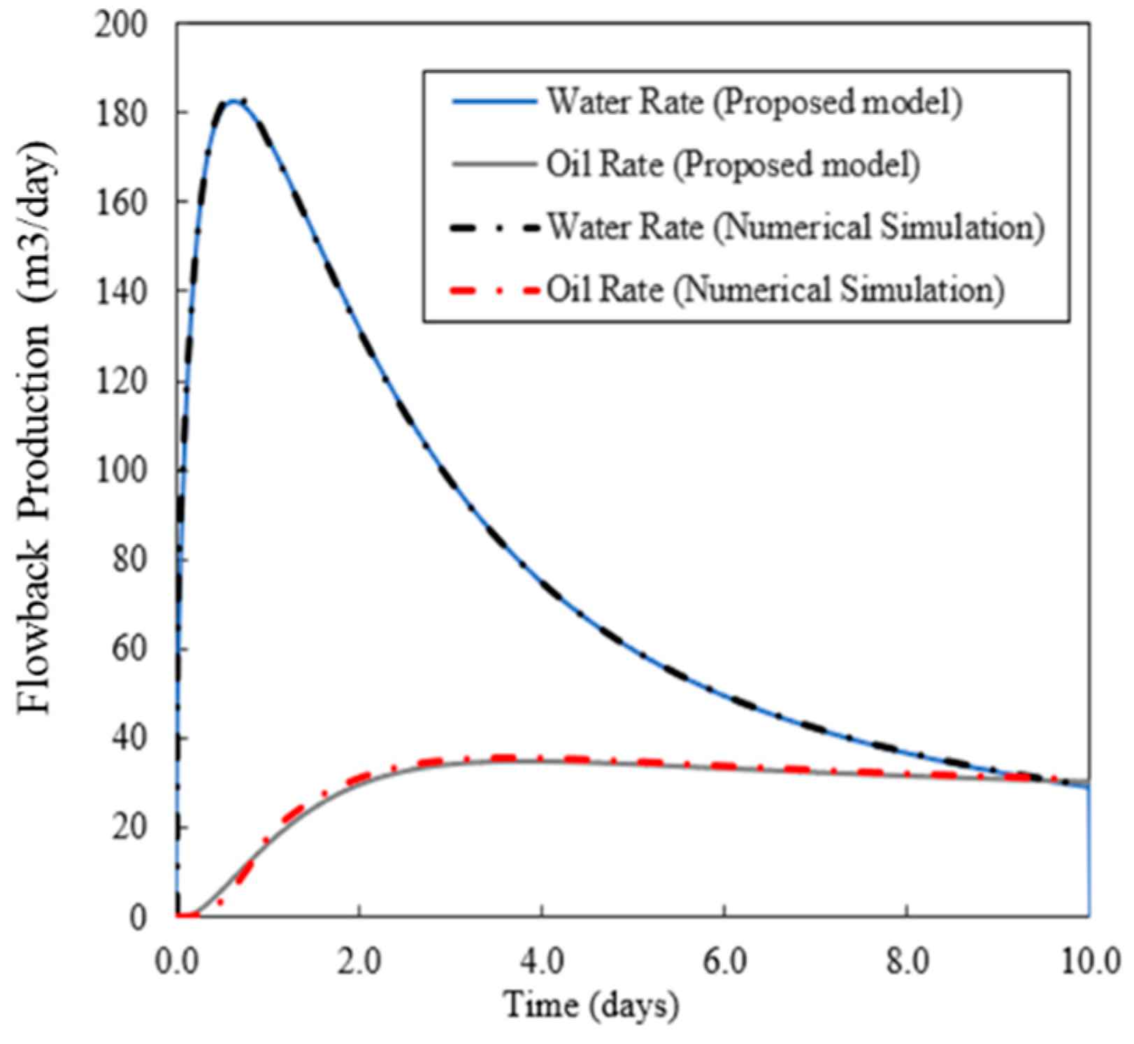
6.6. Applicability/Limitation of the Proposed Closed-Chamber Solution
The proposed semi-analytical solution presented in this paper only considers fluid flow inside the fracture network. Basically, the matrix flow is neglected in this solution as it takes a while for the reservoir fluid to enter the fracture. In order to gain an insight into the limitation of the proposed closed-chamber solution, we derived a two-phase flowback solution with a matrix influx for bi-wing fractures. The proposed solution with matrix inflow has been validated by CMG as shown in
Figure 17 with the input data listed in
Table 3. To test the accuracy of the proposed model in the extreme case when oil flux is significant, the oil saturation of the matrix is set to be one. Drawdown coefficient is 50,000 to represent an aggressive choke strategy. To capture the worst-case scenario to limit our flowback solution, the reservoir breakthrough pressure is set to be equal to the initial fracture pressure in the model with a formation influx. However, the true reservoir pressure is much lower than the fracture pressure at the beginning of flowback, additionally, there would be a huge capillary effect which blocks the formation fluid from entering the fracture. Therefore, lower breakthrough pressure should be used in practical analyses. The result indicates that the two-phase flowback solution with matrix oil influx is accurate while its computational cost is much lower than numerical simulation. However, it is worth noting that the model has more error when the oil velocity in matrix is high. This error is rooted in the definition of our two-phase pseudo-pressure, in which the saturation gradient inside the fracture cannot be captured accurately as a continuous function in the case of the large pressure gradient. However, this situation rarely happens during flowback in shale oil reservoirs due to the extremely low permeability of the matrix. This solution is only developed for simple fracture geometries and despite the first solution, this solution cannot be applied to complex fracture networks. But this solution can still serve as a tool to gain insight on the time limitation of the semi-analytical model, i.e., determine when matrix inflow starts to dominate the flowback flow.
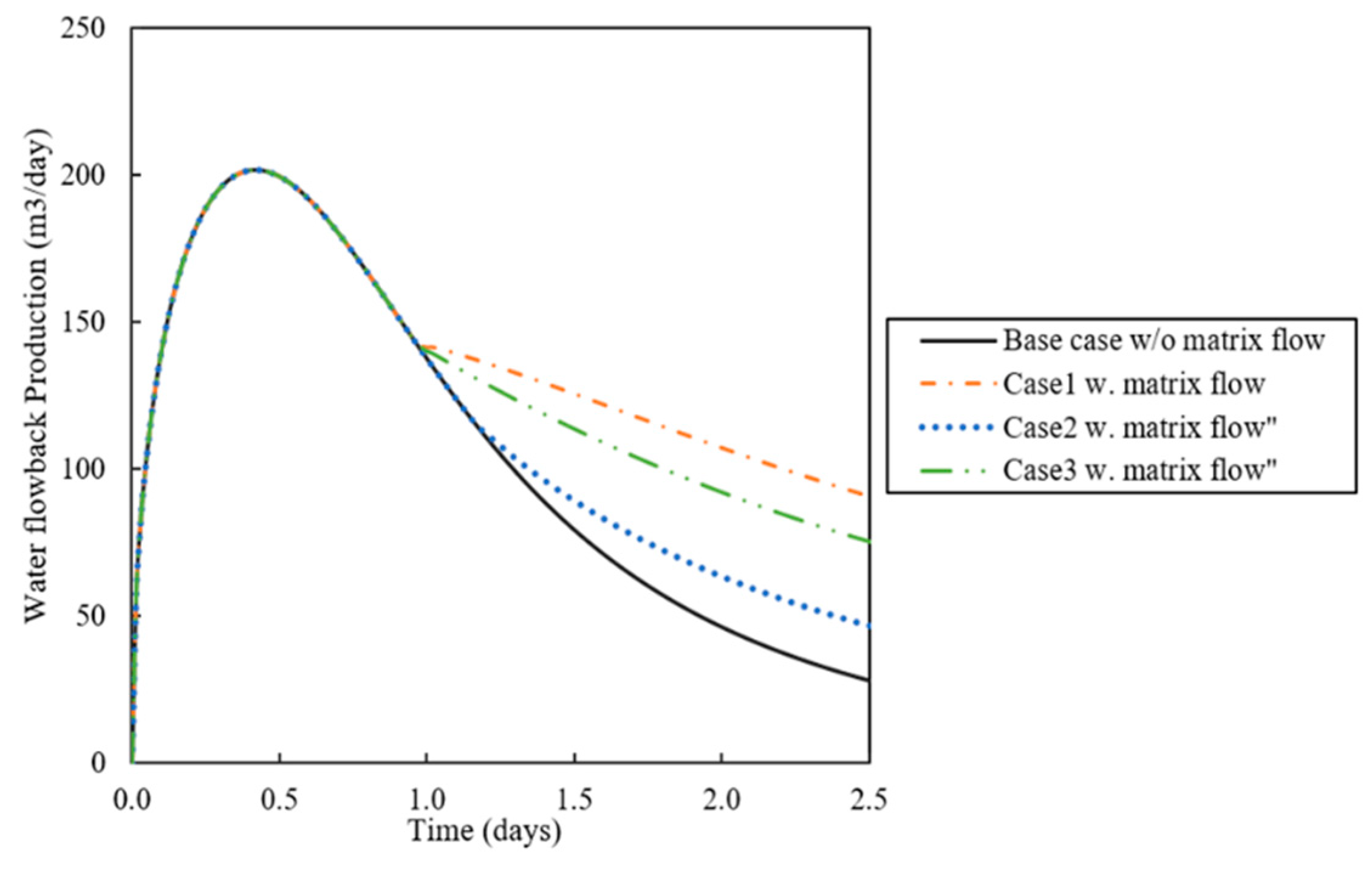
We did three case studies to examine the allowable time interval to use the proposed close-chamber solution. All other inputs are similar to the validation case shown in
Table 3. The criteria that we used to define transition time from the fracture linear flow to the matrix linear flow is the time that the flowback rate from the proposed solution deviates more than 20% from the flowback calculated from the solution with matrix oil influx, the model is considered inapplicable hereafter.
Figure 18 shows the comparison of the flowrates with and without matrix flow. The results show that the time when the proposed solution without oil matrix influx becomes invalid is 25, 27, and 35 hours for ases 1 to 3, respectively. Case 1 has the highest oil production among all the cases which makes the applicable time relatively short in comparison to the other two cases. Breakthrough pressure is 2.3 × 10
7 Pa. In case 2, we consider the formation has a smaller pore diameter (i.e., less porosity, less permeability, and higher capillary pressure). Porosity and permeability used is 0.03 and 1 × 10
−19 , respectively. The breakthrough pressure is decreased to 1.9 × 10
7 Pa. The significant capillary effect postpones the oil breakthrough time. The result indicates the model can be applied for an extended time in shale reservoirs with extremely small pore sizes. In case 3, we consider the formation of oil is more viscous, so oil viscosity is increased to 0.002 Pa·s. When the reservoir fluid is more viscous, matrix oil influx will be slower and the flowback model can be used for a longer time. From the applicability analysis, we show that the proposed semi-analytical solution is working for at least one day or longer times depending to reservoir properties. The allowable time window for this analysis is long enough to make data collection feasible. However, we suggest increasing data collection frequency for more accurate inverse analysis.
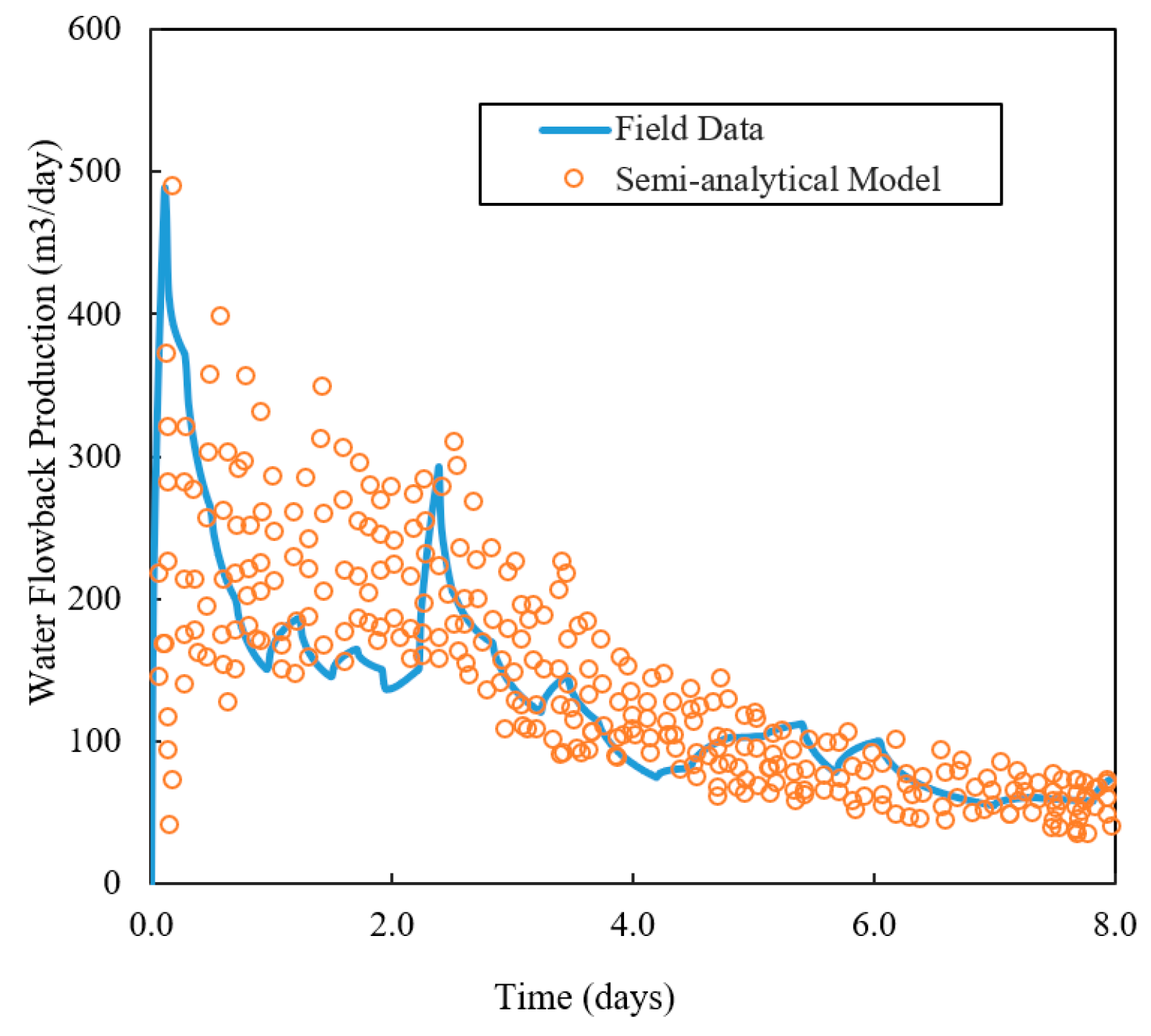
6.7. Field Example
To test the practical applicability of the proposed model, we use the flowback data from a multi-fractured horizontal well completed in a tight oil reservoir in Western Canada [
5]. First, using the proposed solution for planar fractures with matrix influx, we showed that a similar production match can be achieved as shown in
Figure 19. As we did not include resolved gas in oil in our model, the history matching is based on water production data only.
As indicated in their study, the authors pointed out that a larger than typical value of fracture width is used in the history matching to account tor activated secondary fractures during stimulation.


