Electricity Consumption Prediction of Solid Electric Thermal Storage with a Cyber–Physical Approach

 ,
,  ,
,
Abstract
1. Introduction
- To the best of the authors’ knowledge, this is the first work to use the cyber–physical approach to predict the SETS’ load change. The physical and cyber components of SETS are integrated.
- Using the existing knowledge of thermodynamics, a SETS PM is developed by considering the customers’ behavior characteristics.
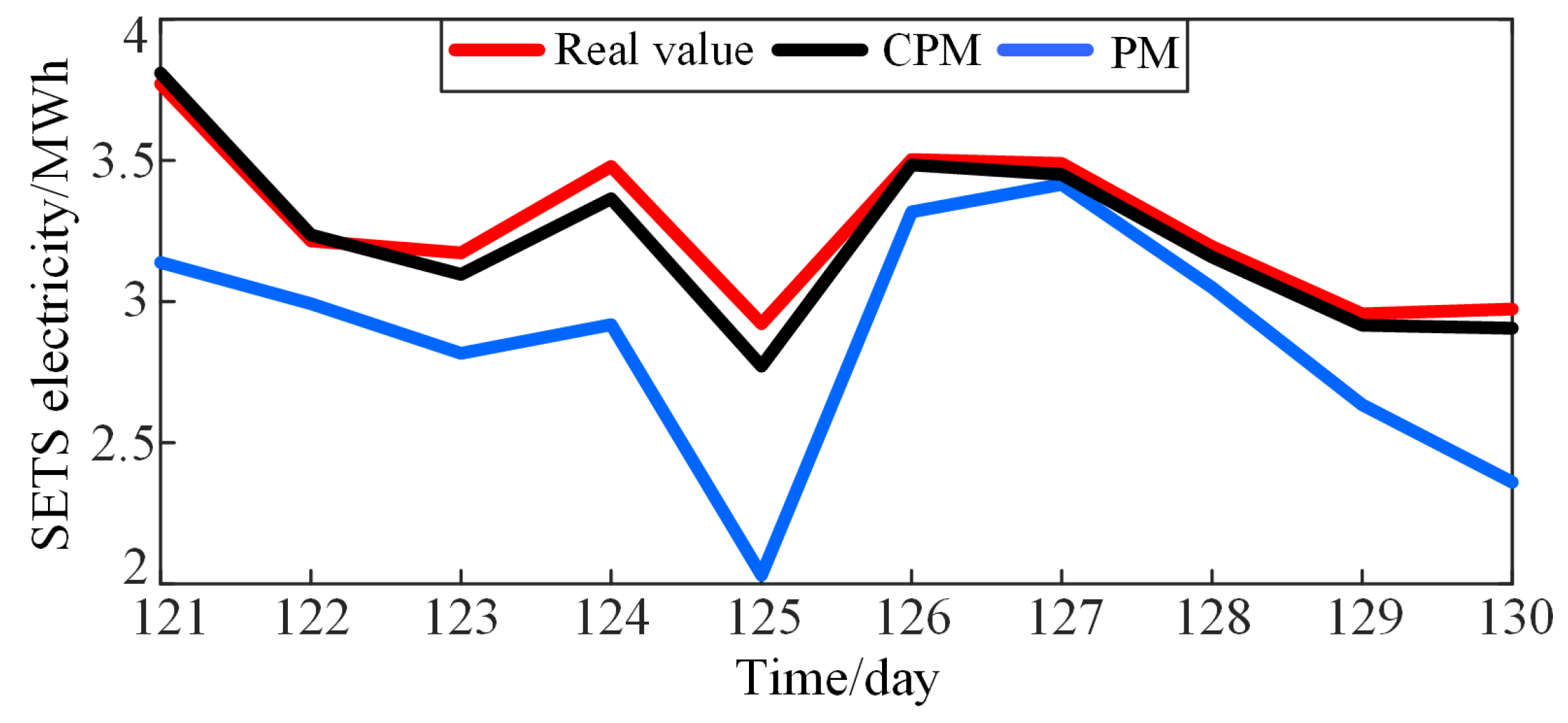
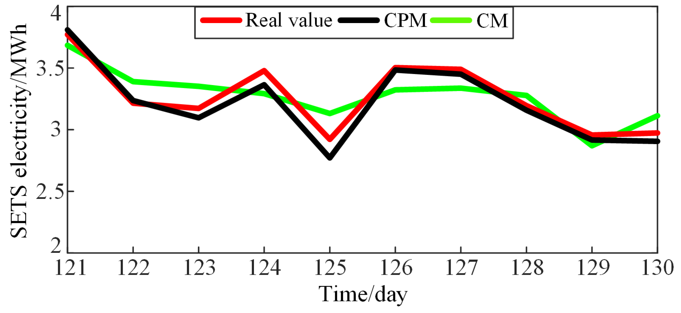
- The load data of 1MW SETS is used to validate the CPM, and the results show that, compared with the PM and the CM, the maximum relative errors (MRE) with the CPM are reduced to 25.4% and 4.8%, respectively.
2. PM of SETS
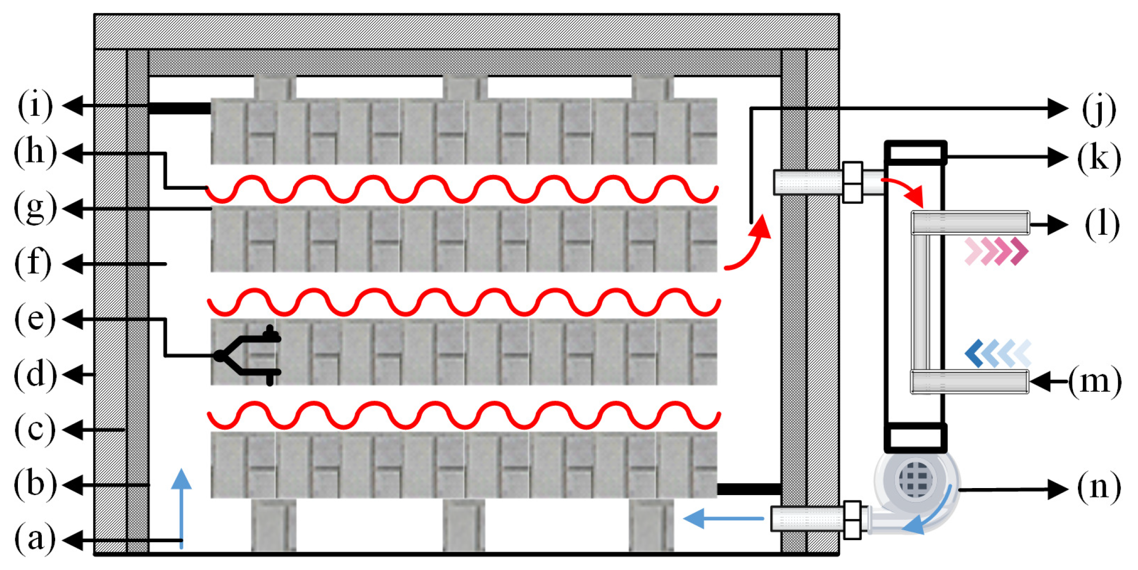
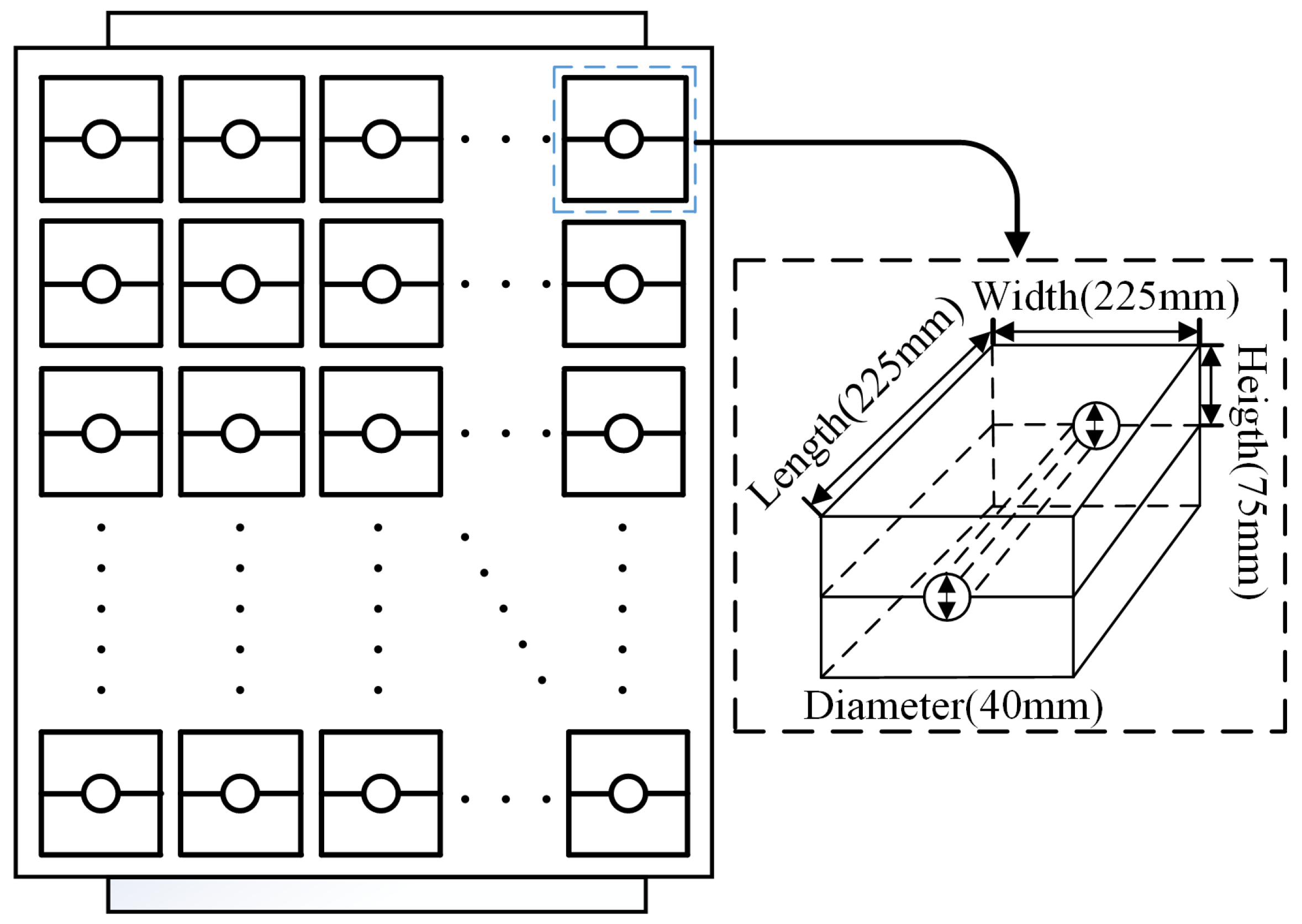
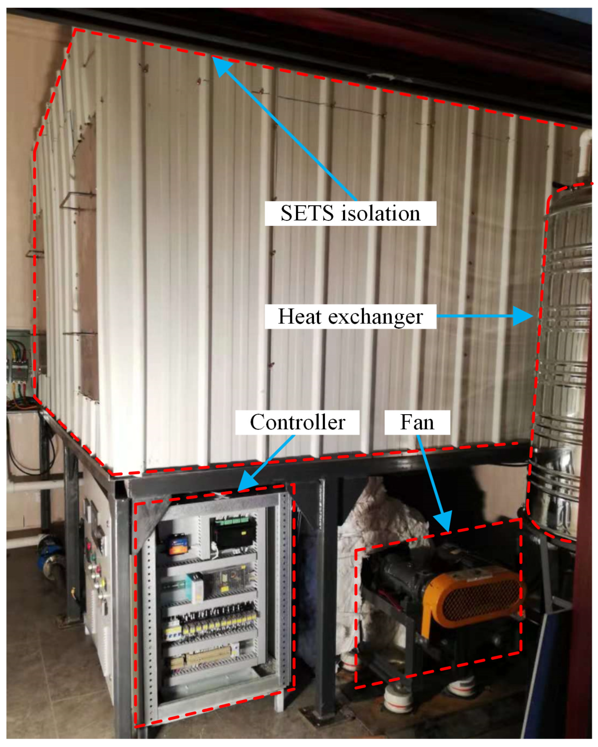
2.1. SETS Structure
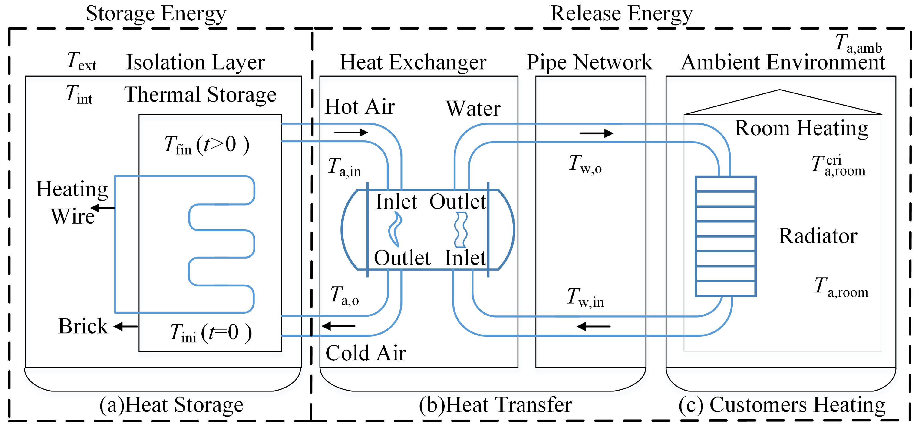
2.2. Principle
2.3. Thermal Energy Storage
2.3.1. Thermal Convection
2.3.2. Thermal Radiation
2.3.3. Thermal Conduction
2.4. Thermal Bricks Energy Release
2.4.1. Heat Transfer
2.4.2. Customers Heating
2.5. Customers’ Behavior Characteristics Extraction
| Algorithm 1 The behavior characteristics extraction algorithm process. |
|
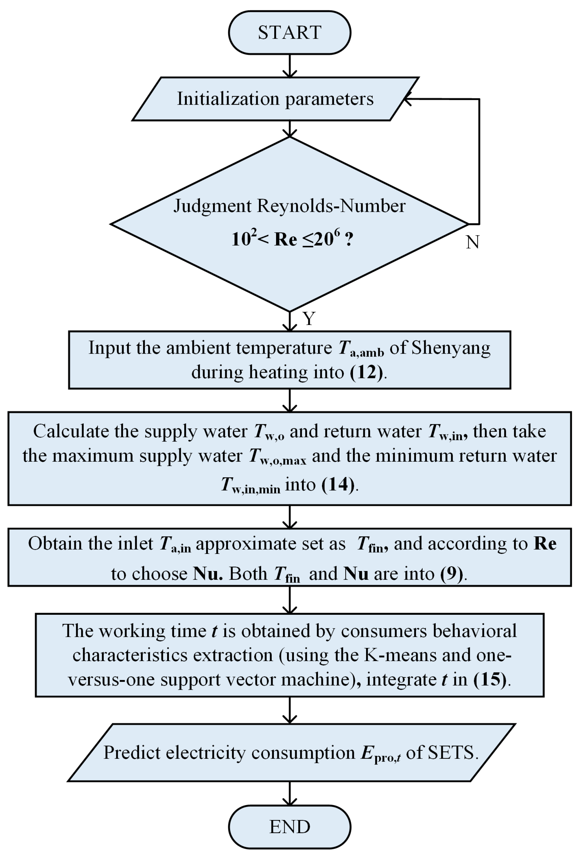
2.6. Summary of the PM Prediction
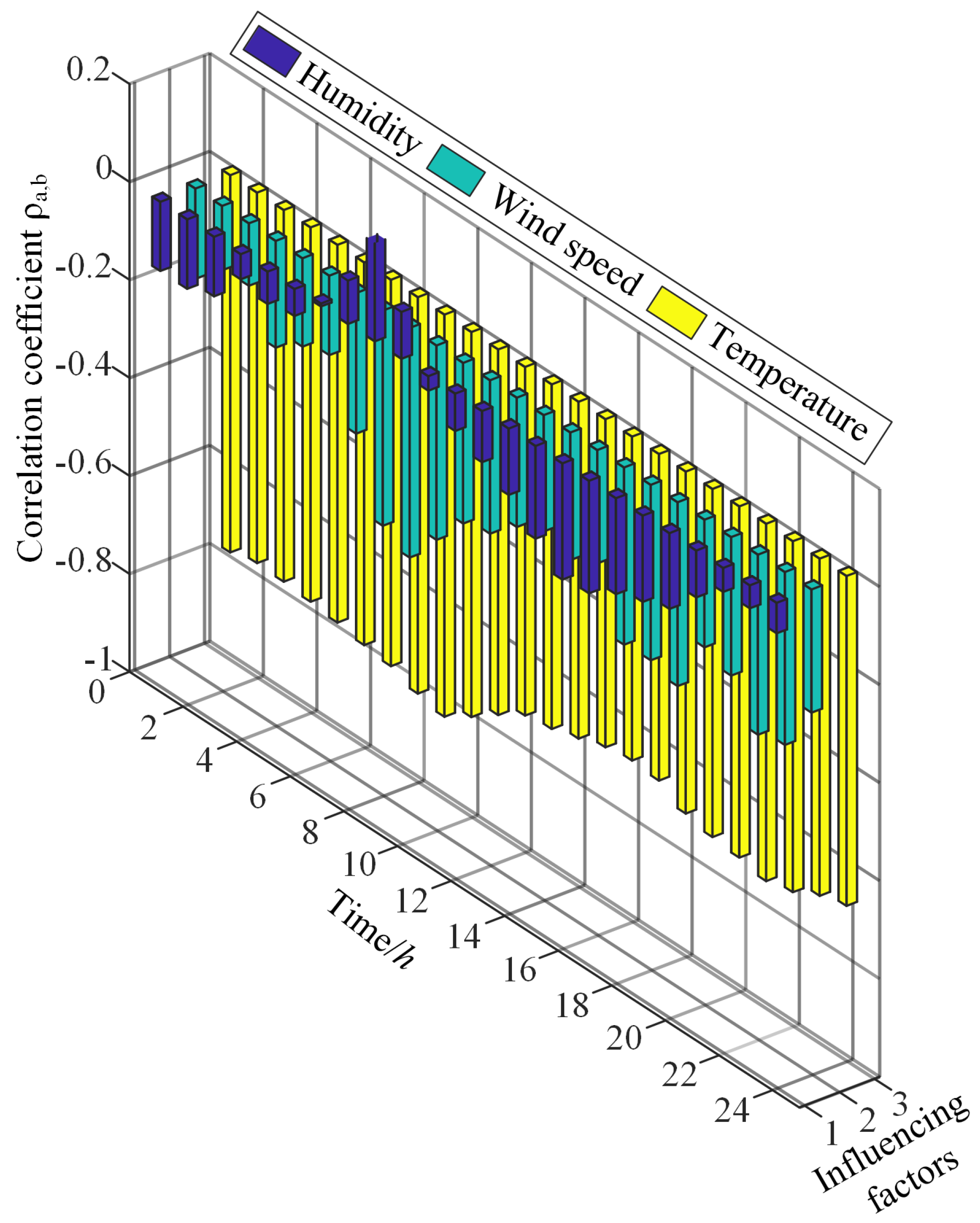
2.7. Influencing Factors
3. Cyber–Physical Approach
4. Validation
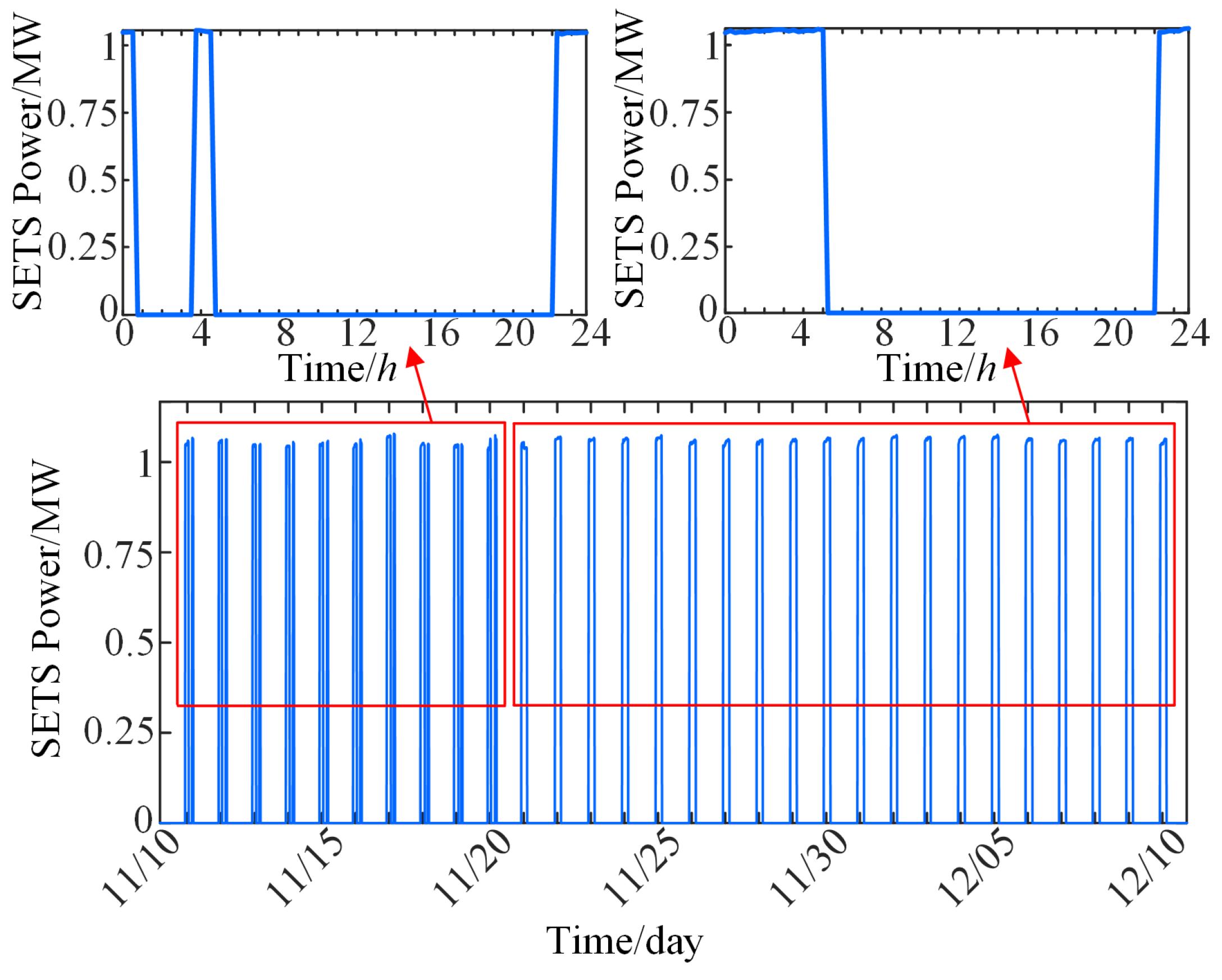
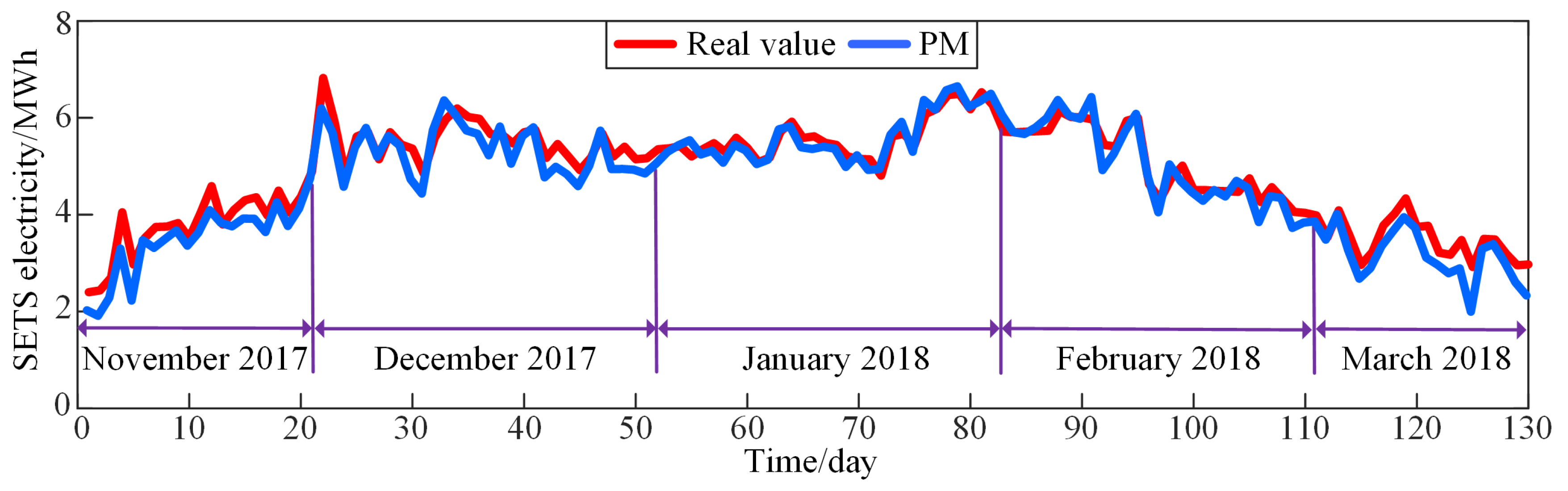
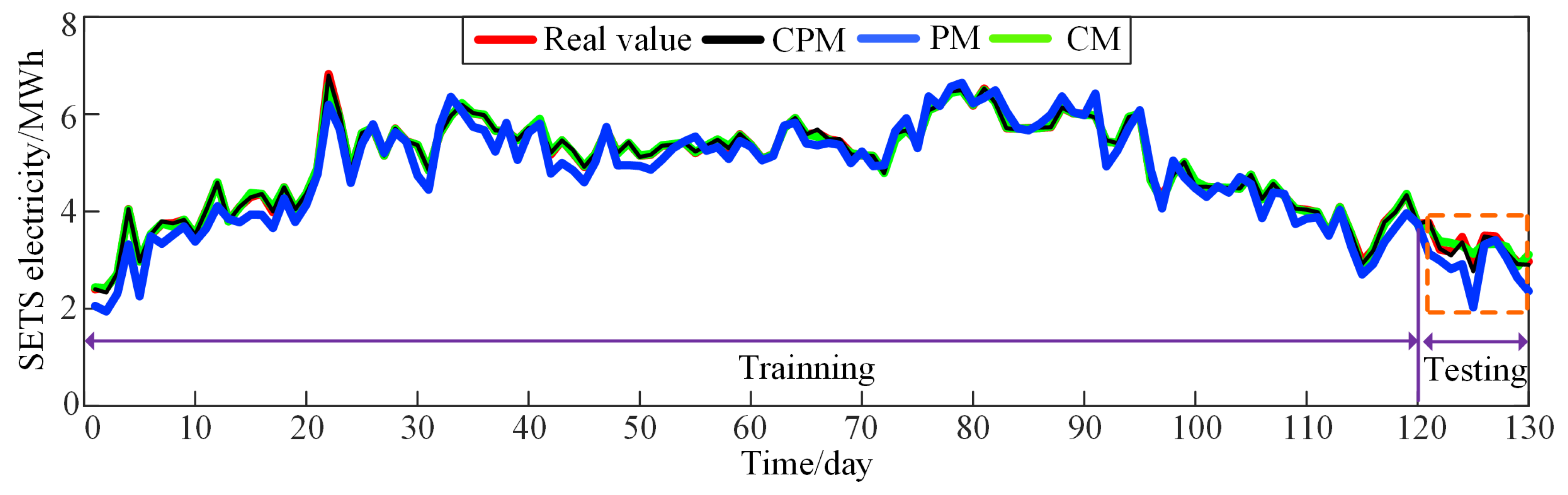
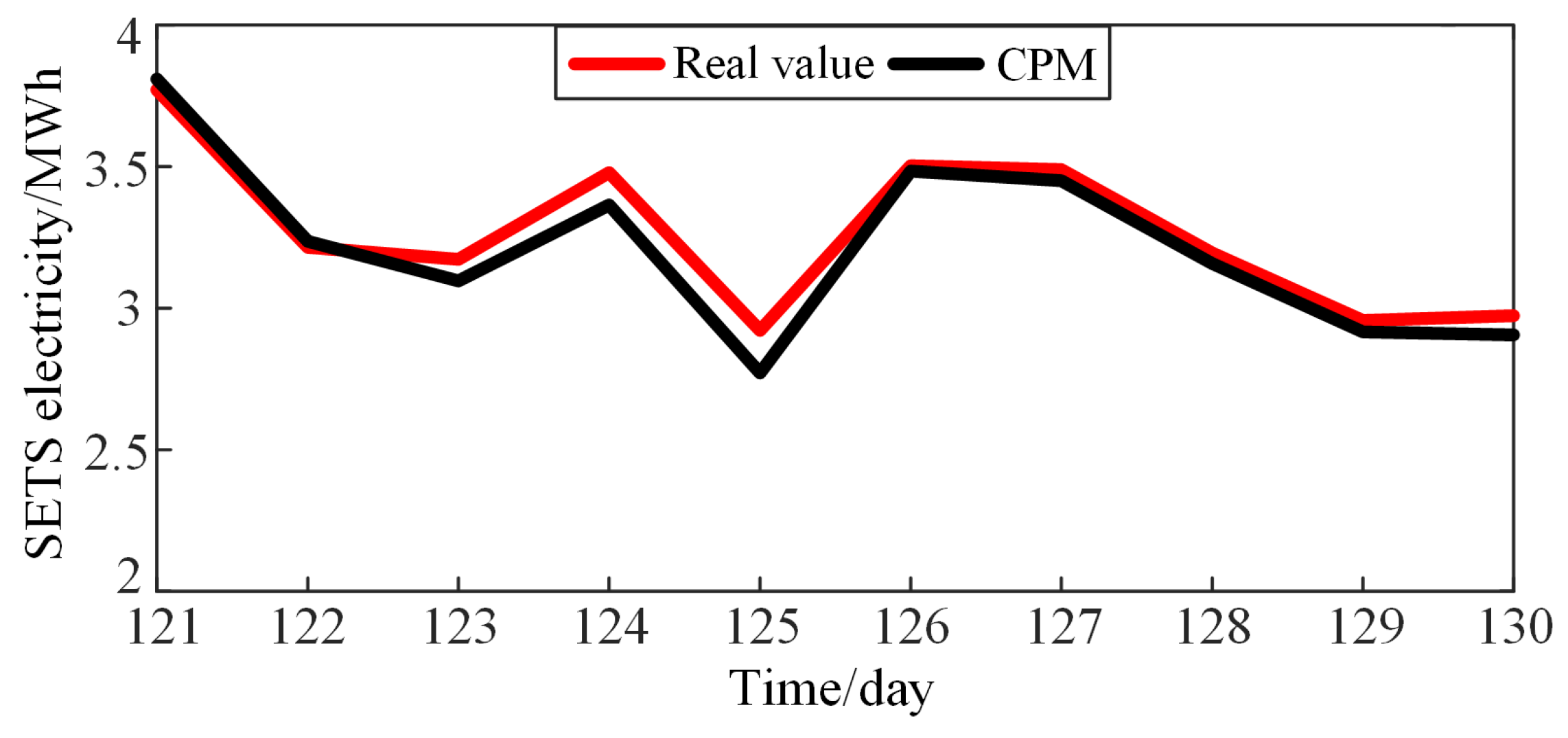
4.1. Comparison of CPM with Real Value
4.2. Comparison of CPM with PM
4.3. Comparison of CPM with CM
5. Conclusions
- Thermal storage is an effective method for peak shaving and dispatching in power system. The electricity consumption prediction of SETS is worth to explore the combination with the heat and power generation unit.
- The application of the proposed cyber–physical model in other resources of the power system is recommended to be studied.
Author Contributions
Funding
Conflicts of Interest
References
- Ibrahim, D. On thermal energy storage systems and applications in buildings. Energy Build. 2002, 34, 377–388. [Google Scholar]
- Cisek, P.; Taler, D. Numerical and experimental study of a solid matrix electric thermal storage unit dedicated to environmentally friendly residential heating system. Energy Build. 2016, 130, 747–760. [Google Scholar] [CrossRef]
- Sauter, P.S.; Solanki, B.V.; Cañizares, C.A.; Bhattacharya, K.; Hohmann, S. Electric thermal storage system impact on northern communities’ microgrids. IEEE Trans. Smart Grid 2019, 10, 852–863. [Google Scholar] [CrossRef]
- Wong, S.; Pinard, J.P. Opportunities for smart electric thermal storage on electric grids with renewable energy. IEEE Trans. Smart Grid. 2017, 8, 1014–1022. [Google Scholar] [CrossRef]
- Cooke, W.B.H.; Hardy, R.H.S.; Sulatisky, M.T. Thermal energy storage in forced-air electric furnaces. IEEE Trans. Ind. Appl. 1980, IA-16, 127–133. [Google Scholar] [CrossRef]
- Bedouani, B.Y.; Moreau, A.; Parent, M.; Labrecque, B. Central electric thermal storage (ETS) feasibility for residential applications: part 1. numerical and experimental study. Int. J. Energy Res. 2001, 25, 53–72. [Google Scholar] [CrossRef]
- Wang, X.; Zhang, M.; Ren, F. Learning customer behaviors for effective load forecasting. IEEE Trans. Knowl. Data Eng. 2019, 31, 938–951. [Google Scholar] [CrossRef]
- Quilumba, F.L.; Lee, W.J.; Huang, H.; Wang, D.Y.; Szabados, R.L. Using smart meter data to improve the accuracy of intraday load forecasting considering customer behavior similarities. IEEE Trans. Smart Grid 2015, 6, 911–918. [Google Scholar] [CrossRef]
- Xu, G.; Hu, X.; Liao, Z.; Xu, C.; Yang, C.; Deng, Z. Experimental and numerical study of an electrical thermal storage device for space heating. Energies 2018, 11, 2180. [Google Scholar] [CrossRef]
- Taylor, J.W. Short-term load forecasting with exponentially weighted methods. IEEE Trans. Power Syst. 2012, 27, 458–464. [Google Scholar] [CrossRef]
- Wu, L.; Shahidehpour, M. A hybrid model for integrated day-ahead electricity price and load forecasting in smart grid. IET Gener. Transm. Distrib. 2014, 8, 1937–1950. [Google Scholar] [CrossRef]
- Rejc, M.; Pantoš, M. Short-term transmission-loss forecast for the Slovenian transmission power system based on a fuzzy-logic decision approach. IEEE Trans. Power Syst. 2011, 26, 1511–1521. [Google Scholar] [CrossRef]
- Jiang, H.; Zhang, Y.; Muljadi, E.; Zhang, J.J.; Gao, D.W. A short-term and high-resolution distribution system load forecasting approach using support vector regression with hybrid parameters optimization. IEEE Trans. Smart Grid 2018, 9, 3341–3350. [Google Scholar] [CrossRef]
- Rafiei, M.; Niknam, T.; Aghaei, J.; Shafie-Khah, M.; Catalão, J.P.S. Probabilistic load forecasting using an improved wavelet neural network trained by generalized extreme learning machine. IEEE Trans. Smart Grid 2018, 9, 6961–6971. [Google Scholar] [CrossRef]
- Hong, T.; Wilson, J.; Xie, J. Long term probabilistic load forecasting and normalization with hourly information. IEEE Trans. Smart Grid 2014, 5, 456–462. [Google Scholar] [CrossRef]
- Thouvenot, V.; Pichavant, A.; Goude, Y.; Antoniadis, A.; Poggi, J.M. Electricity forecasting using multi-stage estimators of nonlinear additive models. IEEE Trans. Power Syst. 2016, 31, 3665–3673. [Google Scholar] [CrossRef]
- Idowu, S.; Saguna, S.; Åhlund, C.; Schelén, O. Applied machine learning: Forecasting heat load in district heating system. Energy Build. 2016, 133, 478–488. [Google Scholar] [CrossRef]
- Wang, Z.; Wang, J.; Zhao, L.; Jia, S. A thermal energy usage prediction method for electric thermal storage heaters based on deep learning. In Proceedings of the 2019 IEEE 4th International Conference on Cloud Computing and Big Data Analysis, Chengdu, China, 12–15 April 2019. [Google Scholar]
- Nigitz, T.; Gölles, M. A generally applicable, simple and adaptive forecasting method for the short-term heat load of consumers. Appl. Energy 2019, 241, 73–81. [Google Scholar] [CrossRef]
- Macana, C.A.; Quijano, N.; Mojica-Nava, E. A survey on cyber physical energy systems and their applications on smart grids. In Proceedings of the 2011 IEEE PES Conference on Innovative Smart Grid Technologies Latin America, Medellin, Colombia, 19–21 October 2011. [Google Scholar]
- Seshia, S.A.; Hu, S.; Li, W.; Zhu, Q. Design automation of cyber–physical systems: Challenges, advances, and opportunities. IEEE Trans. Comput-Aided Des. Integr. Circuits Syst. 2017, 36, 1421–1434. [Google Scholar] [CrossRef]
- Dai, Y.; Chen, L.; Min, Y.; Chen, Q.; Hao, J.; Hu, K. Modeling and analysis of electrical heating system based on entransy dissipation-based thermal resistance theory. In Proceedings of the 2016 IEEE Power and Energy Society General Meeting, Boston, MA, USA, 17–21 July 2016. [Google Scholar]
- Alawadhi, E.M. Thermal analysis of a building brick containing phase change material. Energy Build. 2008, 40, 351–357. [Google Scholar] [CrossRef]
- Gao, W.; Zhao, J.; Li, X.; Zhao, H.; Zhang, Y.; Wu, X. Heat transfer characteristics of carbon dioxide cross flow over tube bundles at supercritical pressures. Appl. Therm. Eng. 2019, 158, 1–16. [Google Scholar] [CrossRef]
- Attonaty, K.; Stouffs, P.; Pouvreau, J.; Oriol, J.; Deydier, A. Thermodynamic analysis of a 200 MWh electricity storage system based on high temperature thermal energy storage. Energy 2019, 172, 1132–1143. [Google Scholar] [CrossRef]
- Liu, L.; Huang, H.; Hu, S. Lorenz chaotic system-based carbon nanotube physical unclonable functions. IEEE Trans. Comput-Aided Des. Integr. Circuits Syst. 2018, 37, 1408–1421. [Google Scholar] [CrossRef]
- Hashemi, S.; Yang, Y.; Mirzamomen, Z.; Kangavari, M. Adapted one-versus-all decision trees for data stream classification. IEEE Trans. Knowl. Data Eng. 2009, 21, 624–637. [Google Scholar] [CrossRef]
- Li, Y.; Wang, Y.; Hu, S. Online generative adversary network based measurement recovery in false data injection attacks: a cyber–physical approach. IEEE Trans. Ind. Inform. 2019. [Google Scholar] [CrossRef]
- Liu, Y.; Zhou, Y.; Hu, S. Combating coordinated pricing cyberattack and energy theft in smart home cyber–physical systems. IEEE Trans. Comput-Aided Des. Integr. Circuits Syst. 2018, 37, 573–586. [Google Scholar] [CrossRef]
- Zhou, Y.; Liu, Y.; Hu, S. Energy theft detection in multi-tenant data centers with digital protective relay deployment. IEEE Trans. Sustain. Comput. 2018, 3, 16–29. [Google Scholar] [CrossRef]
- Chen, X.; Zhang, D.; Wang, L.; Jia, N.; Kang, Z.; Zhang, Y.; Hu, S. Design automation for interwell connectivity estimation in petroleum cyber–physical systems. IEEE Trans. Comput-Aided Des. Integr. Circuits Syst. 2017, 36, 255–264. [Google Scholar] [CrossRef]


| Month | 2017.11 | 2017.12 | 2018.1 | 2018.2 | 2018.3 |
|---|---|---|---|---|---|
| Date | 10–30 | 1–31 | 1–31 | 1–28 | 1–19 |
| RMSE | 372.05 | 310.29 | 167.36 | 227.1 | 389.45 |
| MAE | 323.36 | 264.99 | 139.33 | 183.92 | 318.54 |
| MAPE% | 9.08 | 4.82 | 2.49 | 3.75 | 9.53 |
| Average | 3805 | 5526.9 | 5616 | 5035.1 | 3470.8 |
| Average | 3486.3 | 5323.3 | 5610 | 4990.2 | 3152.7 |
| Parts | Symbol | Number | Unit | Symbol | Number | Unit |
|---|---|---|---|---|---|---|
| Bricks | 150 | 105 | ||||
| 0.225 | 0.225 | |||||
| 0.075 | 0.02 | |||||
| L-row | 7 | W-row | 16 | |||
| H-row | 43 | 0.5 | ||||
| Exchanger | 45 | C | 65 | C | ||
| 1.093 | 4.174 | |||||
| 30,936 | 15 | |||||
| 1 | m | |||||
| Isolation | 0.5 | 0.101 | ||||
| 0.05 | 0.13 | |||||
| 50 | ||||||
| Room | 18 | −16.9 | ||||
| 0.0574 | 79.38 | |||||
| 0.706 | 0.687 | |||||
| 0.287 |
| Day | Real Value | CPM | MRE | PM | MRE | CM | MRE |
|---|---|---|---|---|---|---|---|
| 121 | 3.771 | 0.038 | 1 | 0.632 | 16.7 | 0.086 | 2.3 |
| 122 | 3.216 | 0.02 | 0.6 | 0.223 | 6.9 | 0.174 | 5.4 |
| 123 | 3.173 | 0.076 | 2.4 | 0.356 | 11.2 | 0.179 | 5.6 |
| 124 | 3.479 | 0.113 | 3.3 | 0.56 | 16.1 | 0.186 | 5.3 |
| 125 | 2.922 | 0.15 | 5 | 0.891 | 30.4 | 0.21 | 7.2 |
| 126 | 3.503 | 0.018 | 0.5 | 0.185 | 5.2 | 0.179 | 5.1 |
| 127 | 3.489 | 0.039 | 1.1 | 0.074 | 2.1 | 0.152 | 4.4 |
| 128 | 3.195 | 0.037 | 1.1 | 0.145 | 4.5 | 0.083 | 2.6 |
| 129 | 2.956 | 0.039 | 1.3 | 0.321 | 10.8 | 0.086 | 2.9 |
| 130 | 2.973 | 0.067 | 2.3 | 0.613 | 20.6 | 0.14 | 4.7 |
© 2019 by the authors. Licensee MDPI, Basel, Switzerland. This article is an open access article distributed under the terms and conditions of the Creative Commons Attribution (CC BY) license (http://creativecommons.org/licenses/by/4.0/).
Share and Cite
Ji, H.; Yang, J.; Wang, H.; Tian, K.; Okoye, M.O.; Feng, J. Electricity Consumption Prediction of Solid Electric Thermal Storage with a Cyber–Physical Approach. Energies 2019, 12, 4744. https://doi.org/10.3390/en12244744
Ji H, Yang J, Wang H, Tian K, Okoye MO, Feng J. Electricity Consumption Prediction of Solid Electric Thermal Storage with a Cyber–Physical Approach. Energies. 2019; 12(24):4744. https://doi.org/10.3390/en12244744
Chicago/Turabian StyleJi, Huichao, Junyou Yang, Haixin Wang, Kun Tian, Martin Onyeka Okoye, and Jiawei Feng. 2019. "Electricity Consumption Prediction of Solid Electric Thermal Storage with a Cyber–Physical Approach" Energies 12, no. 24: 4744. https://doi.org/10.3390/en12244744
APA StyleJi, H., Yang, J., Wang, H., Tian, K., Okoye, M. O., & Feng, J. (2019). Electricity Consumption Prediction of Solid Electric Thermal Storage with a Cyber–Physical Approach. Energies, 12(24), 4744. https://doi.org/10.3390/en12244744