Article

Partial Discharge Pattern Recognition of Gas-Insulated Switchgear via a Light-Scale Convolutional Neural Network

1
State Key Laboratory of Electrical Insulation and Power Equipment, Xi’an Jiaotong University, Xi’an 710049, China
2
School of Computer Science, Xi’an Jiaotong University, Xi’an 710049, China
*
Author to whom correspondence should be addressed.
Energies 2019, 12(24), 4674; https://doi.org/10.3390/en12244674
Submission received: 9 November 2019 / Revised: 3 December 2019 / Accepted: 5 December 2019 / Published: 9 December 2019

Abstract

:
Partial discharge (PD) is one of the major form expressions of gas-insulated switchgear (GIS) insulation defects. Because PD will accelerate equipment aging, online monitoring and fault diagnosis plays a significant role in ensuring safe and reliable operation of the power system. Owing to feature engineering or vanishing gradients, however, existing pattern recognition methods for GIS PD are complex and inefficient. To improve recognition accuracy, a novel GIS PD pattern recognition method based on a light-scale convolutional neural network (LCNN) without artificial feature engineering is proposed. Firstly, GIS PD data are obtained through experiments and finite-difference time-domain simulations. Secondly, data enhancement is reinforced by a conditional variation auto-encoder. Thirdly, the LCNN structure is applied for GIS PD pattern recognition while the deconvolution neural network is used for model visualization. The recognition accuracy of the LCNN was 98.13%. Compared with traditional machine learning and other deep convolutional neural networks, the proposed method can effectively improve recognition accuracy and shorten calculation time, thus making it much more suitable for the ubiquitous-power Internet of Things and big data.

1. Introduction

Gas-insulated switchgear (GIS) is widely used in power systems because of its small footprint, high reliability, low environmental impact, and maintenance-free features. Potential risks exist, however, in design, manufacturing, transportation, installation, and operation and maintenance, which may further give rise to latent GIS failures [1,2,3]. Because the GIS is one of the main control and protection components of the power system, once it fails, it will significantly shock the power grid, not only causing large-scale power outages and negatively affecting power supply reliability but also resulting in massive economic losses. Therefore, effective detection of GIS latent defects and taking necessary measures before failures are of great importance in ensuring safe and reliable operation of the power grid while reducing maintenance time and cost.
The advancement of the construction of the ubiquitous-power Internet of Things (IoT) provides new opportunities for GIS fault diagnosis and challenges [4,5]. Exploring not only real-time rapid processing of GIS fault signals but also the ability to accurately identify fault diagnosis methods for GIS faults has become an urgent problem to be solved. According to the statistics, insulation faults are the main cause of accidents in GIS [6], and most insulation faults are manifested in the form of partial discharges (PDs), which will further accelerate equipment aging. Currently, the detection of insulation faults is mainly done by means of measuring sound, light-scale, heat, and electromagnetic waves and the decomposition of chemical products induced by PD [7]. Detection methods include pulse current, ultra-high-frequency (UHF), ultrasonic, optical detection, and gas decomposition product detection methods [8,9,10,11,12]. Among these methods, the UHF method is widely adopted because of its strong anti-interference ability and high detection sensitivity [13]. As a result of visible feature differences of different PD sources, these characteristics can be used for PD pattern recognition and classification.
Given the randomness of PD, traditional machine learning methods are widely applied to PD pattern recognition and classification. The current main classification methods are support vector machine, decision tree, random forest, neural network, and improved algorithms of the aforementioned methods [14,15,16,17,18]. Compared with the classification methods, feature extraction plays a more important role in pattern recognition, as the quality of the feature directly affects the performance of the classification algorithm. Numerous feature extraction methods involving time-resolved partial discharge (TRPD) and phase-resolved partial discharge (PRPD) have emerged, mainly including Fourier transforms, wavelet transforms, Hilbert transforms, empirical mode decomposition, S-parameter transformation, fractal parameters, and polar coordinate transformation [19,20,21,22,23,24,25]. The identification method based on PRPD mode has strong anti-interference ability; however, the synchronous phase of the high voltage side is not necessarily obtained in the field measurement, and this analysis method is difficult to implement when there is external electromagnetic interference. Since TRPD mode needs to analyze the relationship between different insulation defects and discharge pulse waveform, it is a direct analysis method closer to the discharge mechanism. Its data acquisition system is simple and can distinguish noise signals, which can be extended to PD detection of direct current (DC) equipment. Therefore, the recognition method based on the TRPD pattern has high research value [26,27,28].
Traditional machine learning methods exhibit excellent performance in PD pattern recognition classification. Their feature extraction methods, however, excessively rely on expert experience while massive manual interventions will lead to artificial error. At the same time, the features extracted by different algorithms can neither be shared nor are transferable, so it is difficult to guarantee that they are still the best in other algorithms [29]. To effectively solve this problem, deep learning methods that rely on automatic feature extraction are introduced into GIS PD pattern recognition. At present, these deep learning models include LeNet5, AlexNet, one-dimensional convolution, and long short-term memory (LSTM) models [30,31,32,33,34].
In the aforementioned methods, however, the input requirement of LeNet5 is 28 × 28, and shrinking the original image to such a small size may result in incomplete information utilization as well as low recognition accuracy of the TRPD pattern. Deepening of the network causes a vanishing gradient, which prevents AlexNet from being trained and significantly prolongs the model training time. This problem may become exacerbated with deepening of the network. Therefore, deep convolutional neural networks (CNNs) may not work in TRPD-based GIS PD pattern recognition. To solve the problem of insufficient utilization of feature information in traditional methods as well as the low recognition accuracy resulting from the vanishing gradient, a new method using a light-scale convolutional neural network (LCNN) is proposed in this paper. The proposed method can, to a large extent, optimize the time performance of the model for better application to IoT conditions. It can improve the recognition accuracy of the model in characterizing TRPD-based GIS PD features while greatly shortening the model training and testing time. Therefore, it can rapidly process failures in real time. The main contributions of this paper are as follows:
(1) An LCNN model is proposed for GIS PD pattern recognition. By combining experimental data and simulation data, it maximizes the stochastic simulation of PD and reduces the model’s dependence on expert experience via automatic feature extraction and full utilization of feature information. Hence, it effectively increases the accuracy of pattern recognition.
(2) The conditional variation auto-encoder is used for data enhancement. Considering the standardization of TRPD waveform images, it is difficult to meet the requirements by data enhancement methods, such as image rotation and transformation. This paper uses a conditional variation auto-encoder to generate new data for data enhancement. Meanwhile, through dropout, normalization, and other methods, it effectively reduces the model training and testing time, making it more applicable to the ubiquitous-power IoT context.
(3) The model is visualized by a deconvolution neural network and TensorBoard, and the “black-box” problem of CNNs is solved.

2. Proposed Method

2.1. Data Enhancement with Conditional Variation Auto-Encoder

Based on the raw sample, data enhancement is aimed at learning the sample features and reconstructing the samples in the same feature distributions through constructing a deep network. It can greatly increase the number of samples [35,36,37,38], thus improving classification performance. The technique, which originates from game theory, entails making the generator and discriminator in the network gradually achieve dynamic equilibrium (Nash equilibrium), so that the model can better learn the approximate feature distribution from the input samples. Since the acquired PD signals are stored in a unified standard manner, the image scaling can only introduce noise interference and cannot achieve data enhancement. Considering the standardization of TRPD waveform images, data enhancement methods through image rotation and transformation can result in enhanced data becoming difficult to classify as special samples. In PD pattern recognition, because of the relatively small number of total data sets, in this paper, a conditional variation auto encoder (CVAE) is adopted as the data enhancement model to increase the number of training data and improve the generalization ability of the model.
The basic idea of the CVAE algorithm is that each entry point, x μ i , is replaced by a respective hidden variable, z . Therefore, the final output, x ˜ , can be generated by a certain probability distribution, P θ ( x | z ) , which is assumed to be Gaussian. The decoder function, f θ ( z ) , can generate the final parameters of the generated distribution and itself is constrained by a set of uniform parameters, θ . At the same time, the encoder function, g θ ( x ) , can generate a parameter for each probability distribution, q ϕ ( z | x ) , which is also restrained by the parameter, θ . In training and testing, a label factor is added to the network learning image distribution. The condition of the label factor is set as y, and, in this sense, the specified image can be generated according to the label value.
The variational derivation indicates that an approximate distribution, p ( z ) , is needed in place of the distribution, q ϕ ( z | x ) . The similarity of the two distributions is usually measured by a function called Kullback–Leibler (KL) divergence. Thereby, the objective function of the confidence lower bound for a single entry point is as follows:
L ( x , y ; ϕ , θ ) = D K L ( q ϕ ( z x , y ) p θ ( z | y ) ) + E q ϕ ( z | x , y ) [ log p θ ( x | z , y ) ] .
In Equation (1), the first divergence function, D K L ( ) , can be regarded as a regularized item, while the second expression, E q ( ) , can be viewed as the desired auto-coded reconstruction error. It may greatly simplify the calculation by approximating E q with the mean of the samples, S, from q ϕ ( z | x ) :
L ( x , y ; ϕ , θ ) = D K L ( q ϕ ( z | x , y ) p θ ( z | y ) ) + q ϕ ( z | x , y ) log p θ ( x | z , y ) L ˜ ( x , y ; ϕ , θ ) = D K L ( q ϕ ( z | x , y ) p θ ( z | y ) ) + 1 S s = 1 S log p θ ( x | z ( S ) , y ) ,
where z ( S ) is one of the S samples. Because p ( z ) is a Gaussian distribution, re-parameter quantization can be used to simplify the operation. For the sample, z ( S ) , a small variable, ε , can be obtained from the distribution, N ( 0 , 1 ) , instead of the normal distribution, N ( μ , δ ) . It can be calculated through the expectation, μ , and standard deviation, δ :
z ( S ) = δ ε + μ ,
L ˜ ( x , y ; ϕ , θ ) = D K L ( q ϕ ( z | x , y ) p θ ( z | y ) ) + 1 S s = 1 S log p θ ( x | ε ( S ) δ , y )
Up to now, all parameters can be optimized by adopting the stochastic gradient descent method. In this paper, the conditional variation auto-encoder is used to randomly select 20% of the data from the training set to generate new samples for model training. The variation auto-encoder can improve the generalization ability of the model and the recognition and classification performance of PD patterns.

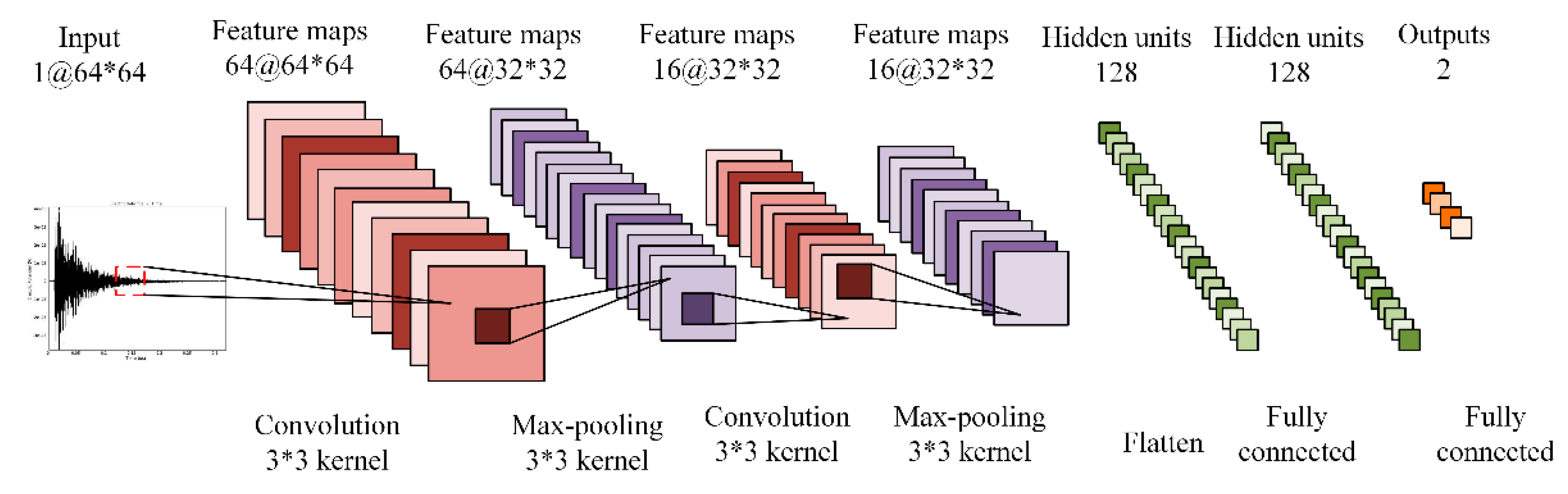
2.2. Convolutional Neural Network

Developed in recent years, CNN has been widely considered as one of efficient pattern recognition methods. Generally, the basic structure of CNN consists of two layers, feature extraction layer and feature mapping layer [39]. In feature extraction layer, each neuron input is connected to the local receptive field of the previous one. Once the local features are extracted, their positional relationship with other features is also determined. In feature mapping layer, each computing layer of the network is composed of multiple feature maps. Each feature map is a plane where the weights of all neurons are equal. The feature mapping structure adopts the ReLU function, a small influence function, as the activation function of the convolution network, to ensure the shifting invariance of the feature map. In addition, since the neurons on one map plane share weights, the number of network free parameters is reduced. Each convolutional layer in the CNN is closely followed by a computational layer for local averaging and quadratic extraction. This unique structure of two-phase feature extraction effectively reduces feature dimensions.
The CNN is mostly composed of multiple convolution layers and pooling layers, which can be subdivided as feature extraction layers, fully-connected layers, and Softmax layers; the feature map first convolutedly calculates with multiple convolution kernels and then is connected to the next layer with bias calculation, activation function, and pooling operation. In the convolution layer, each convolution kernel is convolved with the feature maps of the previous one, and then an output feature map can be obtained through an activation function, which can be expressed as:
H i = σ ( H i 1 × W i + b ) ,
where H i refers to the feature map of the i th layer of the CNN, σ is the activation function, * is the convolution operator, W i is the weight matrix of the i th convolution kernel, and b i is the offset vector of the i th layer. Currently, the main activation functions are tanh, sigmoid, and ReLU.
For the pooling layer, the calculation process can be expressed as:
H i = p o o l i n g ( H i 1 ) .
Pooling represents the pooling operation, which involves averaging, maximization, and random pooling.
In the fully connected layer, the feature maps of the previous layer are processed with the weighted sum method. The output feature map can be attained by the activation function, which can be expressed as:
H i = σ ( H i 1 W i + b i ) .
The training goal of the CNN is to minimize the loss function. When used for classification problems, the loss function uses cross entropy:
J ( θ ) = 1 m i = 1 m y i log ( h θ ( x i ) ) + ( 1 y i ) log ( 1 h θ ( x i ) ) ,
where x i is the i th input, y i is the true value of the i th entry input, m is the number of training samples, and h θ ( x i ) is the predicted value of the i th entry input.
When used for regression problems, the loss function uses the mean square error function:
J ( θ ) = i = 1 m ( ( y i h θ ( x i ) ) 2 m .
In the training process, the gradient descent method is used for model optimization while the back-propagated residual layer by layer updates the parameters (W and b) of each layer in the CNN. Some variations of the gradient descent method include Momentum, Ada Grad, RMS Prop, the stochastic gradient descent algorithm, and the Adam algorithm [40].

2.3. Convolutional Neural Network

Deconvolution, proposed by Zeilor et al. [41], is the process of reconstructing the unknown input by measuring the output and the input. In neural networks, the deconvolution process does not involve learning and is merely used to visualize a trained convolutional network model. The visual filter characteristics obtained by the deconvolution network are similar to the Tokens proposed by Marr in Vision.
Assume that the i th layer input image is y i , which is composed of K 0 channels, y 1 i , y 2 i , , y K 0 i , and c is the channel of the image. The deconvolution operation is expressed as a linear sum of the convolution of K 1 feature maps, Z k i , and filter, f K , c :
k = 1 K 1 Z k i f k , c = y c i .
As for y i :
y i = c = 1 K 0 y c i = c = 1 K 0 k = 1 K 1 Z k i f k , c .
If y c i is an image with N r × N c pixels and the filter size is H × H , then the size of the derived feature map, Z k i , is ( N r + H 1 ) × ( N c + H 1 ) . The loss function can be expressed as:
C 1 ( y i ) = λ 2 c = 1 K 0 | | K = 1 K 1 Z k i f k , c y c i | | 2 2 + k = 1 K 1 | z k i | p ,
where the first term is the mean square error of the reconstructed image and the input image, and the second is the regularization term in the form of the p norm.
In contrast to the CNN, the structure of the deconvolution neural network is mainly composed of a reverse pooling layer and a deconvolution layer. For a complex deep convolutional neural network, through the transformation of several convolution kernels in each layer, it is impossible to know the information automatically extracted by each convolution kernel. Through deconvolution reduction, however, the information can be clearly visualized. The feature maps obtained by each layer are inputted, and then deconvolution is conducted to obtain deconvolution results, which can be used to verify the feature maps extracted by each layer.

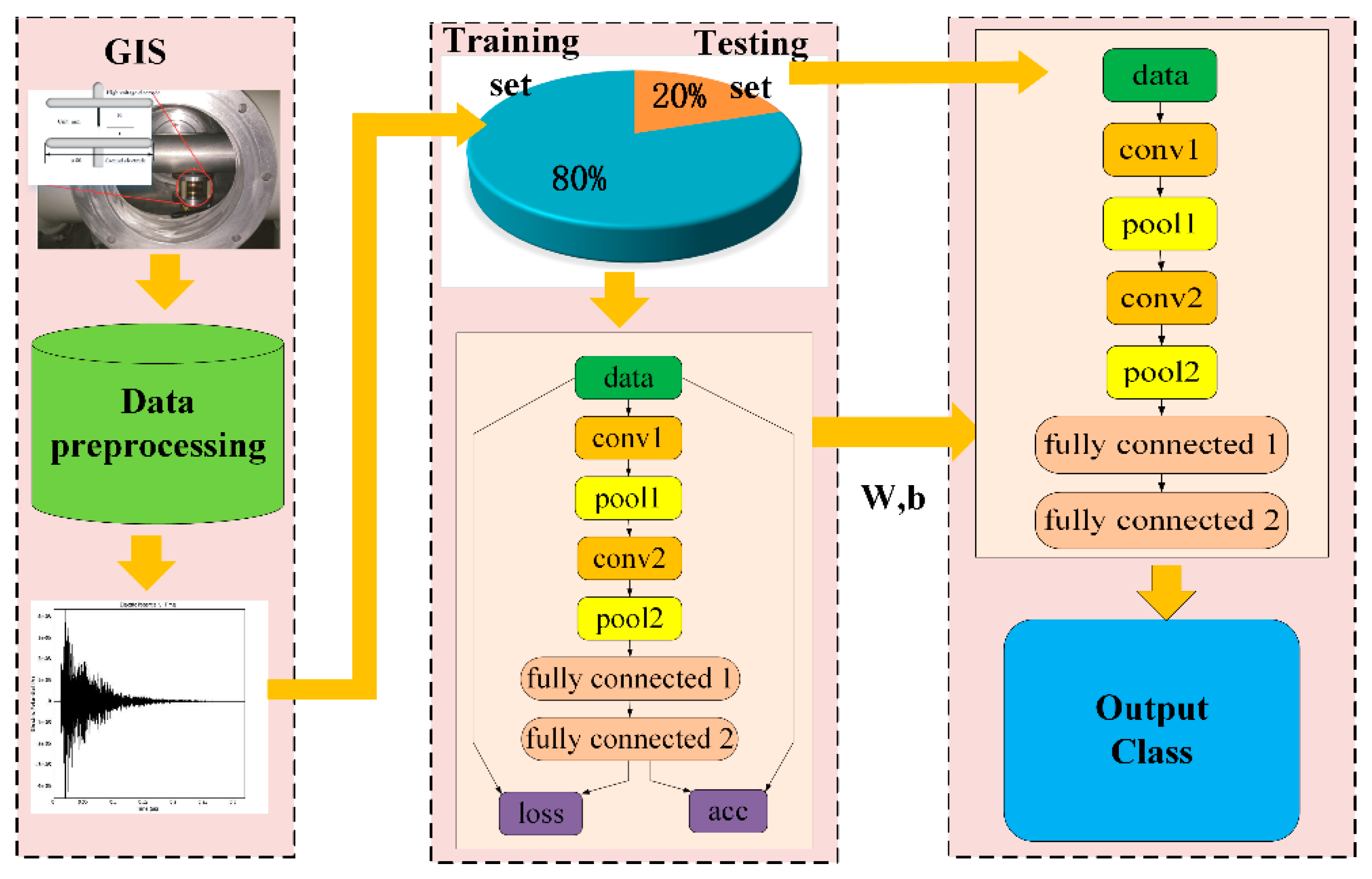
3. GIS PD Pattern Recognition Using Light-Scale Convolutional Neural Network
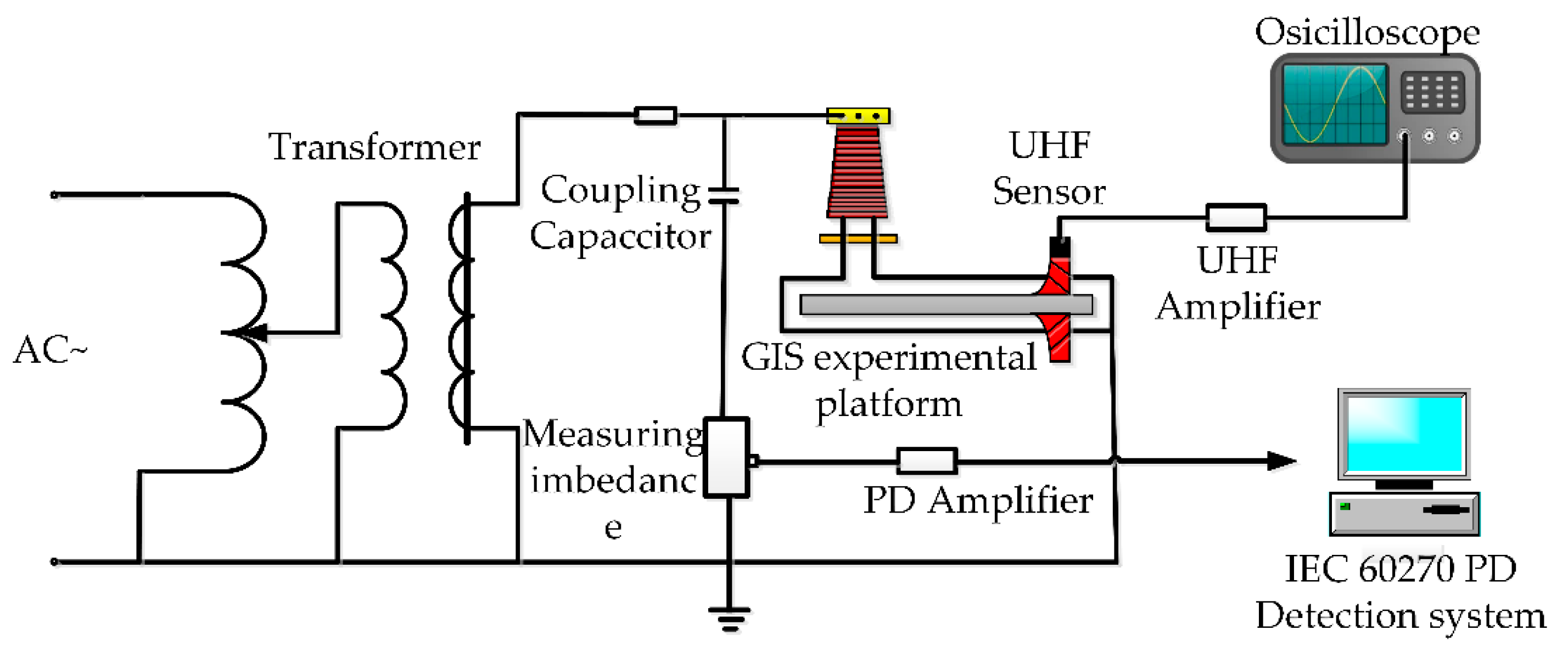
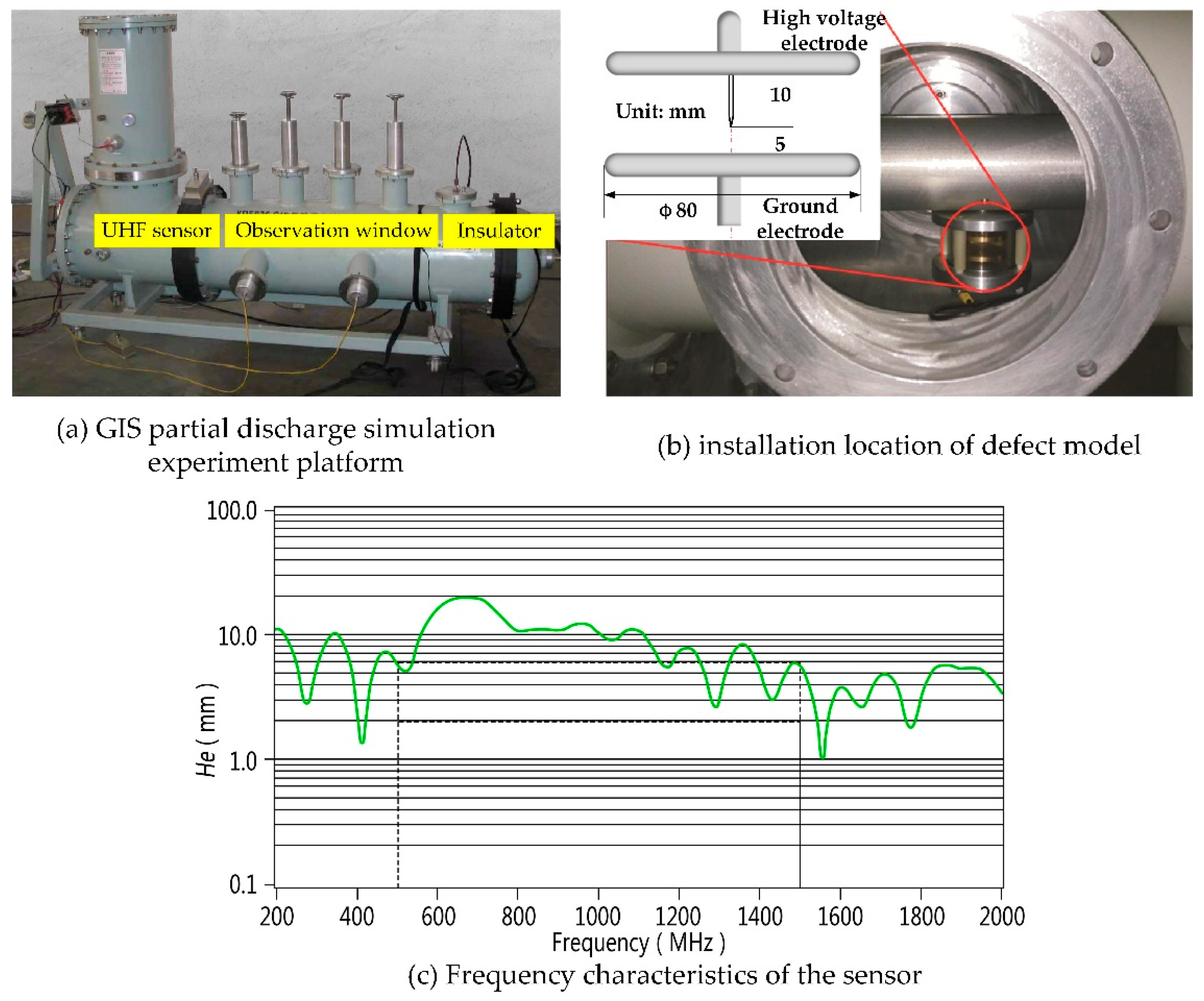
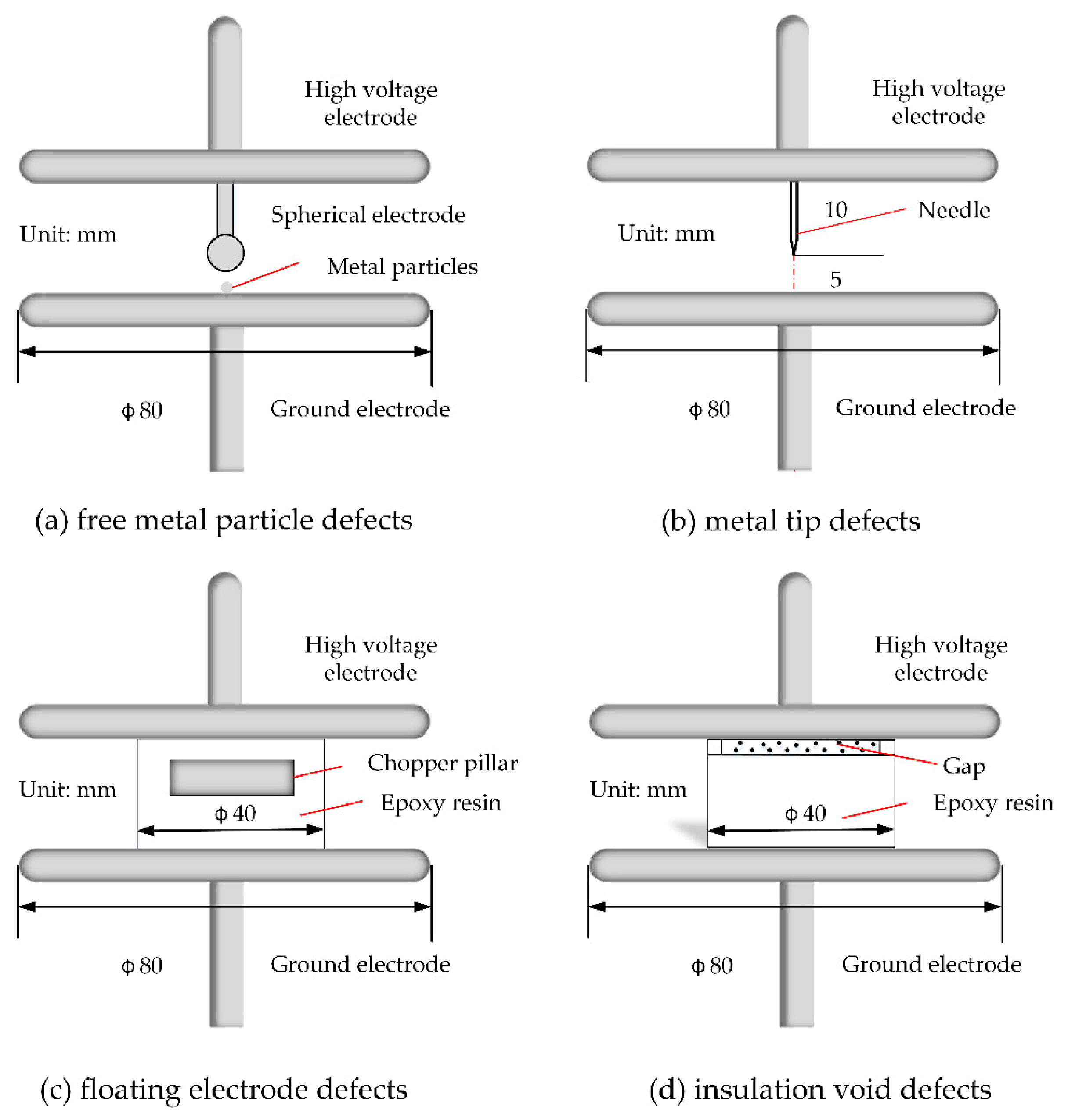
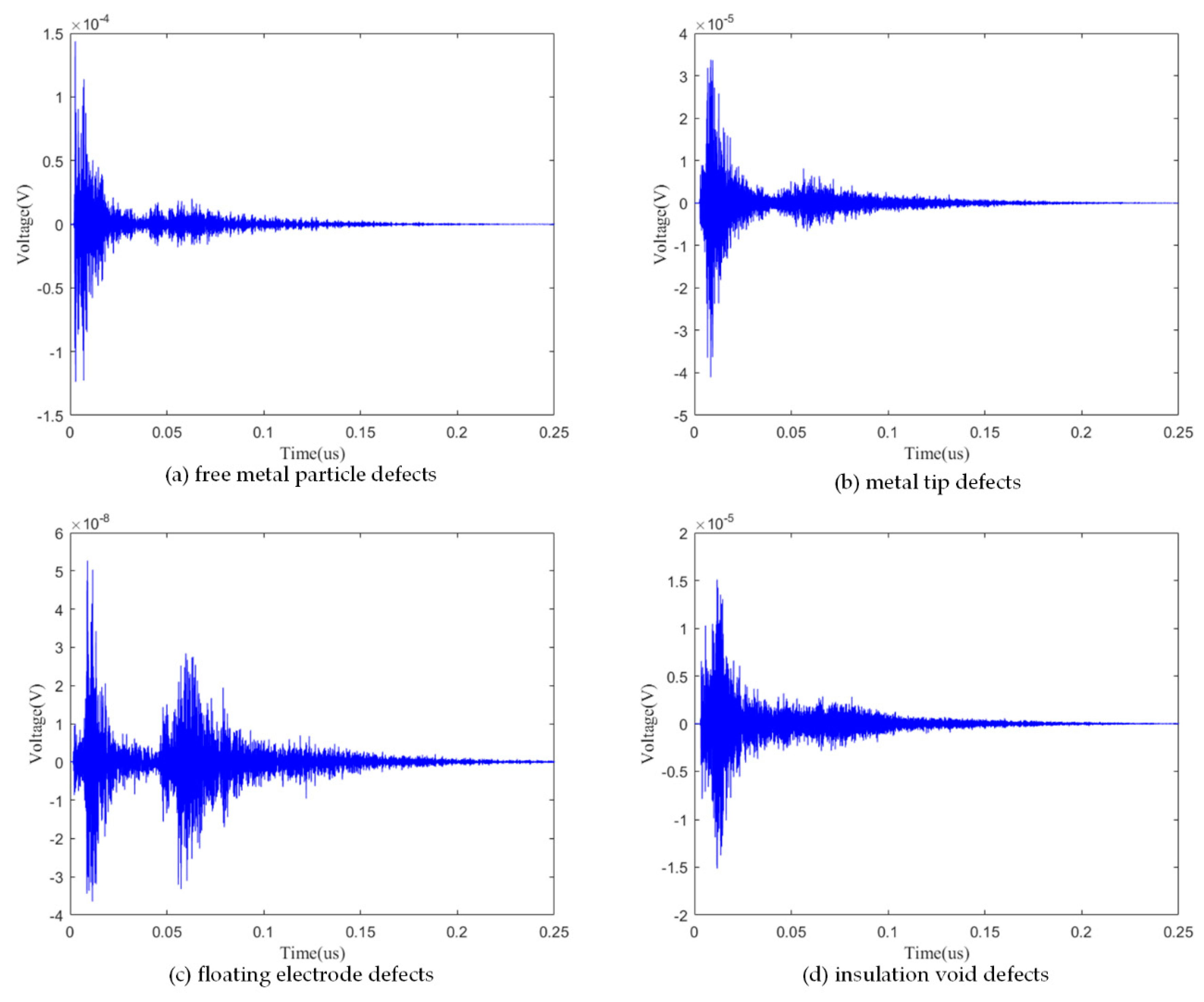
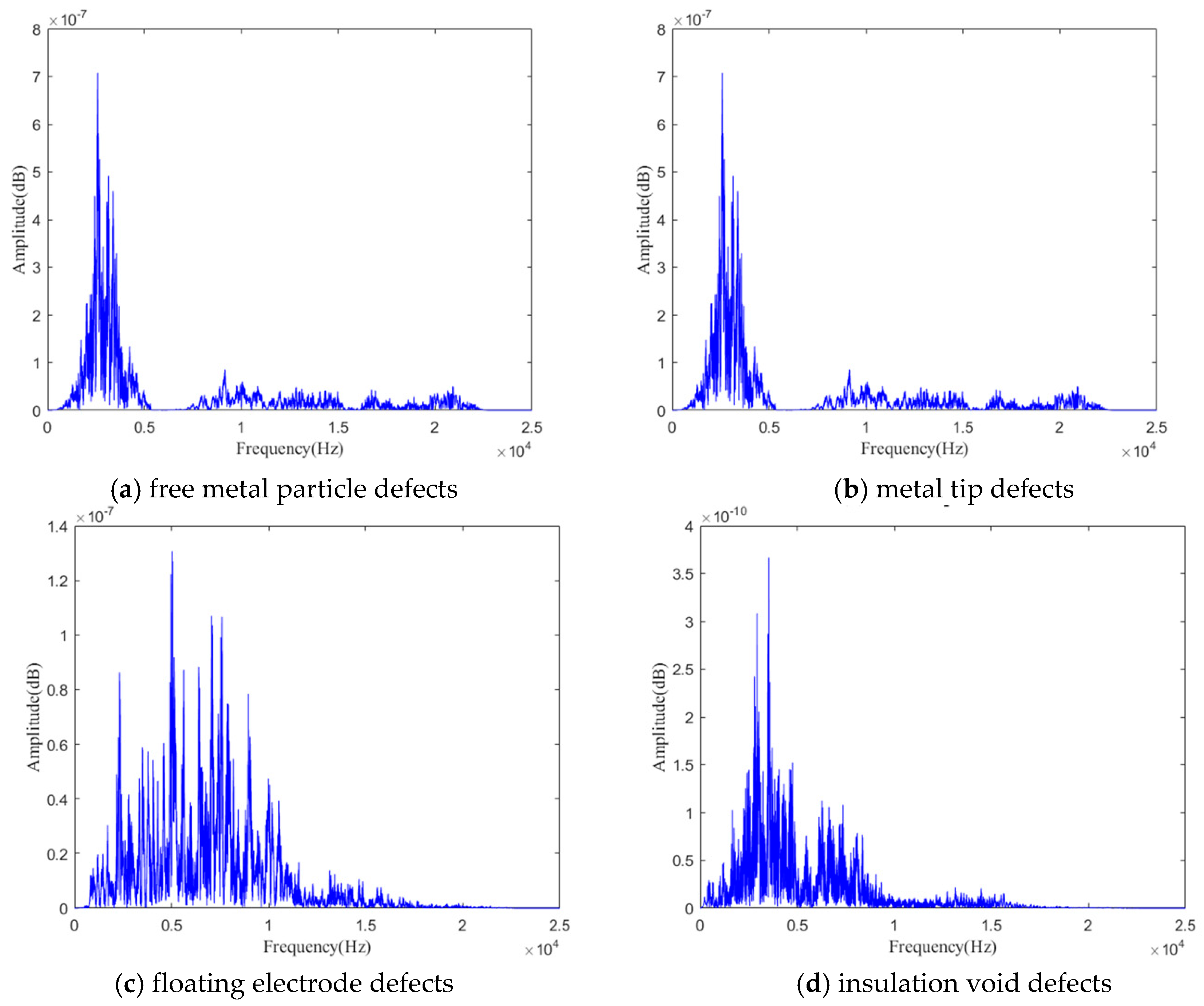
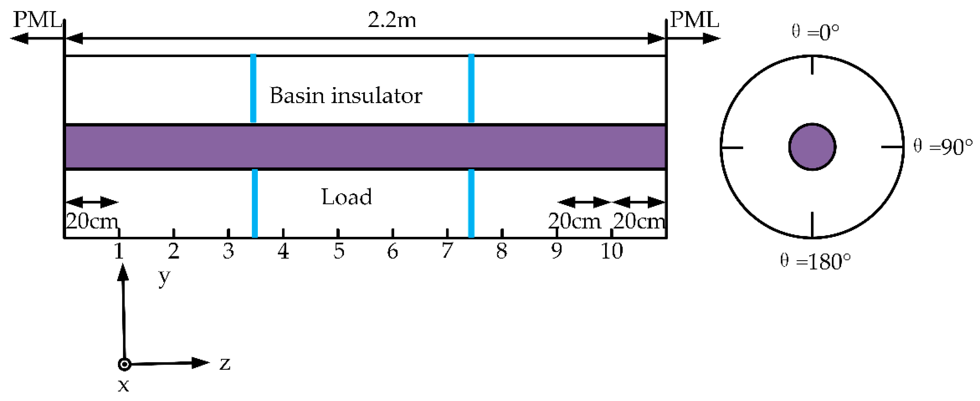
In this paper, the LCNN structure for PD pattern recognition is constructed, which is further clearly shown in Figure 1. This LCNN consists of seven layers in total, namely, two convolutional layers, two pooling layers, two fully connected layers, and one Softmax layer. In the input layer, data are input via a TRPD single-channel banalization image, and converted from 600 × 438 to 64 × 64 by the image downsampling technique. The first convolutional layer consists of 64 3 × 3 convolution kernels, and the second consists of 16 3 × 3 convolution kernels. In the pooling layer, all operations are 3 × 3 maximum pooling, with two strides. Both fully connected layers contain 128 neurons each, and the second fully connected layer is optimized by dropout to avoid overfitting of the model. In the output layer, Softmax is used as a classifier, and one-hot encoding is used to identify four PDs pattern maps. All activation functions in the model are ReLU functions.
The LCNN-based PD pattern recognition process is presented in Figure 2. Specific steps are as follows:
(1) Data preprocessing. The PD time-domain map is shrunk from 600 × 438 to 64 × 64 by image downsampling.
(2) Data enhancement. The CVAE is used to randomly select 20% of the data as training data for image generation to improve the generalization ability of the model.
(3) Model training. The model training uses a back-propagated algorithm and a stochastic gradient descent algorithm. In the pooling layer, the data are normalized. In the fully connected layer, the dropout method is adopted.
(4) Model testing. Model testing is conducted with 20% of the remaining image to verify the generalization ability, fault recognition accuracy, and testing time.
(5) Model visualization. TensorBoard and a deconvolution neural network are used to achieve full visualization of the whole training process and feature extraction process, which solves the “black-box” problem in CNNs.

4. Data Acquisition

Four typical GIS PD defects were selected for pattern recognition and fault classification: Free metal particle defects, metal tip defects, floating electrode defects, and insulation void defects. A schematic of the experiment is shown in Figure 3.
In the experiment, the rated voltage of the transformer was 250 kV and the rated capacity was 50 kVA. The UHF sensor was composed of an amplifier, a high-pass filter, a detector, and a shielding case and its detection frequency band was 300 to 2000 MHz. The working bandwidth of the amplifier was 300 to 1500 MHz, and the amplifier gain was 40 dB. The sensor had a mean effective height of He = 10.2 mm over the frequency range of 500 to 1500 MHz, as shown in Figure 4c. The oscilloscope single-channel sampling rate was 10 GS/s, and the analogue bandwidth was 2 GHz. The experimental device and defect model installation location, defect models, TRPD PD waveforms, and frequency spectrum maps are respectively shown in Figure 4, Figure 5, Figure 6 and Figure 7.
To more thoroughly capture GIS PD characteristics, following [42,43,44,45,46], the four typical kinds of GIS PD signals were simulated with the finite-difference time-domain (FDTD) method. The FDTD method, introduced by Yee in 1966, is a computational method to model electromagnetic wave propagation and interactions with the properties of materials through FDTD software [47,48]. The simulation model is shown in Figure 8. The center conductor and the tank were, respectively, 120 and 400 mm in diameter, and the tank wall was 10 mm in thickness and 2.2 m in length.
The four types of defect simulation models are shown in Figure 9. Let us consider metal tip defects as an example. A metal needle of 30 mm in length was instilled on a high-voltage conductor as an excitation source to simulate an insulation defect. Referring to the discharge signals and experimental conclusions measured by other scholars in actual discharge tests, the signal data and Gaussian pulses under different defect conditions were used as the excitation source of the fault simulation part of this article. The Gaussian pulse with a broadband of −30 dB attenuation at −3 GHz was added to the needle as a PD current pulse [45,46]. To guarantee consistency with the actual situation, the needle and current were placed perpendicular to the conductor surface in the y direction, and a seven-layer perfect matching layer (PML) of the two terminals was applied to match the impedance of the adjacent medium, without the reflection and refraction of the GIS end taken into account. The cavity boundaries in the other two directions were set in the same way as the y axis. Furthermore, with regard to loss at the conductor walls, an ideal conductor was used for the high-voltage conductors and cavities. The relative dielectric constant of SF6 filled in the GIS cavity is 1.00205, and the density was set as 23.7273 kg/m3 under a pressure of 0.4 MPa (absolute). The relative magnetic permeability and electrical conductivity were 1 and 1.1015 × 10⁻⁵ S/m, respectively. The highest frequency of the calculation was 3 GHz and the cell size was set as 10 mm × 10 mm × 10 mm. The simulation time was 250 ns and the time step was 9.661674 × 10⁻⁶ us. The simulation conditions for the other three defects were the same.
For free metal particle defects, 10-mm-long metal particles were placed in the outer shell of the bus bar, which corresponds to the conditions of the experiment performed using the actual GIS. For floating electrode defects, the inner side of the ring, having a diameter of 101 mm, was tangent to the high-voltage conductor to simulate the floating electrode. For air gap defects, a 3-mm air gap was reserved in the basin insulator model to simulate the air gap in the GIS. During the simulation process, the random variation of the sensor (test point) is adopted and the defect position is relatively unchanged to simulate the randomness of the local partial discharge. The measurement points are set every 100 mm, and each measurement point is measured at intervals of 0–180° relative to the defect distribution every 15°. The FDTD simulation waveforms and frequency spectrum of four kinds of defects are shown in Figure 10 and Figure 11. As can be seen from Figure 6, Figure 7, Figure 10 and Figure 11, there are certain differences in the waveform and spectrum between the experimental data and the simulated data, mainly reflected in the changes of amplitude and phase. However, for the same type of defect, because the simulation excitation source comes from the experimental process, the simulation and experimental data show the same trend in the entire waveform or spectrum change, which is obviously different from other types of defects.

5. Results and Analysis

In this paper, 3200 TRPD data consisting of 1200 experimental data and 2000 FDTD simulation data were used for PD pattern classification. In total, 80% of data were randomly selected for training, and the remaining 20% were for testing. We trained our model with TensorFlow on a machine equipped with one 8 GB GeForce RTX 2060 GPU. Additionally, we chose Anaconda as our Python package manager and its distribution of TensorFlow. Moreover, we developed all our programs in PyCharm IDE.

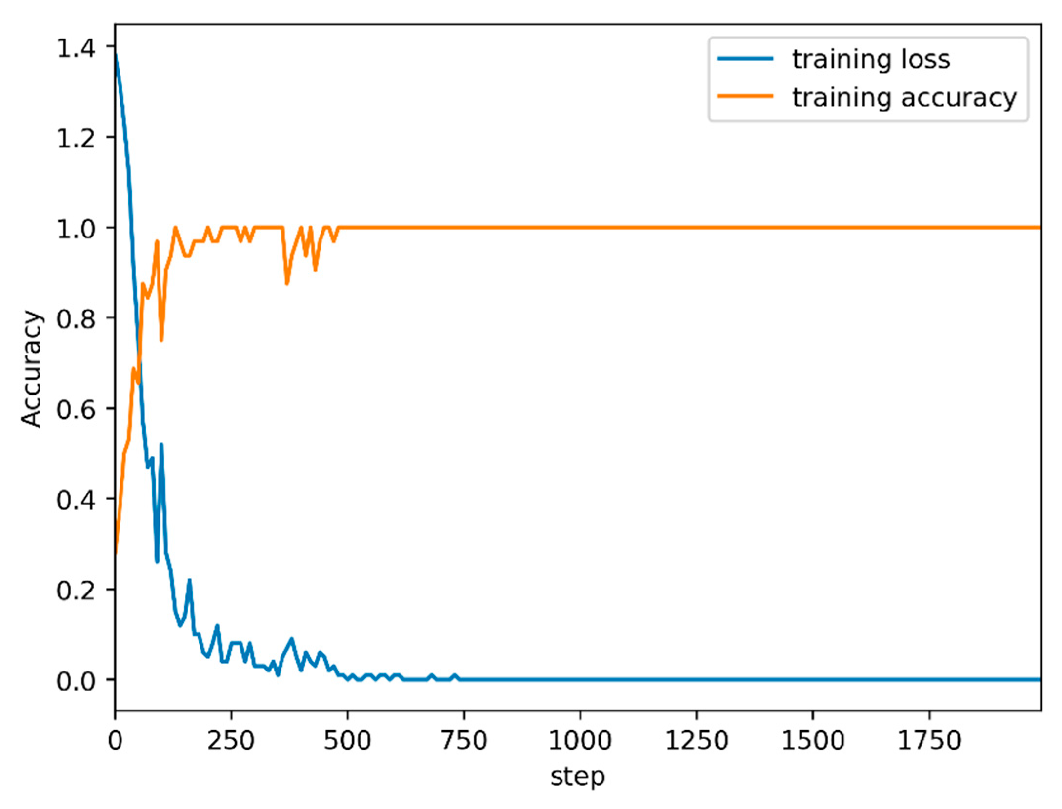
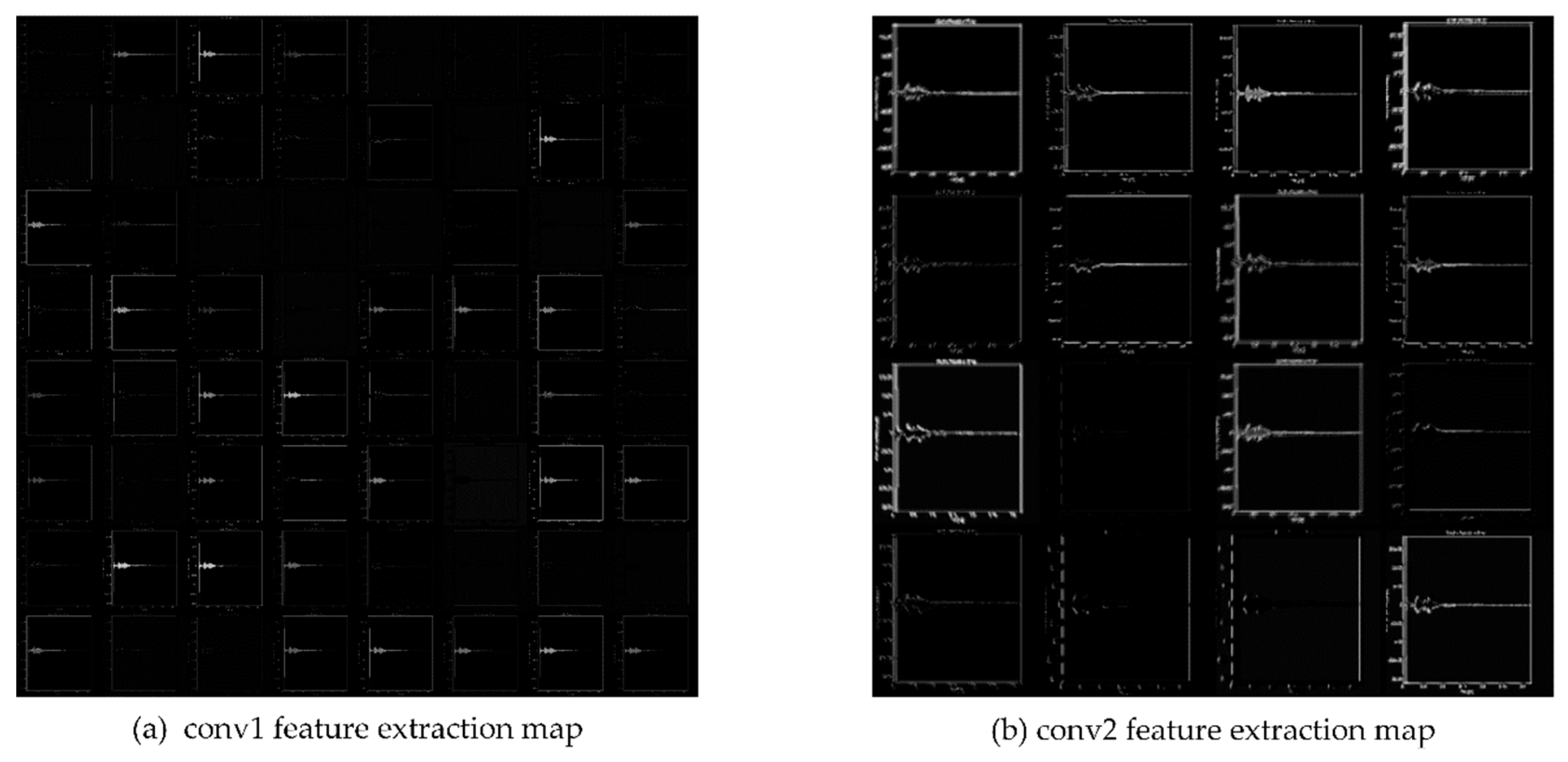
5.1. Model Training and Visualization

The CNN is regarded as a “black-box” model. Thus, in this paper, to visualize the entire training and feature extraction process, a TensorBoard-integrated deconvolution neural network method was adopted. Through the visualization, the features extracted from each layer of the model can be easily observed. Meanwhile, use of the method can also help in monitoring the whole training process and then evaluating the overfitting problem of the model. The model training process was visualized by TensorBoard, and the visualized results of the loss function and training accuracy curves are shown in Figure 10. It can be seen from Figure 12 that the loss function decreases with increasing training, and the rate of the decreasing speed drops with the increase of the training. The loss function fluctuates around 0.1 at the 500th training step, fluctuates around 0 at the 1000th training step, and drops to 0 after 750 training steps. The trend of the training accuracy is exactly opposite to that of the loss function, but they share the same trend of change rate. Thus, the model performs quite well on the training set.
Visualization of the automatic feature extraction in the CNN is presented in Figure 13. Obviously, the learned convolution filter is relatively smooth in space, which is the result of sufficient training. Moreover, the feature visualization results indicate that the features extracted by the CNN are sensitive to time. In the initial features extracted, most are in the form of waveform contours. In the later feature maps, these waveform features gradually coalesced, and, in the final maps, the initial waveform features can be seen much more clearly.

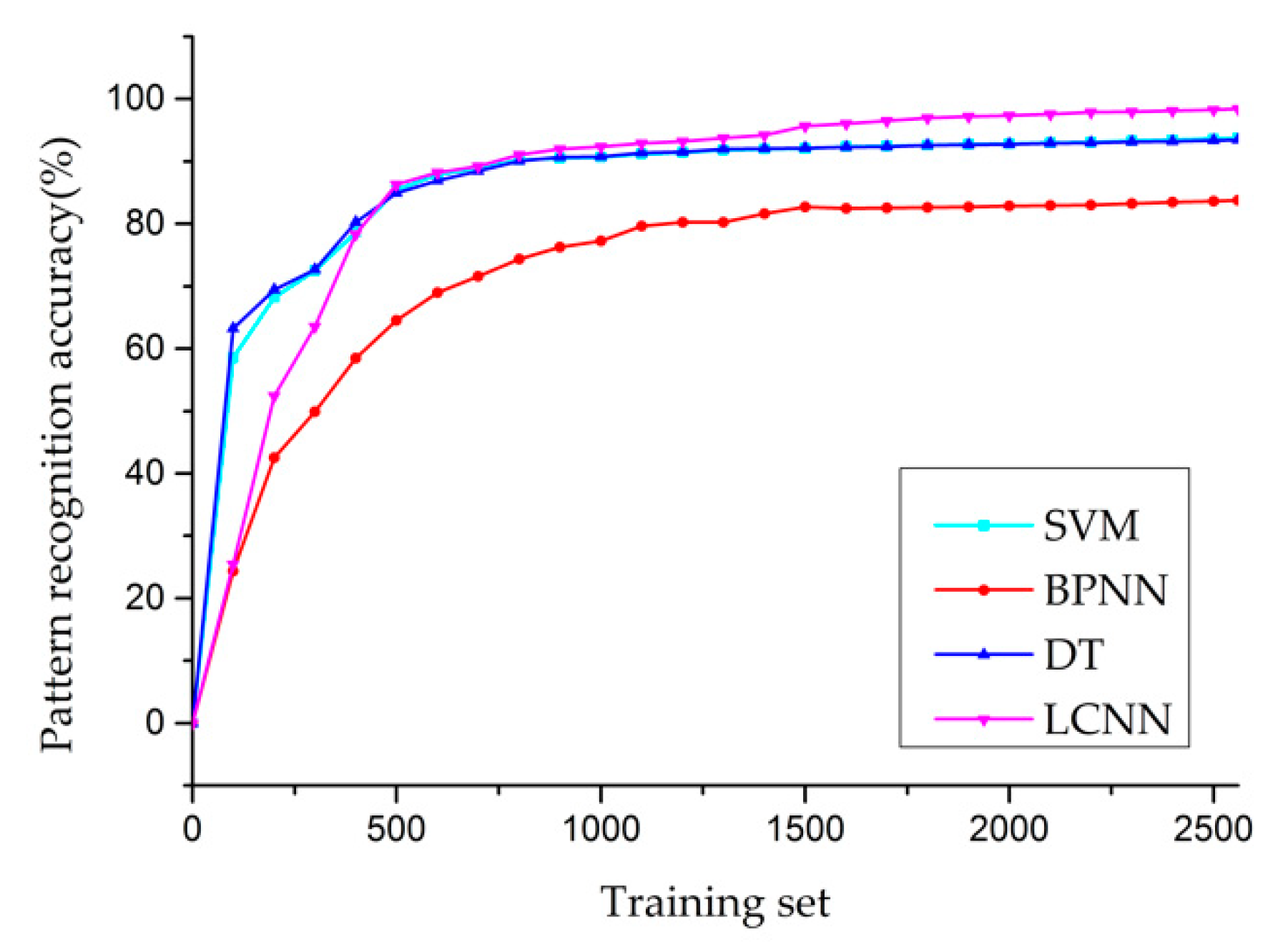
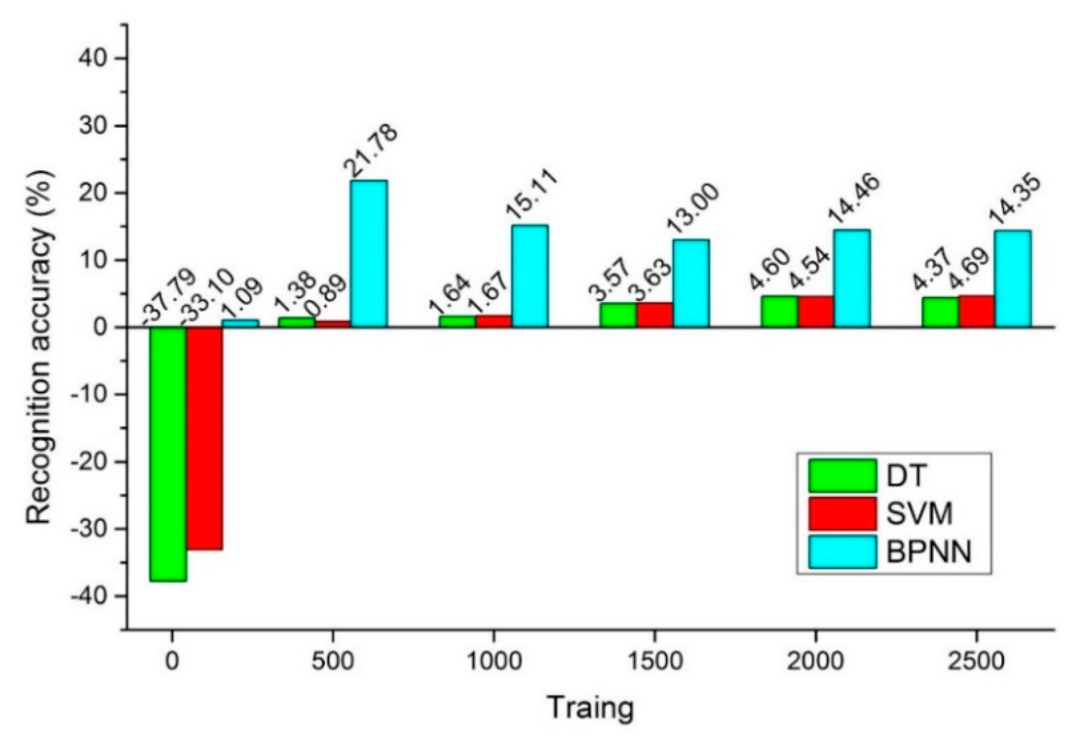
5.2. Accuracy Analysis of Pattern Recognition

To effectively assess the recognition accuracy of the model, 2560 groups of 3200 TRPD maps covering four major defects—free metal particle defects (M-type defects), metal tip defects (N-type defects), suspended electrode defects (O-type defects), and insulation void defects (P-type defects)—were used for model testing. Support vector machine (SVM), decision trees (DT), BP neural network (BPNN), LeNet5, AlexNet, VGG16, and LCNN models were used for GIS PD pattern recognition. The recognition results are given in Table 1 (with reference to [49], the maximum value, root mean square deviation, standard deviation, skewness, kurtosis, and the peak-to-peak value were selected as feature parameters [49]).
As can be seen in Table 1, the overall recognition rate of the LCNN reached 98.13% of 640 testing sets while the rates of SVM, BPNN, DT, LeNet5, AlexNet, and VGG16 were, respectively, 93.76%, 83.78%, 93.44%, 75.04%, 90.63%, and 86.41%. The recognition rate of the LCNN is significantly higher than that of the traditional machine learning methods and of the deep learning method. The recognition rate of different recognition methods varies significantly in identifying different defect types. In general, the LCNN outperforms the other methods in defect recognition, whereas LeNet5 has the lowest recognition rate. The reason why the recognition rates of the traditional machine learning methods and LeNet5 are low is that the features are underutilized; AlexNet and VGG16 have low rates because of their inability to address the vanishing gradient during model training, through the transfer learning, the recognition rate of both is improved, but the overall recognition rate is limited by the size of the data set. All the methods except AlexNet and VGG16, however, have much greater difficulty in identifying insulator insulation void defects. This is because the internal defects of the insulator mainly entail minor gaps in the molding resin or voids in the layered region between the insulating material and the metal insert, and, with the long-time accumulation of electric field, the instability of the PD under such defects leads to low recognition accuracy [50].
To further compare the performance of the LCNN and traditional machine learning methods, training sets of different sample sizes were used for model training. The recognition accuracy curves for different algorithms for PD pattern classification are shown in Figure 14. As can be seen from Figure 14, the LCNN demonstrates the largest variation in accuracy before the number of training samples reaches 500. When the number of training samples are fewer than 500, both the SVM and DT methods outperform the LCNN. With >500 samples, however, the LCNN is significantly superior to the other traditional machine learning methods. Therefore, generally, the LCNN performs the best, followed by the SVM and DT, both of which have relatively high recognition accuracy for small-sized samples. The BPNN has the worst performance. Figure 15 reports the improvement in recognition accuracy of the LCNN for different training samples compared to traditional machine learning algorithms.
It can be seen from Figure 15 that, when the number of training samples is 100, compared with DT, SVM, and BPNN methods, improvement in recognition accuracy of the LCNN is −37.79%, −33.1%, and 1.09%, respectively. The recognition accuracies of the SVM and DT methods are significantly higher than that of the LCNN. Therefore, for small samples, traditional machine learning methods possess evident advantages over the LCNN. When the training data set reaches 500, the recognition accuracy of the LCNN, improves by 1.38%, 0.89%, and 21.78%, respectively, which means that the LCNN has begun to demonstrate its advantages in recognition accuracy. When the sample size of training data reaches 2500, the accuracy of the LCNN improves by 4.37%, 4.69%, and 14.35%, respectively. At this point, the LCNN significantly outperforms traditional machine learning methods. With the increase of the training data sets, the LCNN method demonstrates growing advantages over traditional machine learning methods in recognition accuracy. Therefore, the overall performance of the LCNN is significantly better than that of machine learning methods. In the context of big data and the ubiquitous-power IoT, the LCNN has broad application prospects.

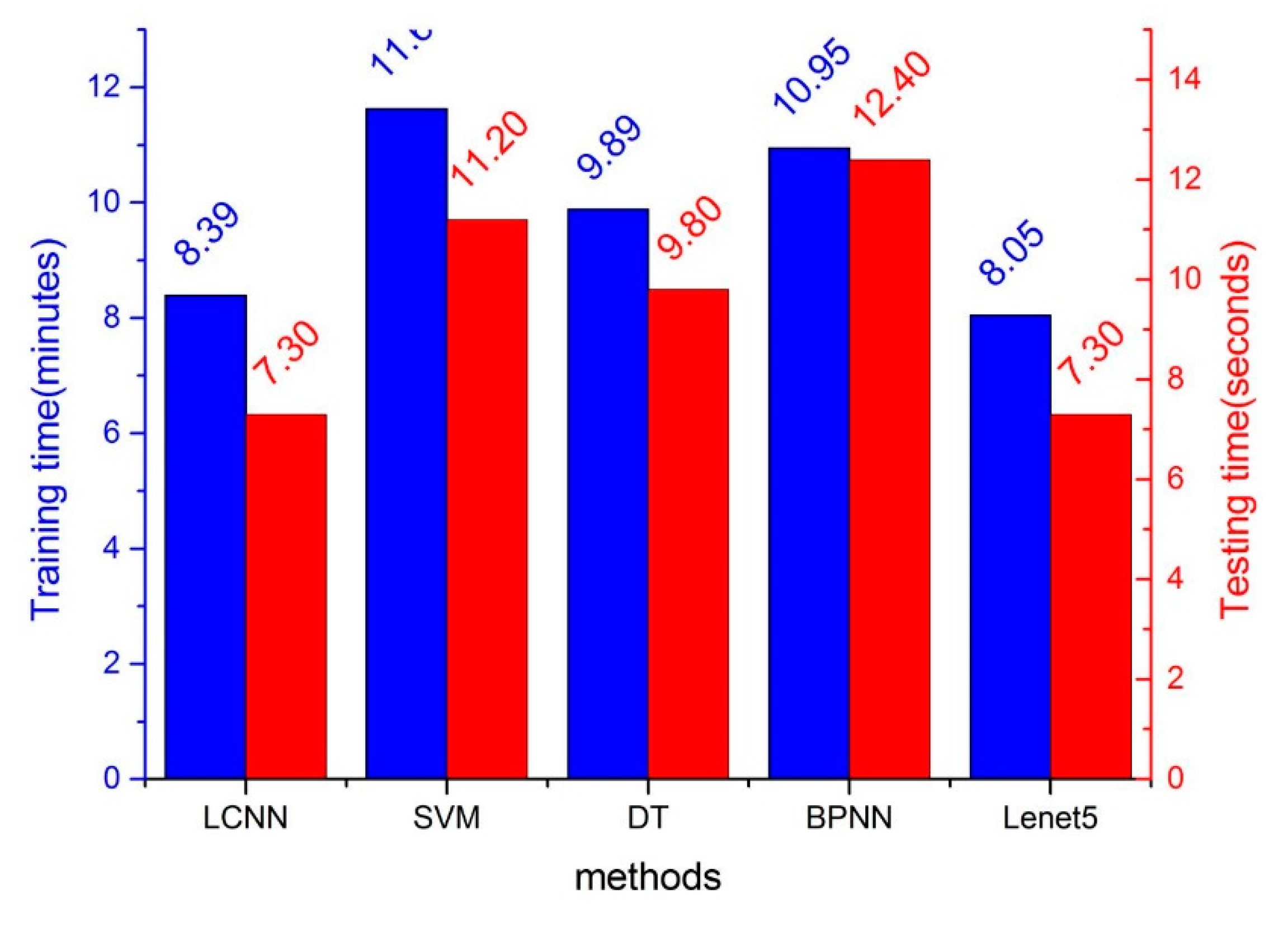
5.3. Model Time Analysis

The length of time spent in model training and testing directly determines whether the model can be applied under the ubiquitous-power IoT. The current testing time cannot meet the requirement of quick, real-time processing under online monitoring of the ubiquitous-power IoT. The length of training time affects the updating ability of the model. It is difficult to update the model for better accuracy when much more training samples are acquired to form a larger historical knowledge database. To verify the temporal advantages of the LCNN model proposed in this paper, the training data of the SVM, DT, and BPNN were used for comparison. Figure 16 shows the training time and testing time distribution of different models based on the 3200 groups of the TRPD data set.
In Figure 16, the LCNN training time is 8.39 min, 11.63 min with the SVM, 9.89 min with the DT, and 10.95 min with the BPNN. The LCNN testing time is 7.3 s < 11.2 s with the SVM, 9.8 s with the DT, and 12.4 s with the BPNN. Therefore, the LCNN model has an evident advantage in training time and testing time. One of the main reasons why traditional machine learning models consume much more time is that they take a massive amount of time to extract features.
By comparison with traditional machine learning methods, such as the SVM, DT, and BPNN, it can be seen that the LCNN proposed in this paper demonstrates obvious advantages over other methods in training time and testing time. The shorter testing time makes it possible to handle fault signals quickly and in time, which lays a solid foundation for t-fault diagnoses of GIS PD in the context of the ubiquitous-power IoT and big data.

6. Conclusions

In this paper, an LCNN model was proposed for GIS PD pattern recognition. In the TRPD mode, the light-scale model mitigates the dependence of traditional machine learning on expert experience and avoids the risk that the depth model cannot be trained because of the vanishing gradient. It also maximizes the simulation of various working conditions of PD and makes full use of the time-domain waveform characteristics of PD. Therefore, it effectively improves the accuracy of the model and reduces both training time and test time, making it more applicable to the ubiquitous-power IoT. The following conclusions can be drawn:
(1) Visualization of the entire training and automatic feature extraction process of the LCNN can be realized by the deconvolution neural network integrated with TensorBoard. As a result, the “black-box” problem of the CNN is solved. The feasibility of LCNN was verified by a visual training process, and the features were visually displayed.
(2) LCNN has superior feature capture capability for GIS PD signals and effectively implements GIS PD pattern recognition. Based on TRPD, the overall recognition rate of the LCNN reached 98.13%, while rates of the SVM, BPNN, DT, LeNet5, AlexNet, and VGG16 were 93.76%, 83.78%, 93.44%, 75.04%, 90.63%, and 86.41%, respectively. With the increase of the number of samples, the LCNN demonstrates more advantages, which make it much more suitable for application to big data and the ubiquitous-power IoT.
(3) Banalization and image downsampling considerably alleviated the burden of time consumption for model training. By comparison with traditional machine learning methods, the TRPD-based LCNN demonstrates significant advantages over other methods in training time and testing time. It can not only accomplish quick, real-time online monitoring of fault signals but also rapidly update the model after resetting the fault knowledge base.

Author Contributions

Y.W. and J.Y. conceived and designed the experiments; J.L. provided the experimental data; Y.W. wrote the paper; Z.Y. modified the code of the paper; T.L. revised the contents and reviewed the manuscript; Y.Z. provided the simulation data.

Funding

This research received no external funding.

Acknowledgments

Special thanks to NVIDIA graphic processing unit and XFDTD software for technical support. Thanks to Anhui Electric Power Research Institute for data support.

Conflicts of Interest

The authors declare no conflict of interest.

References

  1. Khan, Q.; Refaat, S.S.; Abu-Rub, H.; Toliyat, H.A. Partial discharge detection and diagnosis in gas insulated switchgear: State of the art. IEEE Electr. Insul. Mag. 2019, 35, 16–33. [Google Scholar] [CrossRef]
  2. Gao, W.; Ding, D.; Liu, W. Research on the typical partial discharge using the UHF detection method for GIS. IEEE Trans. Power Deliv. 2011, 26, 2621–2629. [Google Scholar] [CrossRef]
  3. Stone, G.C. Partial discharge diagnostics and electrical equipment insulation condition assessment. IEEE Trans. Dielectr. Electr. Insul. 2005, 12, 891–904. [Google Scholar] [CrossRef]
  4. Niu, X.; Shao, S.; Xin, C.; Zhou, J.; Guo, S.; Chen, X.; Qi, F. Workload Allocation Mechanism for Minimum Service Delay in Edge Computing-Based Power Internet of Things. IEEE Access 2019, 7, 83771–83784. [Google Scholar] [CrossRef]
  5. Hu, W.; Yao, W.; Hu, Y.; Li, H. Selection of Cluster Heads for Wireless Sensor Network in Ubiquitous Power Internet of Things. Int. J. Comput. Commun. Control 2019, 14, 344–358. [Google Scholar] [CrossRef]
  6. Yao, R.; Hui, M.; Li, J.; Bai, L.; Wu, Q. A New Discharge Pattern for the Characterization and Identification of Insulation Defects in GIS. Energies 2018, 11, 971. [Google Scholar] [CrossRef] [Green Version]
  7. Han, X.; Li, J.; Zhang, L.; Pang, P.; Shen, S. A Novel PD Detection Technique for Use in GIS Based on a Combination of UHF and Optical Sensors. IEEE Trans. Instrum. Meas. 2019, 68, 2890–2897. [Google Scholar] [CrossRef]
  8. Okubo, H.; Hayakawa, N. A novel technique for partial discharge and breakdown investigation based on current pulse waveform analysis. IEEE Trans. Dielectr. Electr. Insul. 2005, 12, 736–744. [Google Scholar] [CrossRef]
  9. Li, T.; Rong, M.; Zheng, C.; Wang, X. Development simulation and experiment study on UHF partial discharge sensor in GIS. IEEE Trans. Dielectr. Electr. Insul. 2012, 19, 1421–1430. [Google Scholar] [CrossRef]
  10. Si, W.; Li, J.; Li, D.; Yang, J.; Li, Y. Investigation of a comprehensive identification method used in acoustic detection system for GIS. IEEE Trans. Dielectr. Electr. Insul. 2010, 17, 721–732. [Google Scholar] [CrossRef]
  11. Li, J.; Han, X.; Liu, Z.; Yao, X. A novel GIS partial discharge detection sensor with integrated optical and UHF methods. IEEE Trans. Power Deliv. 2016, 33, 2047–2049. [Google Scholar] [CrossRef]
  12. Tang, J.; Liu, F.; Zhang, X.; Meng, Q.; Zhou, J. Partial discharge recognition through an analysis of SF6 decomposition products part 1: Decomposition characteristics of SF 6 under four different partial discharges. IEEE Trans. Dielectr. Electr. Insul. 2012, 19, 29–36. [Google Scholar] [CrossRef]
  13. Gao, W.; Ding, D.; Liu, W.; Huang, X. Investigation of the Evaluation of the PD Severity and Verification of the Sensitivity of Partial-Discharge Detection Using the UHF Method in GIS. IEEE Trans. Power Deliv. 2013, 29, 38–47. [Google Scholar]
  14. Umamaheswari, R.; Sarathi, R. Identification of partial discharges in gas-insulated switchgear by ultra-high-frequency technique and classification by adopting multi-class support vector machines. Electr. Power Compon. Syst. 2011, 39, 1577–1595. [Google Scholar] [CrossRef]
  15. Hirose, H.; Hikita, M.; Ohtsuka, S.; Tsuru, S.-I.; Ichimaru, J. Diagnosis of electric power apparatus using the decision tree method. IEEE Trans. Dielectr. Electr. Insul. 2008, 15, 1252–1260. [Google Scholar] [CrossRef]
  16. Deng, R.; Zhu, Y.; Liu, X.; Zhai, Y. Multi-source Partial Discharge Identification of Power Equipment Based on Random Forest. In The IOP Conference Series: Earth and Environmental Science; IOP Publishing: Qingdao, China, 2019; Volume 17, p. 062039. [Google Scholar]
  17. Su, M.-S.; Chia, C.-C.; Chen, C.-Y.; Chen, J.-F. Classification of partial discharge events in GILBS using probabilistic neural networks and the fuzzy c-means clustering approach. Int. J. Electr. Power Energy Syst. 2014, 61, 173–179. [Google Scholar] [CrossRef]
  18. Tang, J.; Wang, D.; Fan, L.; Zhuo, R.; Zhang, X. Feature parameters extraction of GIS partial discharge signal with multifractal detrended fluctuation analysis. IEEE Trans. Dielectr. Electr. Insul. 2015, 22, 3037–3045. [Google Scholar] [CrossRef]
  19. Li, X.; Wang, X.; Xie, D.; Wang, X.; Yang, A.; Rong, M. Time–frequency analysis of PD-induced UHF signal in GIS and feature extraction using invariant moments. IET Sci. Meas. Technol. 2017, 12, 169–175. [Google Scholar] [CrossRef]
  20. Kawada, M.; Tungkanawanich, A.; Kawasaki, Z.-I.; Matsu-Ura, K. Detection of wide-band EM signals emitted from partial discharge occurring in GIS using wavelet transform. IEEE Trans. Power Deliv. 2000, 15, 467–471. [Google Scholar] [CrossRef] [Green Version]
  21. Gu, F.-C.; Chang, H.-C.; Kuo, C.-C. Gas-insulated switchgear PD signal analysis based on Hilbert-Huang transform with fractal parameters enhancement. IEEE Trans. Dielectr. Electr. Insul. 2013, 20, 1049–1055. [Google Scholar]
  22. Shang, H.; Lo, K.; Li, F. Partial discharge feature extraction based on ensemble empirical mode decomposition and sample entropy. Entropy 2017, 19, 439. [Google Scholar] [CrossRef] [Green Version]
  23. Dai, D.; Wang, X.; Long, J.; Tian, M.; Zhu, G.; Zhang, J. Feature extraction of GIS partial discharge signal based on S-transform and singular value decomposition. IET Sci. Meas. Technol. 2016, 11, 186–193. [Google Scholar] [CrossRef]
  24. Candela, R.; Mirelli, G.; Schifani, R. PD recognition by means of statistical and fractal parameters and a neural network. IEEE Trans. Dielectr. Electr. Insul. 2000, 7, 87–94. [Google Scholar] [CrossRef]
  25. Xue, J.; Zhang, X.-L.; Qi, W.-D.; Huang, G.-Q.; Niu, B.; Wang, J. Research on a method for GIS partial discharge pattern recognition based on polar coordinate map. In Proceedings of the 2016 IEEE International Conference on High Voltage Engineering and Application (ICHVE), Chengdu, China, 19–22 September 2016; pp. 1–4. [Google Scholar]
  26. Li, L.; Tang, J.; Liu, Y. Partial discharge recognition in gas insulated switchgear based on multi-information fusion. IEEE Trans. Dielectr. Electr. Insul. 2015, 22, 1080–1087. [Google Scholar] [CrossRef]
  27. Piccin, R.; Mor, A.R.; Morshuis, P.; Girodet, A.; Smit, J. Partial discharge analysis of gas-insulated systems at high voltage AC and DC. IEEE Trans. Dielectr. Electr. Insul. 2015, 22, 218–228. [Google Scholar] [CrossRef]
  28. Hao, L.; Lewin, P.L. Partial discharge source discrimination using a support vector machine. IEEE Trans. Dielectr. Electr. Insul. 2010, 17, 189–197. [Google Scholar] [CrossRef]
  29. Blufpand, S.; Mor, A.R.; Morshuis, P.; Montanari, G.C. Partial discharge recognition of insulation defects in HVDC GIS and a calibration approach. In Proceedings of the 2015 IEEE Electrical Insulation Conference (EIC), Seattle, WA, USA, 7–10 June 2015; pp. 564–567. [Google Scholar]
  30. Li, G.; Wang, X.; Li, X.; Yang, A.; Rong, M. Partial discharge recognition with a multi-resolution convolutional neural network. Sensors 2018, 18, 3512. [Google Scholar] [CrossRef] [Green Version]
  31. Song, H.; Dai, J.; Sheng, G.; Jiang, X. GIS partial discharge pattern recognition via deep convolutional neural network under complex data source. IEEE Trans. Dielectr. Electr. Insul. 2018, 25, 678–685. [Google Scholar] [CrossRef]
  32. Li, G.; Rong, M.; Wang, X.; Li, X.; Li, Y. Partial discharge patterns recognition with deep Convolutional Neural Network. In Proceedings of the Condition Monitoring and Diagnosis, Xi’an, China, 25–28 September 2016; pp. 324–327. [Google Scholar]
  33. Wan, X.; Song, H.; Luo, L.; Li, Z.; Sheng, G.; Jiang, X. Pattern Recognition of Partial Discharge Image Based on One-dimensional Convolutional Neural Network. In Proceedings of the 2018 Condition Monitoring and Diagnosis (CMD), Perth, WA, Australia, 23–26 September 2018; pp. 1–4. [Google Scholar]
  34. Nguyen, M.-T.; Nguyen, V.-H.; Yun, S.-J.; Kim, Y.-H. Recurrent neural network for partial discharge diagnosis in gas-insulated switchgear. Energies 2018, 11, 1202. [Google Scholar] [CrossRef] [Green Version]
  35. Fawzi, A.; Samulowitz, H.; Turaga, D.; Frossard, P. Adaptive data augmentation for image classification. In Proceedings of the 2016 IEEE International Conference on Image Processing (ICIP), Phoenix, AZ, USA, 25–28 September 2016; pp. 3688–3692. [Google Scholar]
  36. Židek, K.; Hošovský, A. Image thresholding and contour detection with dynamic background selection for inspection tasks in machine vision. Int. J. Circ. 2014, 8, 545–554. [Google Scholar]
  37. Strub, F.; Gaudel, R.; Mary, J. Hybrid Recommender System based on Autoencoders. In Proceedings of the 1st Workshop on Deep Learning for Recommender Systems, Boston, MA, USA, 15 September 2016; pp. 11–16. [Google Scholar]
  38. Wang, H.; Wang, N.; Yeung, D.-Y. Collaborative deep learning for recommender systems. In Proceedings of the 21th ACM SIGKDD International Conference on Knowledge Discovery and Data Mining, Sydney, Australia, 10–13 August 2015; pp. 1235–1244. [Google Scholar]
  39. Hershey, S.; Chaudhuri, S.; Ellis, D.P.W.; Gemmeke, J.F.; Jansen, A.; Moore, R.C.; Plakal, M.; Platt, D.; Saurous, R.A.; Seybold, B.; et al. CNN architectures for large-scale audio classification. In Proceedings of the 2017 IEEE International Conference on Acoustics, Speech and Signal Processing (ICASSP), New Orleans, LA, USA, 5–9 March 2017; pp. 131–135. [Google Scholar]
  40. Ruder, S. An Overview of Gradient Descent Optimization Algorithms. arXiv 2016, arXiv:1609.04747. [Google Scholar]
  41. Zeiler, M.D.; Fergus, R. Visualizing and understanding convolutional networks. In Proceedings of the European Conference on Computer Vision, Zurich, Switzerland, 6–12 September 2014; pp. 818–833. [Google Scholar]
  42. Li, X.; Wang, X.; Yang, A.; Xie, D.; Ding, D.; Rong, M. Propogation characteristics of PD-induced UHF signal in 126 kV GIS with three-phase construction based on time–frequency analysis. IET Sci. Meas. Technol. 2016, 10, 805–812. [Google Scholar] [CrossRef]
  43. Hoshino, T.; Maruyama, S.; Sakakibara, T. Simulation of propagating electromagnetic wave due to partial discharge in GIS using FDTD. IEEE Trans. Power Deliv. 2008, 24, 153–159. [Google Scholar] [CrossRef]
  44. Nishigouchi, K.; Kozako, M.; Hikita, M.; Hoshino, T.; Maruyama, S.; Nakajima, T. Waveform estimation of particle discharge currents in straight 154 kV GIS using electromagnetic wave propagation simulation. IEEE Trans. Dielectr. Electr. Insul. 2013, 20, 2239–2245. [Google Scholar] [CrossRef]
  45. Yan, T.; Zhan, H.; Zheng, S.; Liu, B.; Wang, J.; Li, C.; Deng, L. Study on the propagation characteristics of partial discharge electromagnetic waves in 252 kV GIS. In Proceedings of the Condition Monitoring and Diagnosis, Bali, Indonesia, 23–27 September 2012; pp. 685–689. [Google Scholar]
  46. Hikita, M.; Ohtsuka, S.; Okabe, S.; Wada, J.; Hoshino, T.; Maruyama, S. Influence of disconnecting part on propagation properties of PD-induced electromagnetic wave in model GIS. IEEE Trans. Dielectr. Electr. Insul. 2010, 17, 1731–1737. [Google Scholar] [CrossRef]
  47. Taflove, A. Advances in Computational Electrodynamics: The Finite-Difference Time-Domain Method; Artech House: Norwood, MA, USA, 1998; pp. 11–17. [Google Scholar]
  48. Loubani, A.; Harid, N.; Griffiths, H.; Barkat, B. Simulation of Partial Discharge Induced EM Waves Using FDTD Method—A Parametric Study. Energies 2019, 12, 3364. [Google Scholar] [CrossRef] [Green Version]
  49. Zeng, F.; Dong, Y.; Ju, T. Feature extraction and severity assessment of partial discharge under protrusion defect based on fuzzy comprehensive evaluation. IET Gener. Transm. Dis. 2015, 9, 2493–2500. [Google Scholar] [CrossRef]
  50. Ueta, G.; Wada, J.; Okabe, S.; Miyashita, M.; Nishida, C.; Kamei, M. Insulation characteristics of epoxy insulator with internal void-shaped micro-defects. IEEE Trans. Dielectr. Electr. Insul. 2013, 20, 535–543. [Google Scholar] [CrossRef]
Figure 1. The structure of LCNN.
Energies 12 04674 g001
Figure 2. LCNN-based PD pattern recognition.
Energies 12 04674 g002
Figure 3. Schematic of the experiment.
Energies 12 04674 g003
Figure 4. Experimental device and defect model installation: (a) GIS partial discharge simulation experiment platform; (b) installation location of defect model; (c) Frequency characteristics of the sensor.
Energies 12 04674 g004
Figure 5. Typical PD defect models: (a) free metal particle defects; (b) metal tip defects; (c) floating electrode defects; (d) insulation void defects.
Energies 12 04674 g005
Figure 6. TRPD waveforms: (a) free metal particle defects; (b) metal tip defects; (c) floating electrode defects; (d) insulation void defects.
Energies 12 04674 g006
Figure 7. Frequency spectrum maps: (a) free metal particle defects; (b) metal tip defects; (c) floating electrode defects; (d) insulation void defects.
Energies 12 04674 g007
Figure 8. GIS PD simulation model.
Energies 12 04674 g008
Figure 9. The four types of defect simulation models: (a) free metal particle defects; (b) metal tip defects; (c) floating electrode defects; (d) insulation void defects.
Energies 12 04674 g009
Figure 10. FDTD simulation waveforms of four defects: (a) free metal particle defects; (b) metal tip defects; (c) floating electrode defects; (d) insulation void defects.
Energies 12 04674 g010
Figure 11. FDTD simulation frequency spectrum maps: (a) free metal particle defects; (b) metal tip defects; (c) floating electrode defects; (d) insulation void defects.
Energies 12 04674 g011aEnergies 12 04674 g011b
Figure 12. Loss function and training accuracy curve.
Energies 12 04674 g012
Figure 13. Visualization of the automatic feature extraction in the convolutional neural network: (a) conv1 feature extraction map; (b) conv2 feature extraction map.
Energies 12 04674 g013
Figure 14. Recognition accuracy curves for different algorithms for PD mode classification.
Energies 12 04674 g014
Figure 15. Improvement in CNN recognition accuracy for different training samples compared to traditional machine learning.
Energies 12 04674 g015
Figure 16. Training time and testing time distribution of different models on TRPD dataset.
Energies 12 04674 g016
Table 1. GIS PD pattern recognition results.
ModelTarget ClassOutput ClassOverall Accuracy (%)
MNOP
LCNNM15910098.13
N015901
O001573
P124153
SVMM15260293.76
N115324
O311506
P627145
BPNNM137761083.78
N4135813
O751399
P111410125
DTM15020893.44
N315106
O211543
P764143
LeNet5M1291721275.04
N1313269
O61511623
P181425103
AlexNetM14438590.63
N214747
O311515
P697138
VGG16M14562786.41
N1135816
O281446
P13117129

