A Hybrid Short-Term Load Forecasting Framework with an Attention-Based Encoder–Decoder Network Based on Seasonal and Trend Adjustment

Abstract

Accurate electrical load forecasting plays an important role in power system operation. An effective load forecasting approach can improve the operation efficiency of a power system. This paper proposes the seasonal and trend adjustment attention encoder–decoder (STA–AED), a hybrid short-term load forecasting approach based on a multi-head attention encoder–decoder module with seasonal and trend adjustment. A seasonal and trend decomposing technique is used to preprocess the original electrical load data. Each decomposed datum is regressed to predict the future electric load value by utilizing the encoder–decoder network with the multi-head attention mechanism. With the multi-head attention mechanism, STA–AED can interpret the prediction results more effectively. A large number of experiments and extensive comparisons have been carried out with a load forecasting dataset from the United States. The proposed hybrid STA–AED model is superior to the other five counterpart models such as random forest, gradient boosting decision tree (GBDT), gated recurrent units (GRUs), Encoder–Decoder, and Encoder–Decoder with multi-head attention. The proposed hybrid model shows the best prediction accuracy in 14 out of 15 zones in terms of both root mean square error (RMSE) and mean absolute percentage error (MAPE).

1. Introduction

Power load forecasting is to study the law of power development and build models between power demand and characteristics based on historical data, and then forecast future load [1]. Many operations in power systems rely heavily on precise load forecasting, for instance, operation, maintenance, and planning of power systems. Therefore, improving the accuracy of load forecasting can bring benefits to power systems.

Short-term load forecasting (STLF) usually predicts load from one hour to several weeks [2]. In reality, utility companies pay more attention to short-term load forecasting, as it plays a significant role in the control of spinning reserve, optimum of unit commitment, and evaluation of sales contracts. Therefore, researchers have made great efforts in short-term load forecasting. The various approaches developed for STLF can be divided into three categories: (1) Traditional statistical methods, for instance, ARMAX [3], ARIMA [4], and autoregressive based time varying model [5]; (2) the artificial intelligence (AI) methods, such as support vector regression (SVR) [6], artificial neural networks (ANN) [7], and gradient boosting [8]; and (3) the hybrid method, such as hybridizing extended Kalman Filter (EKF) and ELM [9], a hybrid STLF approach integrating linear regression and neural network [10], and wavelet neural network [11].

In the past decade, the artificial neural network (ANN) has been widely concerned in a variety fields, such as the electronic and finance industry, biomedical applications, image processing, natural language processing, etc. With the continuous improvement of prediction accuracy requirements, ANN-based approaches have become a hot topic in recent years. A novel pooling-based deep recurrent neural network (PDRNN) is proposed for household load forecasting. The outperformance of PDRNN is confirmed by experiments on 920 smart metered customers from Ireland [12]. However, the main disadvantage of RNN is that the activation function of RNN uses chain rules to operate the gradient descent algorithm, which will lead to the problem of gradient vanishing. To alleviate the problem, researchers have proposed long short-term memory (LSTM) [13], which changes the internal structure and transfers the state of hidden layers through the concept of gates. Thus, LSTM can efficiently mitigate the gradient vanishing of RNN. Recently, LSTM and gated recurrent units (GRUs) have achieved good results in long-term horizon forecasting [14,15,16]. By using an LSTM-based method to exploit the long-term dependencies of electric load time series, the prediction accuracy of load forecasting is improved [17]. The experiment results show that the method has a good effect in complex electrical load forecasting. A STLF method using gated recurrent unit neural networks with multi-source data has been developed [18]. The proposed method is superior to other existing methods, such as RNNs, BPNNs, Stacked Auto Encoders (SAEs), and LSTM.

Except for the aforementioned representative methods, the encoder–decoder network is getting popular in the field of prediction because of its success in machine translation. The main idea is to encode the source sequence as a fixed-length vector and use the decoder to generate a target sequence. The encoder–decoder network has achieved great success in various prediction applications, e.g., vehicle trajectory prediction [19], crowd density estimation [20], and human trajectory prediction [21]. The major problem with encoder–decoder networks is that their performance deteriorates rapidly with the increase of input sequence length. To resolve the issue, attention mechanisms [22] are used to model dependencies in sequences without regard for their actual distances in the sequence. As attention-based encoder–decoder networks have shown their efficiency for machine translation, urban air quality inference [23], and diagnosis prediction in healthcare [24], it is reasonable to exploit their usage in load forecasting.

Hybrid technology is a combination of two or more algorithms. For load forecasting, past studies have shown that hybrid technologies often outperform the individual forecasts. The paper proposes a short-term load forecast model by similar shape functional time series [25]. An approach for short-term load forecasting was developed by integrating a regression model with a seasonal exponential adjustment method [26]. To improve forecasting accuracy, the author adopted an algorithm integrating support vector regression and differential evolution for short-term load forecast [27]. By integrating time series multi-feature regression with seasonal and trend adjustment, a transfer learning approach for cross-building energy forecasting was developed [28]. The seasons of the year and human activities may induce unique seasonal patterns. Similarly, trends may vary from location-to-location and need to be taken into consideration. Therefore, to gain better load forecasting results, it is necessary to consider seasonality differences and trend of the data.

To this end, we developed a hybrid approach for short-term load forecasting, which combines the seasonal and trend adjustment technique and multi-head attention-based encoder–decoder framework. We named this framework seasonal and trend adjustment attention encoder–decoder (STA–AED). The seasonal and trend decomposing technique was employed to decompose the raw electric load series into three components: Seasonal component, trend component, and irregular component. Then, an encoder–decoder network based on multi-head attention mechanism was employed on every sub-component. The proposed hybrid prediction model can achieve the expected result and improve the forecasting accuracy extensively.

The contributions of this paper are summarized as follows:

• We developed a novel hybrid prediction framework: A hybrid STA–AED framework was developed to predict electric load. Instead of processing the original electric load series directly, the proposed approach splits data into three components by the seasonal and trend decomposing technique first.
• Based on the multi-head attention mechanism, we developed an attention-based encoder–decoder architecture for power load forecasting.
• The model was implemented in univariate load series data only. For other forecasting approaches, a variety variables were considered as predictive model inputs to improve the accuracy of prediction, such as holiday arrangement, weather, and economic environment. However, our proposed model was implemented without utilizing other input features and gained better prediction results still.
• Our approach was evaluated on a real-world dataset. Compared with other counterpart models, our approach achieved the best prediction accuracy in 14 out of 15 experiments.

The remaining sections are organized as follows: In Section 2, we elaborate on the proposed STA–AED framework for short-term load forecasting. In Section 3, details about the dataset, the experimental setting, and the selected counterpart models are illustrated. In addition, analysis and comparisons are provided. Finally, the conclusion is shown in Section 4.

2. The Proposed Method

2.1. The Overview of the Proposed Framework

As shown in Figure 1, the major procedures of the novel hybrid STA–AED approach are as follows:

Step 1: Decomposing original load series data into three sub-components: Seasonal component, trend component, and irregular component.

Step 2: Build encoder–decoder models based on multi-head attention mechanism for the decomposed seasonal, trend, and irregular components, separately.

Step 3: Final forecast of load series are obtained by linearly adding all of sub predictions from step 2.

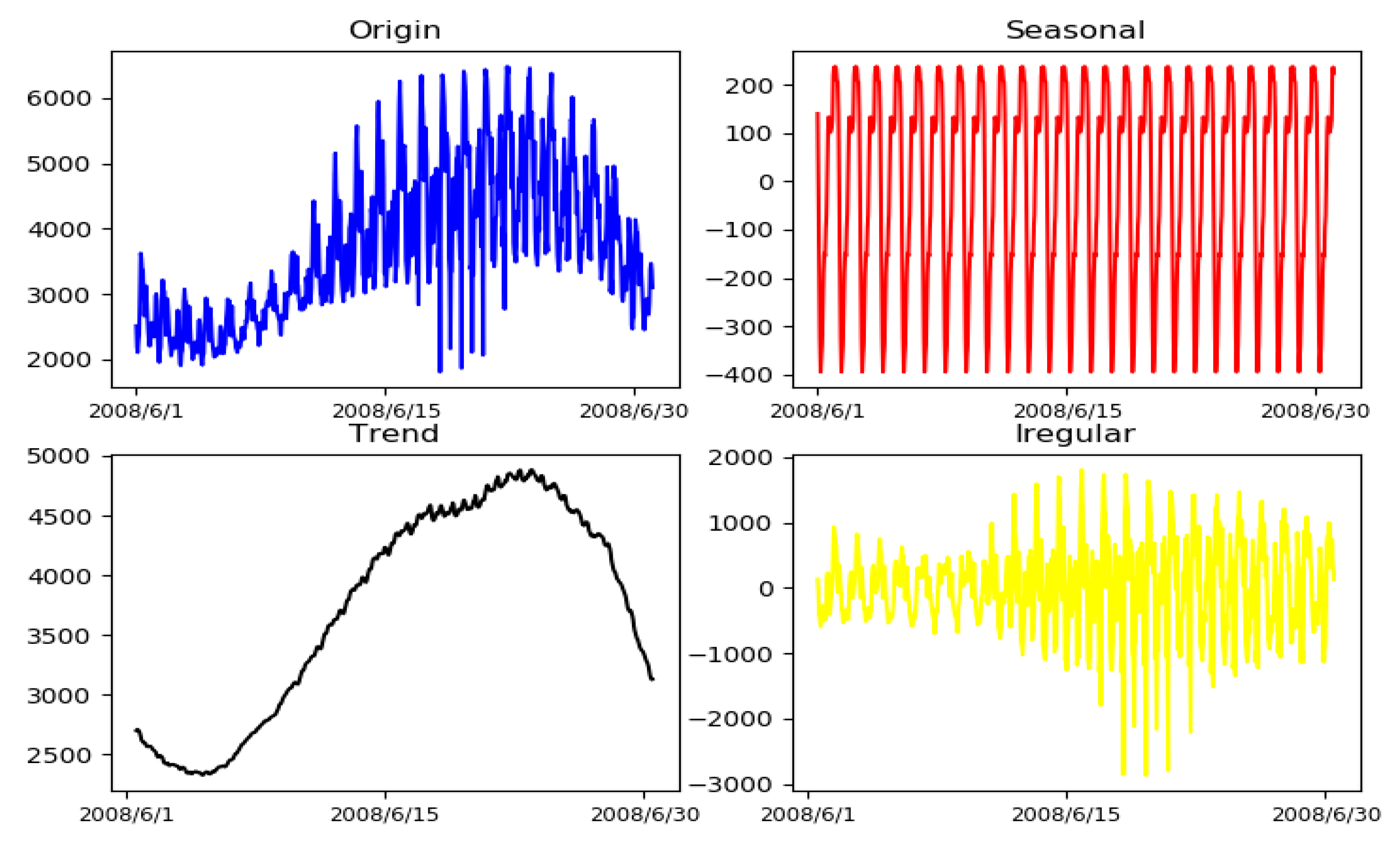
2.2. Seasonal and Trend Adjustment

For time series regression, seasonal and trend adjustment is a process to improve the properties of the parameter estimates. Seasonal and trend adjustment often helps better understand time series data. For instance, if electric consumption in June is up 20% from May. By decomposed data, it is easier to find out that rising of electric consumption is mainly caused by seasonal effects associated with weather. Therefore, to gain better power forecasting results, it is important to decompose original electric series first.

Denote $Y_t$ as the actual time series value at period t. The time series seasonal and trend adjustment approach decomposes $Y_t$ into three components: A trend component, a seasonal component, and an irregular component. These three components are combined by an additive or a multiplicative model.

An additive decomposition model is defined as:

$$Y_t=Tren{d}_t+Seasona{l}_t+Irregula{r}_t$$

(1)

And a multiplicative decomposition model is defined as:

$$Y_t=Tren{d}_t\times Seasona{l}_t\times Irregula{r}_t$$

(2)

where $Tren{d}_{t }$ = trend value at time period t$; Seasona{l}_t$ = seasonal index at time period t$; Irregula{r}_t$ = irregular index at time period t.

The multiplicative model is suitable for situations where the seasonal fluctuations change over time. When the seasonal fluctuations do not depend on the level of the time series, it is good to use the additive decomposition model.

Other than above two basic decomposition models, the decomposition model can also be defined as:

$$Y_t=Seasona{l}_t+Trend and Irregula{r}_t$$

(3)

when the seasonal component is changing slowly, we can use model (3) to decompose time series. As a result, the non-seasonal forecasting model can be applied to a combination of trend and irregular components. A similar model can be applied to the multiplicative model as well:

$$Y_t=Seasona{l}_t\times Trend and Irregula{r}_t$$

(4)

In this paper, we used the electric load data from GEFCOM2012 [29] to explain the implementation of the hybrid model. Figure 2 shows the seasonal and trend decomposition process for load demand of zone 1. As Figure 2 shows, the electric load pattern shows randomness. However, it can be seen from the analysis of weekly electricity seasonal decomposition results that the seasonal and trend components have less volatility, which makes it easier to predict future seasonal and trend components. Although regularity of the irregular component is not obvious, the magnitude of the irregular component is much smaller than the magnitude of the original electric load series. As a result, the prediction accuracy of the method applying the prediction model on three sub-components separately can be better than that of the method making a prediction on original electric load series directly.

2.3. Attention-Based Models

The attention-based model proposed in this paper is depicted in Figure 3. Basically, the model consists of three components: An encoder network, a multi-head attention model, and a decoder network. Composed of a deep recurrent neural network, the encoder network reads the sequence of electric load series x and calculates a sequence of encoded features $h^{enc}=\left(h_1^{enc},\dots ,h_T^{enc}\right)$. The multi-head attention mechanism generalizes the output of the encoder according to the current state of the decoder to calculate a context vector $c_u$, as depicted in Section 2.4. The decoder network is comprised of a deep recurrent neural network modeling an output distribution over the sequence of previous prediction.

2.4. Encoder with Multi-Head Attention

For a regular encoder–decoder architecture, an encoder transforms the input signal $X=\left\{x_1,x_2,\dots ,x_T\right\}$ into a representation vector $V=\left\{v_1,v_2,\dots ,v_T\right\}$.

$$\left[\begin{array}{c}{v}_t\\ h_t\end{array}\right]=\varphi \left(x_t\right)$$

(5)

where $h_t\in R^n$ is a hidden state at time t. The framework of an encoder varies in different applications. For instance, a recurrent neural network (RNN) is widely chosen as an encoder in machine translation. In the field of image caption, it is natural to use a convolutional neural network (CNN) as the encoder. While applied to load forecasting, LSTM is the most appropriate algorithm, since LSTM can efficiently mitigate the problem caused by the gradient vanishing of RNN and transfers the state of hidden layers through forget gate, input gate, and output gate.

By encoding the necessary information in a sequence, bidirectional long short-term memory (BiLSTM) brings outstanding performance [30]. Therefore, BiLSTM was selected as an encoder to take the temporal relation of electric load into account. BiLSTM splits a normal LSTM neuron into two directions, one is the forward states, and the other is backward states. In addition, the output of these two states is not related. By using two directions, the future and past sequence information of the current electric load can be applied.

Figure 4 is the flow diagram of BiLSTM. First, the forward LSTM reads the forward input sequence (from $x_1$ to $x_T$) and computes the forward hidden states ($\overrightarrow{h_1},\dots ,\overrightarrow{h_T}$). At the same time, the backward LSTM reads the sequence in the opposite direction to obtain a series of backward hidden states ($\overleftarrow{h_1},\dots ,\overleftarrow{h_T}$). By concatenating the forward hidden state $\overrightarrow{h_1}$ and the backward hidden state $\overleftarrow{h_1}$, an annotation $v_t$ for each $x_t$ is obtained. As a result, the annotation $v_t$ has the knowledge of both the preceding and the following electric loads.

Multi-headed attention (MHA) was first applied in machine translation [31]. Now, we explore this work in load forecasting. In MHA architecture, each head can produce a different distribution of attention. Therefore, each head plays a different role in attending the encoder output, which makes it easier for the decoder to retrieve information from the encoder. In detail, the model applies M independent attention heads. Each calculates attention values, ${\beta }_{t,u}^i\in R$, for $1\le i\le M,1\le t\le T$:

$${\beta }_{t,u}^i=u^i\tan \mathrm{h}\left(W^i{h}_{u-1}^{att}+V^i{h}_t^{enc}\right)$$

(6)

Then, each attention value is converted into a soft attention weight by a softmax operation, which is employed to calculate a summary of encoder features, $c_u^i$:

$$\begin{array}{c}{\alpha }_{t,u}^i=\frac{\exp \left({\beta }_{t,u}^i\right)}{{\sum }_{s=1}^T\exp \left({\beta }_{s,u}^i\right)}\\ c_u^i={\displaystyle {\displaystyle \sum }_{t=1}^T}{\alpha }_{t,u}^i{Z}^i{h}_t^{enc}\end{array}$$

(7)

Finally, the individual summaries are concatenated together to calculate the overall context vector: $c_u=\left[c_u^1;c_u^2;\dots ;c_u^M\right]$.

2.5. Decoder

In the decoder, we combine the weighted summed context vector $c_{t^{\prime }}$ at a future step $t^{\prime }$ with the last output of decoder ${\widehat{y}}_{t^{\prime }-1}^i$. Then, the hidden state of decoder is updated with $d_{t^{\prime }}=f_d\left(d_{t^{\prime }-1},\left[{\widehat{y}}_{t^{\prime }-1}^i;c_{t^{\prime }}\right]\right)$, where $f_d$ represents an LSTM unit used in the decoder.

Eventually, the final prediction can be calculated as below:

$${\widehat{y}}_{t^{\prime }}^i=V_y^T\left(W_y\left[d_T,c_T\right]+b_w\right)+b_v$$

(8)

where $\left[d_T,c_T\right]\in R^{p+m}$ is a concatenation of the decoder hidden state and the context vector.

The parameters $W_y\in R^{p\times \left(p+m\right)}$ and $b_w\in R^p$ map the concatenation to the size of the decoder hidden states. We use a linear function with weights $V_y$ and bias $b_v$ to produce the final prediction output.

3. Experiments and Results

To verify the forecasting accuracy of the proposed STA–AED model, a real-world dataset from the United States was used for validation purposes in this section, and the experiments are described and analyzed elaborately. The comparisons with random forest, gradient boosting decision tree (GBDT), GRU, encoder–decoder, encoder–decoder with multi-head attention, and the proposed STA–AED model are also analyzed in detail.

3.1. Dataset Description

This paper used an electric load dataset from GEFCOM2012 [29], which includes hour loads from 20 zones in the United States. We used load data from 1 January 2007 to 30 June 2008 in this paper. The data sampling interval was one hour. All test data consisted of 13,128 observations. In this study, the load data from 1 January 2007 to 31 May 2008 were used as a training set, and the load data from 1 June 2008 to 20 June 2008, which are the data of the last month in the original dataset, were used as a testing set. As an example, hourly load data in zone 12 and zone 15 from 1 May 2008 to 30 June 2008 are shown in Figure 5.

In the original dataset, there were 20 geographical zones in all. According to analysis in [29], data from zones 2, 3, 4, 8, and zone 10 were not used because of data duplication. Therefore, we only used data from the remaining 15 zones in this paper.

In this paper, we used the additive model to decompose the electric load series, and the decomposing interval was set as weekly. Figure 6 shows a sample of the seasonal and trend decomposition process for load demand of zone 12. It demonstrates that trend and seasonal components can be separated from original load demand data by seasonal and trend decomposition. Both trend and seasonal components exhibit a clear pattern.

3.2. Model Evaluation Indexes

The mean absolute percentage error (MAPE) and the root mean square error (RMSE) were calculated to evaluate forecasting accuracy. The smaller the values of MAPE and RMSE, the better the forecasting accuracy. The error measures are defined as follows:

$$MAPE=\frac{{{\displaystyle \sum }}_{i=1}^N\left|\frac{\left(P_i-A_i\right)}{A_i}\right|}{N}\times 100\%$$

(9)

$$RMSE=\sqrt{\frac{1}{N}{\displaystyle \sum }_{I=1}^N{\left(P_i-A_i\right)}^2}\times 100\%$$

(10)

where N is the forecasting period, and $P_i$ and $A_i$ are the $i_{th}$ predicted and actual values, respectively.

3.3. Method Comparison

To evaluate the effectiveness of the proposed approach in this paper, two traditional machine learning methods and another three deep learning approaches were implemented as counterparts for compassion purpose. The following are simple introductions for these five counterparts:

(1)

Random forest regressor: Random forest regressor is one of the most widely used traditional machine learning methods.

(2)

Gradient boosting decision tree (GBDT): GBDT is one of the commonly used machine learning algorithms. It is very popular in load forecasting because of its excellent automatic feature combination ability and efficient operation.

(3)

Gated recurrent units (GRUs): GRUs are a widely used variant of the recurrent neural network (RNN). GRUs are similar to long short-term memory (LSTM) but with fewer parameters than LSTM.

(4)

Encoder–decoder: This approach is based on encoder–decoder architecture without applying the attention mechanism.

(5)

Encoder–decoder with multi-head attention: The only difference with the method proposed in this paper is that the input data are not processed by the seasonal and trend decomposing technique.

To make a fair comparison, we also applied seasonal and trend adjustment on all counterpart methods. We use the prefix “STA”, which stands for seasonal and trend adjustment—for instance, STA–GBDT.

3.4. The Detailed Exprimental Setting

In this paper, the proposed method was used to predict the load of the next 24 h, and the past 3 × 24 h load data were used as the input variable of the model. The learning rate was 0.001 and the batch size for both the encoder and decoder were 128. The hidden neuron of the LSTM module was set as 128. The rectified linear unit (ReLU) function was used as the active function. The Adam Optimizer was used to optimize the parameters of the model by performing mini-batch stochastic gradient descent (SGD). The model was trained by the objective function of the standard mean square error. We implemented seasonal and trend decomposition in statsmodels and deep learning method in the PyTorch framework, and ran all the experiments with one GTX 1080Ti GPU.

3.5. Experimental Results and Analysis

The proposed method was used to forecast the load data from 1 June 2008 to 30 June 2008. The prediction results of zone 7 are depicted in Figure 7. As Figure 7 shows, the prediction values are very close to the actual values, except the peak and bottom part.

Table 1. MAPE values for all 15 zones. The lowest value is shown in bold.

Zone Number	Random Forest Regressor	STA–Random Forest Regressor	GBDT	STA–GBDT	GRU	STA–GRU	Encoder–Decoder	STA–Encoder–Decoder	Encoder–Decoder Attention	STA–AED
1	13.77%	16.24%	13.16%	15.71%	13.09%	6.12%	8.59%	6.54%	3.80%	2.70%
5	18.70%	21.21%	18.19%	16.62%	10.87%	8.99%	10.25%	7.65%	5.07%	4.16%
6	10.39%	12.16%	9.87%	10.10%	9.55%	4.05%	7.59%	4.25%	3.26%	2.18%
7	10.09%	11.95%	9.58%	10.02%	8.78%	4.12%	6.50%	3.80%	2.31%	2.26%
9	10.39%	13.68%	15.63%	18.45%	10.15%	8.52%	9.58%	5.66%	9.97%	2.02%
11	13.16%	17.36%	12.37%	14.31%	11.13%	5.77%	8.65%	5.08%	2.79%	2.91%
12	13.94%	17.19%	13.83%	17.93%	11.06%	6.79%	9.32%	6.37%	4.58%	2.25%
13	12.84%	14.06%	11.77%	12.53%	10.41%	7.25%	8.59%	6.12%	5.87%	5.26%
14	15.74%	21.56%	15.85%	19.82%	13.24%	7.86%	10.57%	7.67%	7.33%	6.11%
15	10.87%	17.58%	9.99%	17.11%	9.05%	6.53%	7.56%	6.30%	6.34%	4.73%
16	14.75%	19.66%	14.03%	17.89%	11.79%	7.13%	8.23%	6.42%	5.23%	4.95%
17	10.24%	14.08%	9.77%	12.51%	9.02%	5.22%	6.34%	4.89%	3.64%	2.73%
18	13.53%	16.87%	12.79%	14.75%	10.15%	6.53%	7.21%	5.87%	4.30%	3.90%
19	15.01%	18.22%	15.14%	17.21%	12.37%	7.46%	8.34%	7.12%	6.91%	4.98%
20	10.35%	13.01%	9.67%	11.41%	9.02%	5.33%	7.25%	5.10%	4.27%	3.78%

and

Table 2. RMSE values for all 15 zones. The lowest value is shown in bold.

Zone Number	Random Forest Regressor	STA–Random Forest Regressor	GBDT	STA–GBDT	GRU	STA–GRU	Encoder–Decoder	STA–Encoder–Decoder	Encoder–Decoder Attention	STA–AED
1	2663.64	4721.40	2550.32	4473.39	1912.17	1312.31	1355.67	925.86	881.57	731.64
5	1327.91	2121.71	1306.42	1870.86	1182.13	792.49	756.32	535.86	489.90	382.97
6	19317.86	30628.96	18760.28	26958.93	13131.39	9216.30	12115.67	8642.18	6868.42	4854.46
7	19411.65	31197.98	18858.14	27094.56	12446.93	9704.31	8752.35	7105.42	6170.82	5419.37
9	7289.98	9179.87	9907.69	18006.75	8518.75	7026.93	7568.50	6859.89	7175.57	5476.51
11	14860.07	31699.12	14007.46	27006.26	12828.20	8415.57	8531.56	6523.21	3749.97	4625.02
12	19785.30	47365.13	19417.93	41700.66	17923.31	12499.21	14321.34	8953.23	6868.09	5466.82
13	2589.48	3498.78	2409.35	3121.04	1894.69	1680.42	1859.23	1675.42	1451.41	1412.30
14	3409.58	7096.82	3508.16	6586.08	3367.25	2333.92	2532.56	2035.43	1896.70	1817.25
15	7191.28	15457.41	6735.61	14092.31	5316.52	5253.35	6231.34	5071.21	4466.80	4462.52
16	4564.60	8572.97	4292.14	7498.77	3942.94	2656.92	3587.23	2875.32	2023.26	1813.00
17	3753.61	7179.55	3628.80	6493.66	3035.14	2318.65	2653.54	2012.67	1546.58	1366.90
18	30252.61	53231.76	28873.02	46827.62	21374.29	17821.83	19876.34	15321.43	12758.16	12275.82
19	12488.28	22224.10	12547.69	20381.70	8957.18	7885.67	8531.47	7031.15	6533.16	6056.17
20	9845.51	16640.13	9173.17	15172.12	5937.26	5925.59	8765.21	5768.77	5407.09	4651.63

summarize the experimental results for all 15 zones, in terms of MAPE and RMSE. Table 1 and Table 2 show that the MAPE and RMSE of the random forest regressor are the largest in 12 out of 15 zones. The performance of GBDT is slightly better than the random Forest regressor. It is obvious that the performance of the deep neural networks is much superior than GBDT and the random forest regressor. The results of the GRU modules are a little better than GBDT and the random forest regressor, and the results of the encoder–decoder architecture are better than GRU. The prediction accuracy of two attention-based modules are much better than the rest of the modules. From Table 1 and Table 2, we observe that in 14 out of 15 zones, the solution generated by the proposed model is associated with the lowest RMSE and MAPE values. In fact, in 13 out of 15 zones, MAPE obtained by the STA–AED model is less than 5%, which shows model superiority in the field of short-term load forecasting. When applying seasonal and trend adjustment on both GBDT and the random forest regressor, the prediction accuracy got worse in all 15 experiments—while for all deep learning approaches, the prediction accuracy could be improved in 14 out 15 experiments by applying the seasonal and trend adjustment technique. We think it is because seasonal and trend adjustment takes better effect in deep learning environment. In conclusion, our proposed STA–AED model can make a more accurate forecast by integrating the seasonal and trend decomposing technique and an encoder–decoder network with a multi-head attention mechanism.

Meanwhile, our proposed model is more stable than the other forecasting approaches. Figure 8 and Figure 9 show the comparison results for all 6 approaches in all 15 zones, in terms of MAPE and RMSE, respectively. Figure 8 and Figure 9 show that the curves representing the proposed STA–AED model are approximately the smallest in all zones. Although the encoder–decoder network with multi-head attention shows the best prediction result in zone 11, it is just slightly better than the proposed STA–AED model. To summarize, the proposed STA–AED model achieved good prediction results in all 15 zones, which demonstrates that the proposed STA–AED model can provide better load forecasting ability and can improve the stability of short-term load forecasting.

4. Conclusions

This paper proposes a hybrid deep learning framework for short-term load forecasting. The proposed model is based on the seasonal and trend decomposing technique and the encoder–decoder with a multi-head attention mechanism. The proposed model is validated on a real-word electrical dataset of the United States. The experimental results show that the prediction ability and stability of the proposed STA–AED model are better than that of all the other comparison models, and the best prediction results are obtained in 14 out of 15 zones, which demonstrates the superiority and stability of the proposed model. In the future, applying other attention-based mechanisms on load forecasting can be further investigated.

References

- Yukseltan, E.; Yucekaya, A.; Bilge, A.H. Forecasting electricity demand for Turkey: Modeling periodic variations and demand segregation. Appl. Energy 2017, 193, 287–296. [Google Scholar] [CrossRef]
- Raza, M.Q.; Khosravi, A. A review on artificial intelligence based load demand forecasting techniques for smart grid and buildings. Renew. Sustain. Energy Rev. 2015, 50, 1352–1372. [Google Scholar] [CrossRef]
- Yang, H.; Huang, C.M. A new short-term load forecasting approach using self-organizing fuzzy ARMAX models. IEEE Trans. Power Syst. 1998, 13, 217–225. [Google Scholar] [CrossRef]
- Lee, C.M.; Ko, C.N. Short-term load forecasting using lifting scheme and ARIMA models. Expert Syst. Appl. 2011, 38, 5902–5911. [Google Scholar] [CrossRef]
- Vu, D.H.; Muttaqi, K.M.; Agalgaonkar, A.P.; Bouzerdoum, A. Short-term electricity demand forecasting using autoregressive based time varying model incorporating representative data adjustment. Appl. Energy 2017, 195, 790–801. [Google Scholar] [CrossRef]
- Chen, Y.; Xu, P.; Chu, Y.; Li, W.; Wu, Y.; Ni, L.; Bao, Y.; Wang, K. Short-term electrical load forecasting using the Support Vector Regression (SVR) model to calculate the demand response baseline for office buildings. Appl. Energy 2017, 195, 659–670. [Google Scholar] [CrossRef]
- Avami, A.; Boroushaki, M. Energy Consumption Forecasting of Iran Using Recurrent Neural Networks. Energy Sour. Part B Econ. Plan. Policy 2011, 6, 339–347. [Google Scholar] [CrossRef]
- Lloyd, J.R. GEFCom2012 hierarchical load forecasting: Gradient boosting machines and Gaussian processes. Int. J. Forecast. 2014, 30, 369–374. [Google Scholar] [CrossRef]
- Liu, N.; Tang, Q.; Zhang, J.; Fan, W.; Liu, J. A hybrid forecasting model with parameter optimization for short-term load forecasting of micro-grids. Appl. Energy 2014, 129, 336–345. [Google Scholar] [CrossRef]
- Tripathi, M.M.; Upadhyay, K.G.; Singh, S.N. Short-Term Load Forecasting Using Generalized Regression and Probabilistic Neural Networks in the Electricity Market. Electr. J. 2008, 21, 24–34. [Google Scholar] [CrossRef]
- Guan, C.; Luh, P.B.; Michel, L.D.; Wang, Y.; Friedland, P.B. Very Short-Term Load Forecasting: Wavelet Neural Networks with Data Pre-Filtering. IEEE Trans. Power Syst. 2013, 28, 30–41. [Google Scholar] [CrossRef]
- Shi, H.; Xu, M.; Li, R. Deep Learning for Household Load Forecasting—A Novel Pooling Deep RNN. IEEE Trans. Smart Grid 2017, 9, 5271–5280. [Google Scholar] [CrossRef]
- Hochreiter, S.; Schmidhuber, J. Long Short-Term Memory. Neural Comput. 1997, 9, 1735–1780. [Google Scholar] [CrossRef] [PubMed]
- Gensler, A.; Henze, J.; Sick, B.; Raabe, N. Deep Learning for solar power forecasting—An approach using AutoEncoder and LSTM Neural Networks. In Proceedings of the IEEE International Conference on Systems, Man, and Cybernetics (SMC), Budapest, Hungary, 9–12 October 2016; pp. 002858–002865. [Google Scholar]
- Chen, Z.; Sun, L. Short-Term Electrical Load Forecasting Based on Deep Learning LSTM Networks. Electr. Technol. 2018, 158, 2922–2927. [Google Scholar]
- Lu, K.; Zhao, Y.; Wang, X.; Cheng, Y.; Pang, X.; Sun, W.; Jiang, Z.; Zhang, Y.; Xu, N.; Zhao, X. Short-term electricity load forecasting method based on multilayered self-normalizing GRU network. In Proceedings of the IEEE Conference on Energy Internet and Energy System Integration, Beijing, China, 26–28 November 2017; pp. 1–5. [Google Scholar]
- Zheng, J.; Xu, C.; Zhang, Z.; Li, X. Electric load forecasting in smart grids using Long-Short-Term-Memory based Recurrent Neural Network. In Proceedings of the 2017 51st Annual Conference on Information Sciences and Systems (CISS), Baltimore, MD, USA, 22–24 March 2017. [Google Scholar]
- Wang, Y.; Liu, M.; Bao, Z.; Zhang, S. Short-Term Load Forecasting with Multi-Source Data Using Gated Recurrent Unit Neural Networks. Energies 2018, 11, 1138. [Google Scholar] [CrossRef]
- Park, S.H.; Kim, B.; Kang, C.M.; Chung, C.C.; Choi, J.W. Sequence-to-Sequence Prediction of Vehicle Trajectory via LSTM Encoder-Decoder Architecture. In Proceedings of the 2018 IEEE Intelligent Vehicles Symposium (IV), Changshu, China, 26–30 June 2018. [Google Scholar]
- Jiang, X.; Xiao, Z.; Zhang, B.; Zhen, X.; Cao, X.; Doermann, D.; Shao, L. Crowd Counting and Density Estimation by Trellis Encoder-Decoder Network. Available online: https://arxiv.org/abs/1903.00853 (accessed on 15 September 2019).
- Fernando, T.; Denman, S.; Sridharan, S.; Fookes, C. Soft + Hardwired Attention: An LSTM Framework for Human Trajectory Prediction and Abnormal Event Detection. Neural Netw. 2017, 108, 466–478. [Google Scholar] [CrossRef]
- Bahdanau, D.; Cho, K.; Bengio, Y. Neural Machine Translation by Jointly Learning to Align and Translate. arXiv 2014, arXiv:1409.0473. [Google Scholar]
- Cheng, W.; Shen, Y.; Zhu, Y.; Huang, L. A Neural Attention Model for Urban Air Quality Inference: Learning the Weights of Monitoring Stations. In Proceedings of the National Conference on Artificial Intelligence, New Orleans, LA, USA, 2–7 February 2018; pp. 2151–2158. [Google Scholar]
- Ma, F.; Chitta, R.; Zhou, J.; You, Q.; Sun, T.; Gao, J. Dipole: Diagnosis Prediction in Healthcare via Attention-based Bidirectional Recurrent Neural Networks. In Proceedings of the 23rd ACM SIGKDD International Conference on Knowledge Discovery and Data Mining, Halifax, NS, Canada, 13–17 August 2017; pp. 1903–1911. [Google Scholar]
- Paparoditis, E.; Sapatinas, T. Short-Term Load Forecasting: The Similar Shape Functional Time Series Predictor. IEEE Trans. Power Syst. 2012, 28, 3818–3825. [Google Scholar] [CrossRef]
- Wu, J.; Wang, J.; Lu, H.; Dong, Y.; Lu, X. Short term load forecasting technique based on the seasonal exponential adjustment method and the regression model. Energy Convers. Manag. 2013, 70, 1–9. [Google Scholar] [CrossRef]
- Wang, J.; Li, L.; Niu, D.; Tan, Z. An annual load forecasting model based on support vector regression with differential evolution algorithm. Appl. Energy 2012, 94, 65–70. [Google Scholar] [CrossRef]
- Ribeiro, M.; Grolinger, K.; ElYamany, H.F.; Higashino, W.A.; Capretz, M.A. Transfer Learning with Seasonal and Trend Adjustment for Cross-Building Energy Forecasting. Energy Build. 2018, 165, 352–363. [Google Scholar] [CrossRef]
- Taieb, S.B.; Hyndman, R.J. A gradient boosting approach to the Kaggle load forecasting competition. Int. J. Forecast. 2014, 30, 382–394. [Google Scholar] [CrossRef]
- Ji, Z.; Xiong, K.; Pang, Y.; Li, X. Video Summarization with Attention-Based Encoder-Decoder Networks. CoRR 2017, abs/1708.09545. [Google Scholar] [CrossRef]
- Vaswani, A.; Shazeer, N.; Parmar, N.; Uszkoreit, J.; Jones, L.; Gomez, A.N.; Kaiser, Ł.; Polosukhin, I. Attention is All You Need. In Proceedings of the Conference on Neural Information Processing Systems, Long Beach, CA, USA, 4–9 December 2017; pp. 5998–6008. [Google Scholar]