Article

Estimation of Impedance and Susceptance Parameters of a 3-Phase Cable System Using PMU Data

1
Electrical Energy Systems Group, Eindhoven University of Technology, 5600 MB Eindhoven, The Netherlands
2
VSL, 2629 JA Delft, The Netherlands
*
Author to whom correspondence should be addressed.
Energies 2019, 12(23), 4573; https://doi.org/10.3390/en12234573
Submission received: 29 September 2019 / Revised: 28 October 2019 / Accepted: 29 October 2019 / Published: 30 November 2019
(This article belongs to the Special Issue 2nd International Colloquium on Smart Grid Metrology (SmaGriMet 2019))

Abstract

:
This paper proposes a new regression-based method to estimate resistance, reactance, and susceptance parameters of a 3-phase cable segment using phasor measurement unit (PMU) data. The novelty of this method is that it gives accurate parameter estimates in the presence of unknown bias errors in the measurements. Bias errors are fixed errors present in the measurement equipment and have been neglected in previous such attempts of estimating parameters of a 3-phase line or cable segment. In power system networks, the sensors used for current and voltage measurements have inherent magnitude and phase errors whose measurements need to be corrected using calibrated correction coefficients. Neglecting or using wrong error correction coefficients causes fixed bias errors in the measured current and voltage signals. Measured current and voltage signals at different time instances are the variables in the regression model used to estimate the cable parameters. Thus, the bias errors in the sensors become fixed errors in the variables. This error in variables leads to inaccuracy in the estimated parameters. To avoid this, the proposed method uses a new regression model using extra parameters which facilitate the modeling of present but unknown bias errors in the measurement system. These added parameters account for the errors present in the non- or wrongly calibrated sensors. Apart from the measurement bias, random measurement errors also contribute to the total uncertainty of the estimated parameters. This paper also presents and compares methods to estimate the total uncertainty in the estimated parameters caused by the bias and random errors present in the measurement system. Results from simulation-based and laboratory experiments are presented to show the efficacy of the proposed method. A discussion about analyzing the obtained results is also presented.

1. Introduction

Accurate estimates of line parameters are useful in improving the performance of power system monitoring and protection applications like accurate relay settings and fault location [1]. Distance relays have reach zone settings based on the known positive sequence impedance of the protected line segment. High accuracy impedance estimates of the protected line would assist in a more accurate setting of the impedance in the distance relay which protects the line. It is known that accurate pre-fault line impedance and knowledge about impedance of loads on the line could be utilized to calculate the location of the faults more precisely [2]. A novel idea of utilizing real-time resistance estimates to monitor the temperature of an overhead line or a cable and facilitate dynamic line rating (DLR) was first mentioned in [3]. It was presented that the relationship between the conductor resistance and temperature could be utilized to estimate the real-time temperature of the conductor. The estimated temperature could then be utilized to access the thermal state and set flexible loading levels of power lines in real-time. For cables, parameters (resistance (R), reactance (X) and susceptance (B)) have been calculated using the available information and assumptions on the physical attributes of the cable segment like length, conductor dimension, ambient soil temperature, and moisture content. However, these methods are static in nature as the used specifications are considered constant for long periods, while the cable resistance could change based on ambient temperature and loading levels. Monitoring of cable temperature in real time and implementation of DLR based on the cable temperature would require more reliable and frequent estimates of the cable parameters (especially resistance).
To facilitate the first step of temperature based DLR (monitoring of cable conductor temperature), this paper proposes a method to estimate the resistance of 3-phase cable system utilizing real-time phasor measurement unit (PMU) measurements. Other parameters like cable reactance and susceptance are also estimated alongside. When compared to the previous methods, the proposed method is suitable for a 3-phase system and gives more accurate results in the presence of errors in the measurement equipment. The proposed method also facilitates a more reliable estimation of the uncertainty in the achieved results.
In the recent past, methods have been presented that utilize PMU data to estimate the overhead-line parameters [4,5,6,7,8]. These methods estimate line parameters utilizing voltage and current phasors at both ends of the line segment and could give frequent parameter estimates. The authors in [5] presented an ordinary least squares (OLS)-based regression method to estimate the impedance parameters of an overhead transmission line. The effect of random errors in the phasor measurements were analyzed. However, the effect of bias error in the measurements was not considered. The bias error comes from the magnitude and phase errors in the measurement sensors. For medium voltage (MV) and high voltage (HV) networks, these sensors are current and voltage transformers (CTs and VTs, respectively) which transform the current and voltage signals into low amplitude signals before feeding to the PMUs. As is shown later, the bias errors in the measurements contribute to the total error in the parameter estimates. A novel method for estimating the parameters of an overhead transmission line was described in [6], where the bias errors are accounted for while estimating the parameters. However, to estimate the correct bias correction coefficients, the authors use an assumption that the resistance varies linearly over a short period relative to the time constant of the conductor. Moreover, the estimation algorithm is developed and tested only for single phase lines. Three-phase lines have mutual coupling elements and estimating the parameters has challenges in terms of modeling and signal excitation requirements. Hence, it was noted in [7] that the application of such an algorithm for 3-phase lines would require more complex models. Also, no tests were done to demonstrate the performance of the method for actual measurements. A three-phase parameter estimation problem using a robust parameter estimation is discussed in [8]. The paper also describes the importance of power system operating conditions characterized by characteristics like correlation, dependence and level of unbalance between the three-phase voltage and current signals on the overall uncertainty of the estimates. A field test of a fully transposed overhead HV transmission line was done to demonstrate the algorithm. However, for their field test, the bias correction coefficients for both ends of the VTs were already known. Thus, none of the previous methods are suitable to estimate parameters of a 3-phase cable system in the presence of both random and bias errors in the measurement chain.
In previous works [5,7], the metrics for the evaluation of the results were based on the knowledge of the actual parameter values. However, in the real application cases, reference values are either not available or are not reliable enough to the desired level. This makes this type of validation process less suitable for application using real-field data, since the reference parameters might have changed depending on the ambient environmental and power system operating conditions. The authors in [8] also specified that there was a discrepancy between parameters they estimated and the reference value of those. The highest difference observed was of 13% in the estimated resistance. In the absence of a reliable reference, this could not be explained. Hence, it is very important to have a reliable measure of uncertainty associated with the estimated parameters.
This paper presents solutions to both concerns stated above. It presents a method which is capable of providing accurate parameter estimates even in the presence of unknown bias errors in the sensors. It also presents and compares different methods to calculate the total uncertainty associated with the parameter estimates. It is mentioned in [8] that factors like unbalanced loading levels and some independence in the power flow in the 3 phases are the necessary conditions for convergence of the algorithm. The absence of unbalanced and independent power flow could cause the OLS problem to become ill-conditioned. However, the effects of such an ill-conditioned OLS problem on the uncertainty of parameter results was not discussed in detail. This paper also presents a discussion on the condition of the measurement matrices and its effect on the results.
The remainder of the paper is arranged as follows: Section 2 discusses the core of the previous line parameter estimation methods, and their drawbacks are discussed. Section 3 presents the new parameter estimation algorithm. Section 4 presents various methods to calculate the uncertainty of the estimated parameters. Section 5 presents the results from the simulation and laboratory tests and evaluates the methods presented for calculation of the uncertainty in the estimated parameters. Discussion about the general guidelines for applying the proposed method is presented in Section 6, and conclusions are drawn in Section 7.

2. Existing Parameter Estimation Methods and Drawbacks

To estimate the parameters of a 3-phase line-segment, two different methods are presented in [5,8]. However, they use the same regression model with different objective functions. A robust objective function was chosen in [8] to get better estimates in the presence of outliers in the measurements. In this paper, both the previous methods are considered to give similar results in the absence of outliers. Hence, both are treated as the same and referred to as the existing method. Results obtained by OLS-based objective function as used in [5] are used for comparison with the proposed method. This section presents and discusses the drawbacks of the regression model used in the existing method.
A 3-phase cable segment is represented by a nominal Pi model. Based on the nominal Pi model shown in Figure 1, relationships between the measured current and voltage at the two ends can be described using Equations (1) and (2).
I a b c S I a b c R = B a b c 2 V a b c S + V a b c R ,
V a b c S V a b c R = Z a b c B a b c 2 V a b c R + I a b c R ,
where Z a b c and B a b c are 3 × 3 matrices of unknown cable parameters with self components as diagonal elements and mutual components as off-diagonal elements. Superscript S/R denotes the sending and receiving end of the cable, and subscripts ABC denote the 3-phases system. Using phasors given by PMUs, voltage and current signals are represented as complex numbers in Cartesian coordinates. Equations (1) and (2) are separated into real and imaginary terms, giving a set of 12 equations. These equations are then solved in linear least-squares sense to estimate the unknown R a b c , X a b c , and B a b c parameters. The set of linear equations with p parameters can be written as:
y i = h 1 i θ 1 + h 2 i θ 2 + . . . + h p i θ p + ϵ i ,
where, according to Equations (1) and (2), y i is made up of real or imaginary parts of Δ I A B C or Δ V A B C , h i j is real or imaginary I A B C or V A B C , and θ j are the cable parameters to be estimated. ϵ i is the error term calculated as the difference between the measured quantity and the result of the linear equation formed by parameters and independent variables. For p parameters and n sets of observations, the whole system of linear equations is represented in matrix form as:
Y [ 12 n × 1 ] = H [ 12 n × p ] θ [ p × 1 ] + E [ 12 n × 1 ] ,
where Y is the measurement vector and θ is the parameters vector. H is the relation matrix formed of variables which are real or imaginary components of the measured voltage and current phasors.
The estimates for parameter θ are given by the equation:
θ = c o v a r i a n c e ( Y , H ) v a r i a n c e ( H ) .
In matrix form, the analytical solution could be found out by solving the OLS problem m i n θ | | Y H θ | | 2 . The solution is given as:
θ = ( H T H ) 1 H T Y .
The analysis of the estimated parameters and residuals is an important as well as challenging part of validation of the results. Given that the system being measured is modeled correctly using Equation (3), the parameters obtained using OLS-based regression are true and unbiased only when the residuals adhere to properties:
(a)
Zero mean error: Residuals have a distribution with zero mean such that E [ ϵ i ] = 0 ;
(b)
No heteroscedasticity: The residuals have a constant variance. Each residual ϵ i has the same finite variance σ 2 ;
(c)
Independent variables: There is no correlation between the residuals and the independent variable, E [ ϵ i | h j 1 , h j 1 , . . . , h j n ] = 0 ;
(d)
Normality: The error vector is normally distributed.
Assumptions ad can be summarized in matrix notation as:
ϵ = N ( 0 , σ 2 I ) .
In field measurements, each of these assumptions might not hold true. Apart from the random measurement errors, field CTs and VTs have a steady bias error in their measurement due to the inherent magnitude and phase errors of different magnitudes. As shown in Equation (3), elements of the matrix H and vector Y are real and imaginary parts of measured current and voltage phasors. The presence of any magnitude and phase errors in the measurement chain would cause a fixed bias error in those elements. Use of the same regression model as in the existing method will result in residuals which will not have a normal distribution. The expected value of residuals might also be non-zero. This indicates a mismatch between the system model used in the regression model and the measurements acquired from the system. Thus, the estimated model parameters will differ from the actual parameters. In such cases of measurements with bias errors, the calculated uncertainty of the parameters would be wrong. This is because the OLS problem formulation assumes that all of the errors are present in the vector Y and have a normal distribution. In the current case of the OLS problem, the variables ( h i j ) are also made up of measured quantities, like current and voltage phasors. These variables, apart from having random noise errors, also have fixed bias errors which do not have a normal distribution. Thus, the existing method does not address the effect of bias errors on the quality of the parameter estimates.
Section 3 presents the proposed method, which gives more accurate results in the presence of bias and random errors in the measured variables. After that, Section 4 presents different methods to estimate the uncertainty in the estimated results in the presence of bias and random errors in the variables.

3. Proposed Method

The proposed method utilizes a more suitable model of the measurement system. While estimating line parameters, it considers the presence of possible errors in the available correction coefficients for magnitude and phase errors in the CTs and VTs. The use of erroneous correction coefficients to correct the CT and VT measurements would lead to systematic bias errors in the measure current and voltage signals. To avoid such conditions, extra parameters in the linear regression model were added which account for the bias errors in the current and voltage measurements.
It can be shown that for a sinusoidal signal of the form V = | M | e j ϕ , the measured signal V m with a magnitude error of γ % and phase error of δ ϕ can be written as: V m = V ( 1 + γ ) e j δ ϕ . These bias errors in the measurements are considered to be constant for the duration of one window length of sampled data. The correction coefficients to correct the bias errors can be represented as e ± j δ ϕ 1 + γ . In Cartesian coordinates, this is represented in the form a ± j b , where a is the real part given by c o s ( ± j δ ϕ ) 1 + γ and b being the imaginary part given by s i n ( ± j δ ϕ ) 1 + γ . Using the correction coefficients at both ends, Equations (1) and (2) for a 3-phase system are rewritten in the following form:
C i S I S C i R I R = B 2 C v S V S + C v R V R ,
C v S V S C v R V R = Z B 2 C v R V R + C i R I R ,
where C i S , C i R , C v S and C v R are the complex three-phase correction coefficients for the magnitude and phase errors of CTs and VTs at both ends of the cable.
Equations (8) and (9) are the difference equations of measured voltage and current phasors. These equations can be rewritten using a new set of Adjusted Correction Coefficients (ACCs):
I S K 1 I R = B 2 K 2 V S + K 3 V R ,
V S K 4 V R = Z K 4 B 2 V R + K 5 I R ,
where:
K 1 = C i R C i S , K 2 = C v s C i S , K 3 = C v R C i S , K 4 = C v R C v S a n d K 5 = C i R C v S
are the ACCs.
The new Equations (10) and (11) are representations of Equations (8) and (9) in a manner that allows us to treat the measurements at one end of the line (the sending end in this case) as bias-error-free. The measurements of the receiving ends are corrected using the ACCs. The number of unknown parameters is still large. The parameter B cannot be estimated along with unknown correction coefficients K 2 and K 3 . If the product of K 4 and B 2 is taken as another coefficient K 6 , then Z cannot be estimated along with K 5 and K 6 . A sensitivity analysis was performed to identify the most prominent correction coefficients. The parameter estimates are more sensitive to the prominent correction coefficients.
For this analysis, a 10 km long MV cable (20 kV) was simulated. The maximum magnitude and phase error in CTs and VTs was limited to 1% in magnitude and 1 in phase. Hence, the CT and VT magnitude errors were varied as per a random uniform distribution in the range between 0% and 1%. Similarly the phase angle errors of the CTs and VTs were varied between 0 anf 1 . The coefficients K 1 K 5 were calculated based on these magnitudes and phase errors and were substituted in Equations (10) and (11) to calculate the deviation in B, Z parameters. The results are presented in Figure 2 and Figure 3. For the simulated system, it was observed that the error in B varied within 1 % due to coefficients K 2 and K 3 individually. At the same time, the error in B is highly sensitive to K 1 . A similar analysis showed that the R and X are sensitive to K 4 .and It was observed that the R and X estimates were little affected by the errors in K 5 and K 6 . Hence, only ACCs K 1 and K 4 were used into the system of linear equations, and B 2 was used instead of K 4 × B 2 .
I S = K 1 I R + B 2 V S + V R
V S = K 4 V R + Z B 2 V R + I R
Equations (12) and (13) represent the updated model utilized by the proposed method to estimate the cable parameters while minimizing the effect of inherent bias in the measured current and voltage signals. These equations can be written as two separate equations for real and imaginary parts. This was done for all the three phases resulting in twelve equations. Now, the parameter estimation process was divided in two parts. All the measured data were arranged according to the six equations from Equation (12), forming an overdetermined system of linear equations. Parameters K 1 and B for all phases were estimated using the analytical solution given by Equation (6). The estimated B parameters were substituted in Equation (13) to estimate resistance (R) and reactance (X) parameters.
After estimation of the parameters, total uncertainty in the estimated values was quantified by confidence interval (CI) associated with each parameter. The next section presents the methods to estimate total uncertainty in the parameter estimates caused by random and bias errors in the measurements of the variables.

4. Estimation of Uncertainty

The accuracy of a parameter estimate is a qualitative characteristic which is made up of components trueness and precision. Quantitative estimates of trueness and precision are given by expected bias and standard deviation, respectively [9]. The guide to the expression of uncertainty in measurement (GUM) specifies ways of evaluating the uncertainty of a measurement. Type A uncertainty evaluation is derived by statistical methods on a series of observations whereas Type B evaluation is based on the specifications given by the equipment manufacturers or calibration reports [10]. However, the system model used to estimate the cable parameters falls under the category of the multivariate multistage measurement model described in GUM [11]. The model specifies the manner in which the parameters are estimated using various input quantities. The standard deviation of OLS parameters is given by the diagonal vector of the covariance of the parameters. This falls under the type A uncertainty evaluation. However, it can be shown that this estimate of uncertainty could be misleading in cases where the residuals do not adhere to the assumptions summarized by Equation (7). This could be caused by an inaccurate measurement model or some bias errors in the measured variables leading to a systematic bias in the parameter estimates. Hence, to get a more accurate representation of uncertainty in the solution of the OLS problem, estimating the component of systematic bias is also important. Hence, combining the bias and standard deviation error would give us the total uncertainty associated with the estimated parameters.
The fixed bias error component in the parameters was evaluated using the knowledge of the bias errors present in each of the equipment. Measurement bias errors of each individual piece of equipment could be evaluated based on the specifications given by the equipment manufacturers. As per GUM, this is categorized as Type B evaluation of uncertainty. The error in parameter estimates due to the bias in the variables can be minimized by the use of correction coefficients if available. Possible errors in the correction coefficients were modeled in the system model using the ACCs K 1 - K 5 . However, in the formulation of the proposed method, correction coefficients K 2 , K 3 K 5 were ignored and assumed to be 1. The product of K 4 and B 2 was considered to be B 2 . The error in the estimated parameters caused by these assumptions was calculated using Monte Carlo-based simulations.
The combined uncertainty of the parameters estimates constitutes the uncertainty caused due to random errors in the measurements and the bias due to the assumptions made on the correction coefficients K 2 , K 3 , K 5 , and K 6 . Separate uncertainties for both random and bias errors were estimated and combined to get a combined CI. Section 4.1, Section 4.2 and Section 4.3 present the three methods evaluated to estimate the uncertainty in the parameters due to random errors in PMU estimates. Estimation of the bias in parameter estimates caused by the bias errors present in the variables is shown in Section 4.4.
It was shown in [12] that for a sinusoidal current or voltage signal X sampled consistent with the Nyquist rate and containing white noise, the expected error in computed phasor ( E [ X ˜ ] ) by a full cycle discrete Fourier transform (DFT) is zero. Hence, the CTs and VTs are a source of fixed bias errors where as the PMUs are the source of random errors in the voltage and current variables.

4.1. Effect of Random Errors: Standard Deviation-Based Uncertainty (Method 1)

Given that the assumptions a d hold true, the covariance matrix of the parameter estimates is given by [13]:
c o v ( θ ) = ( H T H ) 1 σ 2 ,
where σ 2 is the unbiased estimate of the variance of the residuals. The standard deviations in the parameters are calculated by taking the square root of the diagonal elements of the covariance matrix. A coverage factor of 3 was multiplied to get the expanded standard deviation ( α ).
α = 3 × d i a g ( c o v ( θ ) )
Method 1 gives the deviation in parameters caused by random noise in the measurements based on the assumed properties of the OLS system. The system assumes that the errors are in the Y vector only. Section 4.2 and Section 4.3 present two methods which calculate the sensitivity of the OLS solutions due to the random errors in the variables of the H matrix and Y vector.

4.2. Effect of Random Errors: Norm-Wise Boundary of Uncertainty (Method 2)

Due to the presence of random errors, the relationship matrix H and the vector Y are perturbed from their true values. Hence, for given H R ( m n ) and H + Δ H , The OLS problem:
m i n θ | | Y H θ | | 2 , r = Y H θ
in the presence of errors in measurements is transformed into:
m i n θ 1 | | ( Y + Δ Y ) ( H + Δ H ) θ 1 | | 2 , s = Y + Δ Y ( H + Δ H ) θ 1 ,
where s and r are the residuals of the OLS solution with and without the errors in variables. H + Δ H and Y + Δ Y are made up of measured variables with errors and are renamed H m and Y m , respectively. Backward error ( Δ H ) is defined as the error in measured variables used in the OLS problem. The presence of backward error in the variables gives rise to the error in the parameter estimates which is called the forward error ( θ θ 1 ) . Sensitivity of the OLS solution due to errors in variables was investigated in [14,15]. Both component-wise and norm-wise bounds of the forward error could be derived.
Considering the OLS problem shown in Equation (17), Method 2 gives the uncertainty α as the ratio of the euclidean norm of the expected maximum deviation and the estimated parameter vectors. It is shown in [14] that for a perturbation error η and σ 1 and σ n as the biggest and smallest eigenvalues of the matrix H m , if:
η = m a x | | Δ H | | 2 | | H m | | 2 , | | Δ Y | | 2 | | Y m | | 2 < σ n σ 1
and
s i n ( ϕ ) = s | | Y m | | 2 1
are satisfied, then the ratio of norms of the maximum deviation and estimated parameter vectors are given by:
α : = | | θ 1 θ | | 2 | | θ 1 | | 2 η 2 κ c o s ( ϕ ) + t a n ( ϕ ) κ 2 ,
where κ is the condition number of matrix H m . For a given rectangular matrix H, the condition number is defined as:
κ ( H ) = | | H | | 2 | | H + | | 2 ,
where H + is the pseudo-inverse of the matrix H and | | H | | 2 denotes the Frobenius norm of the matrix. Thus, α is the norm-wise boundary of maximum uncertainty caused by the random errors in measurement. For small values of residuals, the maximum uncertainty is twice the condition number of the matrix H m .

4.3. Effect of Random Errors: Component-Wise Boundary of Uncertainty (Method 3)

Method 2 presented the norm-wise boundary of uncertainty in parameter estimates. Method 3 calculates the component-wise boundary for the OLS problem shown by Equation (17). Let E and f be an arbitrary matrix and vector such that:
| Δ H | η E   and   | Δ Y | η f .
The absolute values and inequalities between the matrices and vectors are held component-wise. However, the measured matrix H m has different rows made up of different measurements of different scales, and the total backward error was computed for each row rather than for each component. For e = [ 1 , 1 , . . . 1 ] T , the matrix E and vector f can be formulated as:
E = | H m | e e T   and   f = | | Y | | 1 e .
By doing so, the errors in the ith row of H m are measured as the L1 norm of that row.
Using Equations (16) and (17), and the assumptions binding Δ H and E, it was shown in [15] that the maximum deviation ( α ) in each element of the solution of the OLS problem can be calculated as:
α : = | θ 1 θ | η ( | H m + | ( f + E | θ 1 + | ( H m T H m ) 1 | E T | s | ) ,
where | θ 1 θ | is the maximum deviation given for each individual parameters caused by random errors in measurement.
Section 4.1, Section 4.2 and Section 4.3 presented methods to calculate the deviation in parameter estimates caused by the random errors in the variables. Section 4.4 presents the method to calculate the deviation caused due to the bias in the measured variables.

4.4. Effect of Bias Errors

Although the new proposed method includes the most sensitive ACCs K 1 and K 4 to model the bias errors in the measurements, other coefficients K 2 , K 3 , and K 5 were for the sake of simplicity ignored and hence assumed to be 1. The factor of K 4 × B 2 was kept as B 2 . This would cause deviations in the parameters estimates. This subsection presents a Monte Carlo-based method to estimate the deviation due to the error in the measurement model caused by the assumptions made on of K 2 , K 3 , K 5 , and K 6 correction coefficients.
Equations (10) and (11) were expanded, and the components were written in the complex form. The real and imaginary parts of the equation were separated as done earlier. The magnitude and phase errors were varied in the range of ± 50 % from their last calibrated values. Matrix H i and vector Y i were evaluated for all possible values of coefficients K 2 , K 3 , and K 5 . For each set of H i and Y i , parameters θ i are calculated. The maximum deviation ( β ) in the parameters due to bias errors in the variables is quantified by:
β m a x ( | | θ i θ 1 | | 2 ) | | θ 1 | | 2 ,
for the norm-based analysis and:
β m a x ( | θ i θ 1 | ) | θ 1 | ,
for the component based analysis.
Section 4.1, Section 4.2, Section 4.3 and Section 4.4 presented methods to calculate uncertainties due to random and bias errors in the measurements. The total uncertainty for the parameter estimates was calculated combining the uncertainties due to random and bias errors in the measured variables. The total uncertainty, denoted by a CI in the parameters, is given by:
C I α 2 + β 2 .
Section 3 and Section 4 presented the proposed method to estimate the cable parameters accurately in the presence of random and bias errors in the measurement system and then to calculate the uncertainty associated with the estimation results. The complete process is summarized using a flowchart presented in Figure 4. Model initialization is done at the beginning to select the prominent parameters of the regression model. After initialization, the method can be run in loop to give continuous estimates of the parameters. Section 5 presents the results obtained using the proposed method along with comparisons with the existing method.

5. Results and Comparison

First, both the existing and the proposed methods were tested using simulation tests. A 20 kV, 10 km cable was simulated. The exact values of the parameters of simulated 3-phase cables were known. The obtained results were evaluated based on the analysis of the residuals of the OLS problem shown in Equation (4). If the residual vector seemed to satisfactorily pass the tests to check the assumptions a d , then the uncertainty of the parameters was calculated considering the presence of random errors and bias errors in modeling caused by exclusion of the correction coefficients K 2 , K 3 and K 5 .
In each of the simulation tests, all the other operating and measurement conditions were kept the same for the purpose of a fair comparison. The number of samples collected, the variance in the power flow process, and the noise levels in the measurement process were kept the same across all the tests. A steady-state linear Kalman filter was used to filter out the PMU measurements to avoid any outliers in the PMU data streams. Since the proposed method filters the data before applying them to the regression model, there are no outliers present in the measurements. The robust estimator used in [8] minimized the influence of outliers on the estimation results presented in [5]. Since the outliers are filtered already using the Kalman filter, the existing method is represented by the results from the OLS-based solution used in [5].
After filtering the phasor estimates, the data are used in the estimation process. To examine the results, the residuals were checked for the assumptions of normality and homoscedasticity. To test normality for large data set, a more visual approach was applied, and a QQ-plot was used to evaluate the normality of the residuals. A QQ-plot displays the quantiles of the data under test versus the expected quantile values of a normal distribution [16]. If the distribution of residual is normal, then the plotted residuals in the QQ-plot appear linear. Visual tests can also be done to check for heteroscedasticity to verify that the variance of the residuals does not vary at different measurement values. The same approach was adopted for the following tests. If residuals did not satisfy the criteria for normality and homoscedasticity, then it was an indication that the measurements did not explain the system modeled by Equations (12) and (13) correctly. Simulation and laboratory tests done to show the results of the proposed method and comparison with the existing method are presented next.

5.1. Measurements with No Errors

Accuracy characteristics of 0.1 class and 1.0 class CTs and VTs were used in this test. The sending end bus had 0.1 class equipment, while the receiving end had the 1.0 class. The CTs and VTs were calibrated, and correction coefficients for fixed magnitude and phase errors were known. Table 1 shows the results using the existing method when no random errors were present in the simulated measurement system. The bias errors in the measurements of all the CTs and VTs were corrected. Without any errors, the system of equations used in the existing method and the proposed method are the same, and hence, the estimated parameters were also the same. Since no other errors were modeled, the only source of uncertainty was the numerical resolution of the simulation and processing software. The CIs for each parameter were very small and were lower than 0.01 parts per million (PPM). Actual errors calculated using the reference values of the parameters were also very small and are presented in Table 1.
Table 1 established that the existing method gives accurate parameter estimates in the absence of errors in the measurements. When there are no errors, the equation models used by the proposed method are the same as those in the old method and give the same parameter results and confidence intervals. For the next subsection, random errors were added to the phasor estimates of the PMUs.

5.2. Measurements with Only Random Noise Error

Based on the error specifications given by a commercial PMU manufacturer [17], the random noise errors in PMU phasor estimates were taken to be ± 0 . 02 % and ± 0 . 03 % in voltage and current magnitude, respectively, and ± 0 . 01 in phase angles for both voltage and current. The given errors are the maximum uncertainty expected in the magnitude and phase angles of the estimated phasors. The errors are uniformly distributed with a standard deviation of specified error divided by 3 . The existing and the proposed methods were applied to the filtered PMU data. The number of distinct samples for each measurement was the same. The analysis for results obtained is presented below.
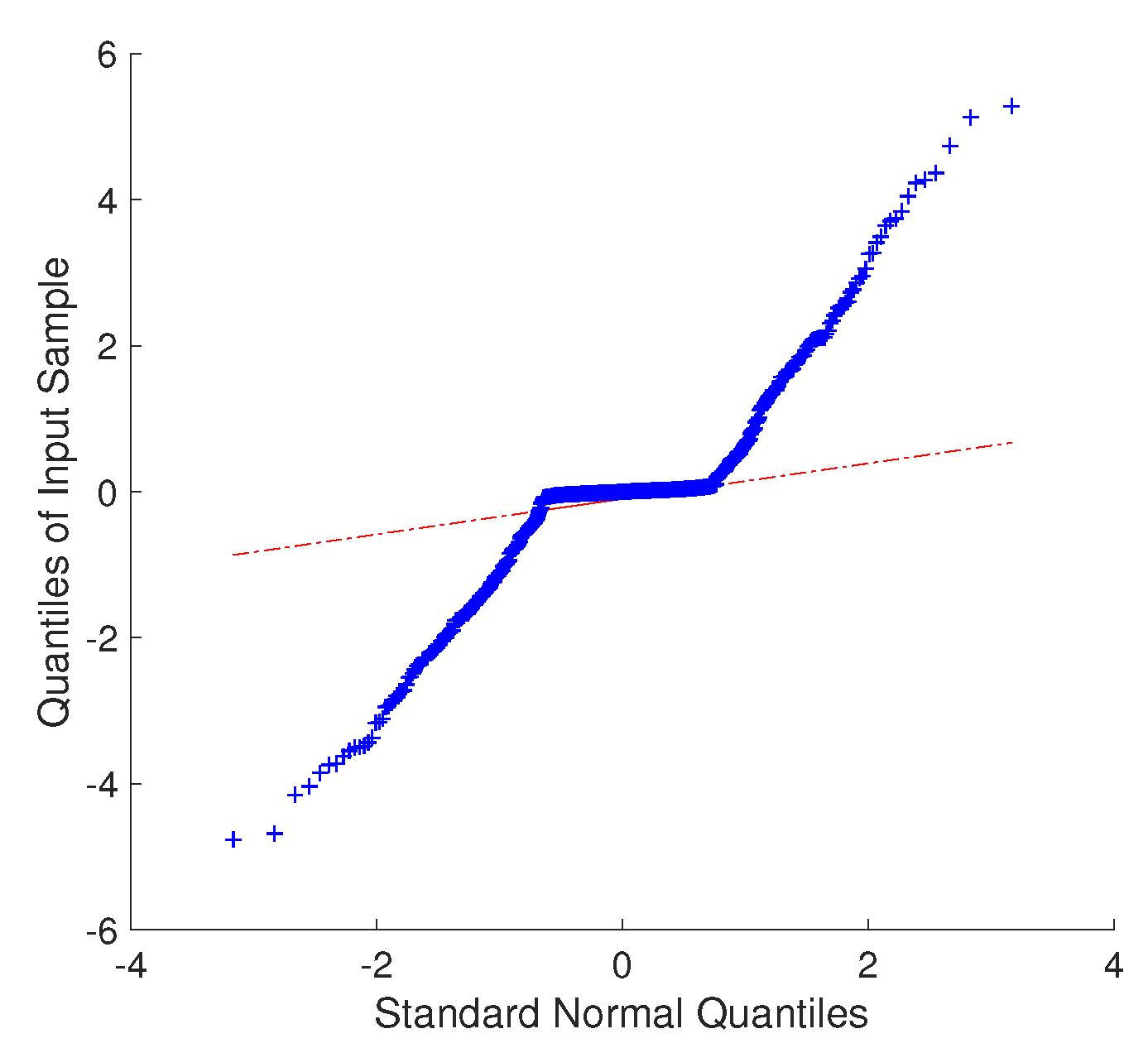
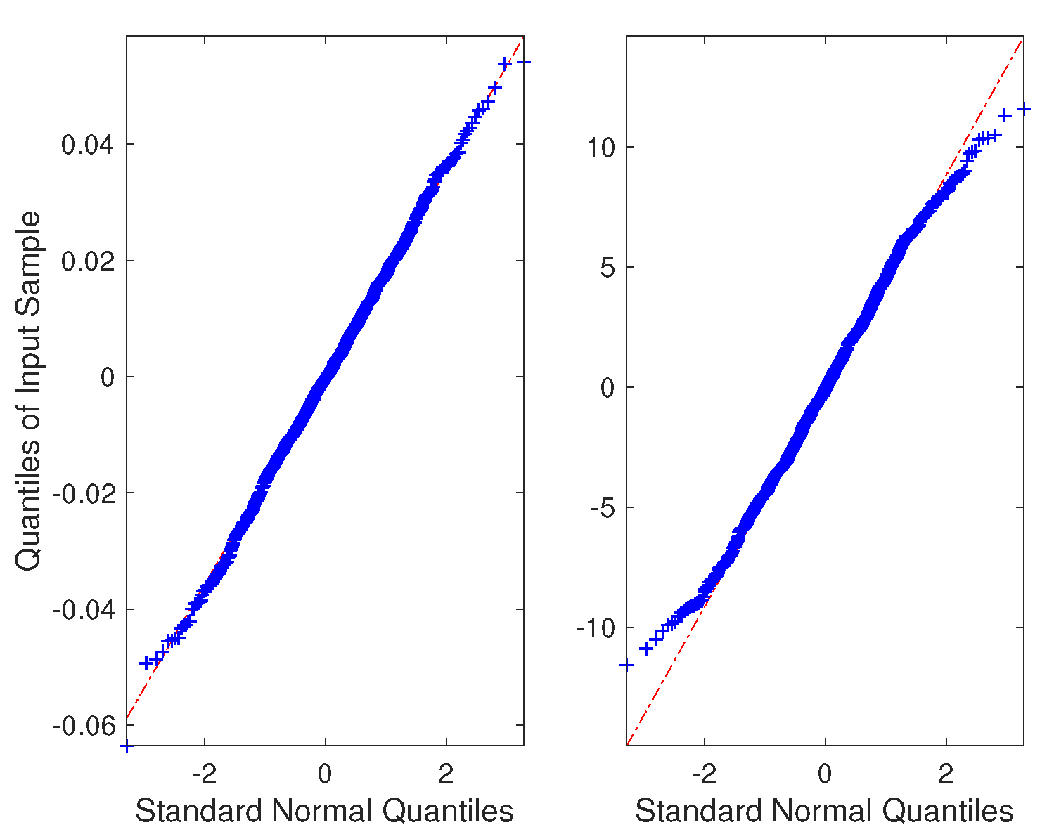
First, the residuals were analyzed. The QQ-plot for the residuals of the existing method are shown in Figure 5. The residuals do not appear to be distributed normally. This is caused by the design of the model in which all the parameters were evaluated using a single set of equations. The Y vector consisted of both Δ I and Δ V values. The magnitude of residuals for Δ I and Δ V is of different scales. Thus, the final residuals are made up of two data sets which are normally distributed with different variances. The uncertainty was given by the deviation calculated using Method 1. Since the assumptions b and d about heteroscedasticity and normality were invalid, the CIs of the parameters were not correct. The actual percentage error was calculated based on the known reference values of the parameters. However, in the field measurements, accurate reference would not be available. In that case, the computed CIs give the expected error in the parameter estimates. Thus, a comparison between the calculated CIs and actual percentage errors is presented in Table 2. To simplify the result analysis and comparison process, the CIs are mentioned as the percentage deviation from the expected value of the parameters.
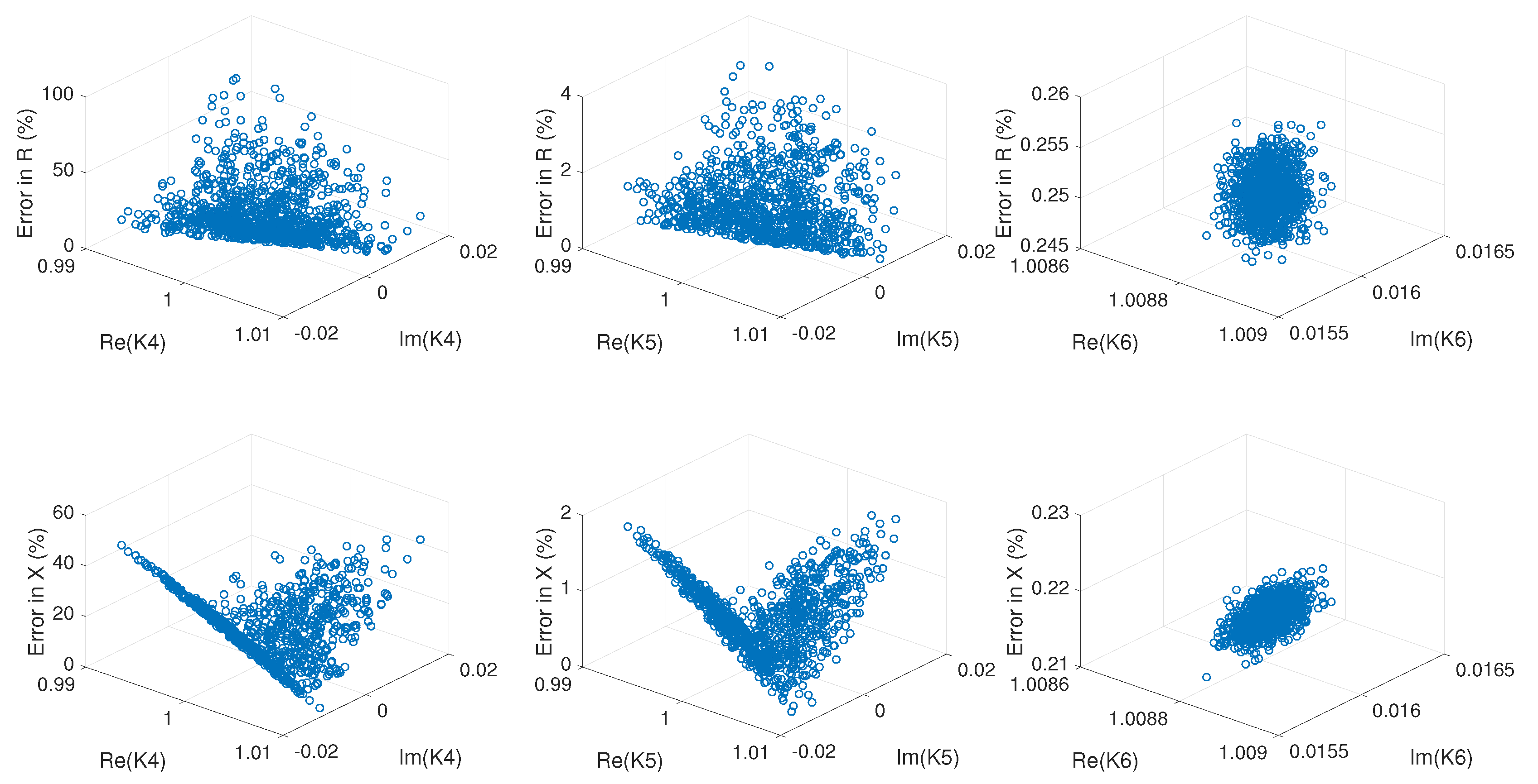
It is observed that the error in the estimates has increased in the presence of random errors in the phasor estimates. It was established that as there were no magnitude and phase errors in the CTs and VTs, the parameter estimates would be free from bias errors. Hence, the precision of the estimates given by the CI would be suggestive of the overall accuracy. However, for the existing method, the CIs for individual parameters are narrow and fail to include the actual error percentage.
In the proposed method, the two sets of Equations (12) and (13) are solved separately, and the two sets of residuals are obtained. Separate uncertainty estimates are calculated based on the statistical properties of both the equation sets. The QQ-plot for the residuals of the existing method are shown in Figure 6. It was observed by the plots that the residuals from both the subsystems appear to have a normal distribution. These plots validate that the system modeled by the equations sets is explained by the measurements and the calculated uncertainty limits can be trusted. Component-wise confidence intervals using Method 1 and Method 3 for the parameters estimated using the proposed method are presented in Table 3. Also presented are the actual error percentages associated with each parameter. For the sake of simplicity, the 3-phase cable simulated for the new method was modeled with no mutual susceptance. Norm-wise confidence interval using Method 2 and norm-wise actual errors in the parameters are presented in Table 4.
On comparing the results shown in Table 2 with the results shown in Table 3 and Table 4, two improvements can be observed. The absolute percentage error in the parameters caused by the random errors in measurements have been reduced by the new method. Secondly, the CI computed by the methods actually encompasses the absolute errors. However, as shown in Table 3, it was found that the CIs given by Method 3 are very wide compared to the actual percentage errors. Hence, Method 1 was selected to compute component-wise CI, and Method 2 was selected to compute norm-wise CI. The effect of fixed bias errors in the measurements on the parameter estimates is presented in Section 5.3.

5.3. Measurements with Only Fixed Bias Errors

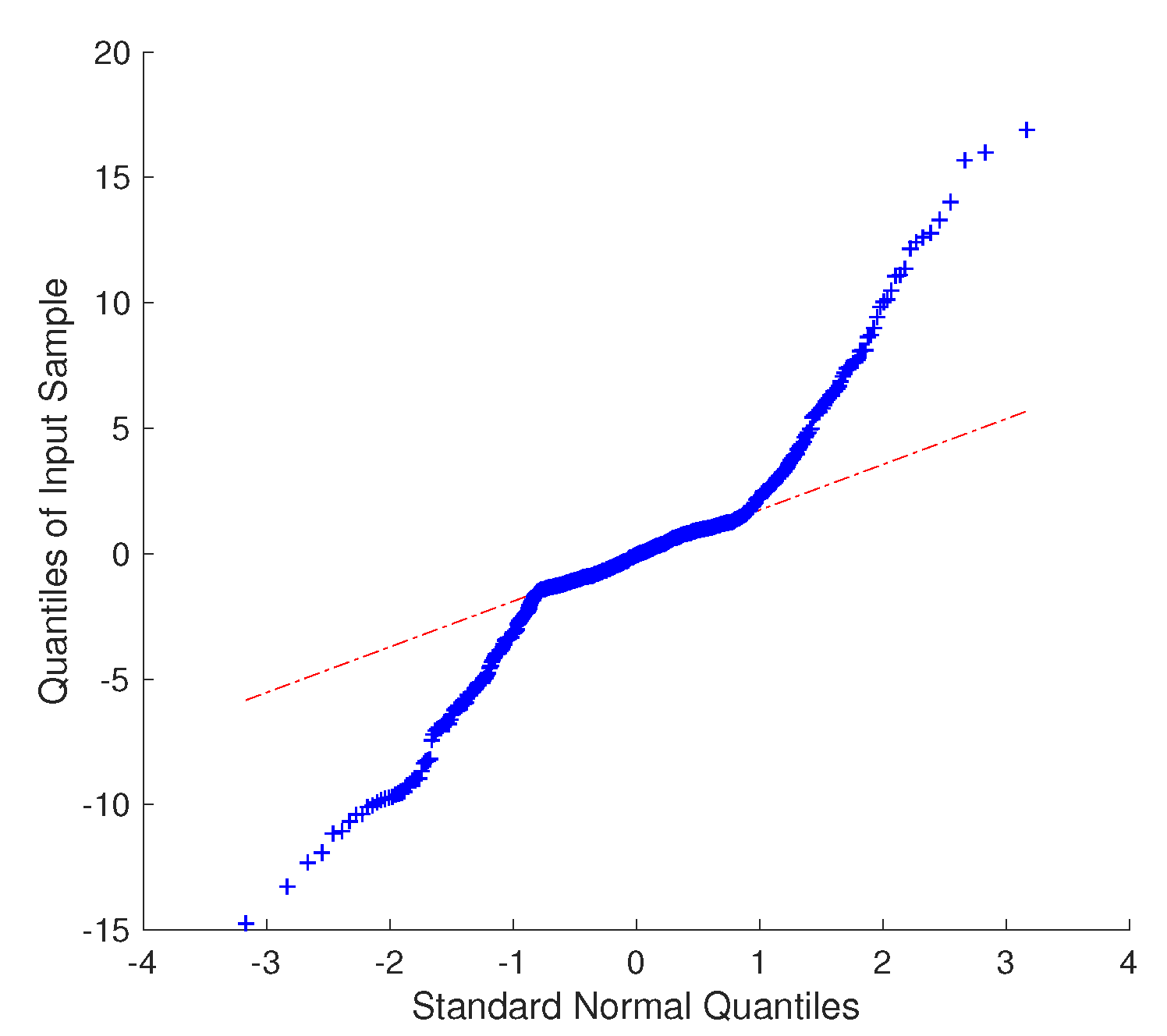
Class 1.0 CTs and VTs are used, and they are not calibrated. That means the correction coefficients are not known, and the actual magnitude and phase errors could be anywhere in the range of class 1.0 CTs and VTs. Thus, there was an unknown bias present in the used voltage and current measurements. No random noise errors were imposed on the measurements. The same power flow profile was used, and current and voltage signals were recorded and filtered. The data were fed to both methods, and cable parameters were estimated. The QQ-plots for residuals for both methods are plotted in Figure 7 and Figure 8. It was observed that the residuals obtained using the existing method do not appear to have a normal distribution. In comparison, the residuals obtained while estimating the parameters using the proposed method seem to have a better fit for a normal distribution. It is also observed the residuals from the proposed method are smaller in magnitude in comparison with the residuals from the existing method. These factors suggest that the proposed method gives better accuracy parameter estimates.
The CIs of parameters calculated using the existing method along with the actual errors are presented in Table 5. It can be seen that there is a significant difference between the estimated CIs and the actual errors of the parameters. For the proposed method, the uncertainty caused by the bias errors in the measurements is calculated as per Section 4.4 and is presented in Table 6. It was observed that the actual errors for all the parameters are enveloped by the CIs.
Table 2, Table 3, Table 4, Table 5 and Table 6 show the superiority of the new proposed line parameter estimation and the uncertainty computation methods. In the existing method, the residuals in the presence of bias errors and random noise appear to have a non-normal distribution, and as predicted, the accuracy of the estimated parameters is not in accordance with the calculated CIs. When compared to the reference value of the parameters, the estimated parameters were outside the CIs. The parameter estimates from the proposed method when compared to reference values were found to be more accurate. In field measurements, the actual reference could be unavailable or misleading. Hence, the CIs should be reliable and precise. The proposed method gave reliable and precise CIs in the presence of bias and random errors. After the comparison, Method 1 from Section 4.1 was chosen to estimate the uncertainty caused by the random errors and the uncertainty caused by bias errors in the measurements was estimated using the Monte Carlo-based method shown in Section 4.4. Combined uncertainty in terms of a CI was then calculated according to Equation (23).

5.4. Measurements with Both Random Noise and Bias Errors

In the final simulation test, both random and bias errors are simulated in the measurement system. The same power-flow in the cable was simulated, and hence, the same voltage and current signals were used. The results for both methods are presented in Table 7. The results are presented in terms of norm-wise CIs and norm-wise actual errors of the vectors of susceptance B and impedance R + j X parameters. For the existing method, it was observed that the parameter estimates were not accurate, and CIs were inaccurate and wide. Separate CIs to account the effects of random noise ( α ) and bias errors ( β ) in the measurements were computed for the parameters estimated by the proposed method. Combined CIs were calculated and compared with the actual errors. The parameters given by the proposed method were substantially more accurate, and the computed CIs were found to be reliable, enveloping the actual percentage error.
The next section presents the results of a test done in the university laboratory to estimate the impedance parameters of a low voltage (LV) distribution cable using the proposed method.

5.5. Laboratory Test with Random and Bias Errors

This test presents the performance of the proposed method in the presence of random and bias measurement errors in the sensors. The power quality laboratory at the university has a 4-core (3 phase + 1 Neutral) Al cable of a total cross-section area of 70 2 feeding a flexible power source to a number of household connections via short 16 2 (3 phase + 1 Neutral) Cu cables. The new proposed method was tested for its accuracy while estimating the impedance parameters of the combination of the Al cable and the Cu cable until the last household. The exact length of the main Al and smaller Cu cables was unknown. To set a reference, the DC resistance of the combined cable was calculated using several measurements at varying DC current levels from 1 A to 10 A. The DC current was measured by the and the voltage difference between the two ends of the cable was measured by high accuracy devices. The reference DC resistance between the two ends of the cable system was calculated to be 0.0935 Ω . For the parameter estimation test, time domain voltage waveforms were measured and digitally acquired at two ends of the line using two National Instruments NI-9225 voltage input modules based on cRIO-9038 chassis. The line current was measured by a rogowsky coil and acquired by an NI-9234 input module. All of the measurement signals were acquired with a sampling frequency of 25 kHz. All the input channels of the cRIO chassis were also time-synchronized with an accuracy of ± 200 ns. Bias associated with each individual component of the measurement chain was taken from the manufacturer’s specification sheet. This bias uncertainty associated with each equipment is presented in Table 8. These values are the maximum possible fixed deviations in the measured signals.
The combined bias in the measured current and voltage signals was estimated using Type B uncertainty calculation as suggested in the GUM. The absolute uncertainty of the individual component is computed as the sum of all of the associated errors for that device. Thus, for each component x, the uncertainty variance σ x 2 is calculated as the sum of its gain and offset errors. The combined uncertainty of two devices in a chain is given as the euclidean norm of the individual absolute uncertainty. For current measurement, the rogowski coil is used along with the NI-9234 acquisition block. Hence, the combined uncertainty in the current signals ( S D I ) due to bias in each of the components is given by:
S D I = σ r o g o w s k i 2 + σ N I 9234 2 .
The signals were converted into phasors using the DFT-based method. The combined bias in voltage and current phasors was calculated to be ± 0 . 058 % and ± 0 . 35 % , respectively. For the sake of simplicity, these bias errors were assumed to be solely magnitude errors of the CTs and VTs. These bias errors in the measure current and voltage signals were utilized to estimate the uncertainty in the resistance and reactance parameters of the cable.
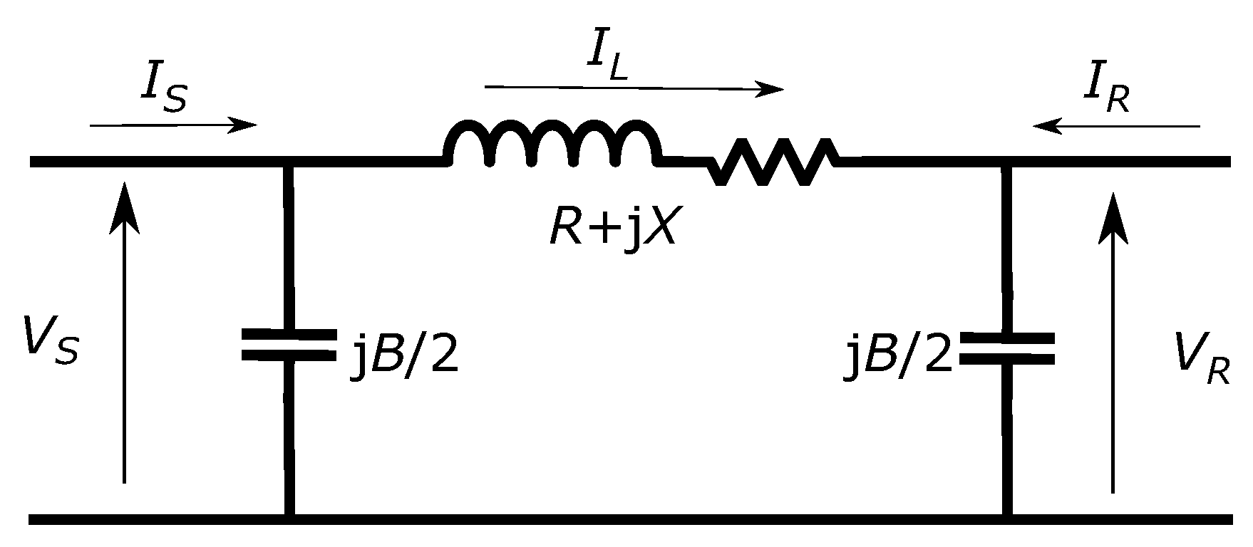
Since the length of the cables was very small, the effect of charging capacitance was ignored. Due to the small charging capacitance, there would not be any measurable difference between the current at two ends, and hence, current measurement was done only at one end and the current difference Equation (1) was ignored. Voltage and current phasors were calculated using the synchronized waveforms. Only the voltage difference in Equation (2) and hence, Equation (11) was used to make the system of linear equations. The 3-phase voltage difference equation can be written in matrix form as:
δ V a δ V b δ V c = r a a + j x a a r a b + j x a b r a c + j x a c r a b + j x a b r b b + j x b b r b c + j x b c r a c + j x a c r b c + j x b c r c c + j x c c * I a I b I c ,
that is :
δ V a b c = Z a b c * I a b c .
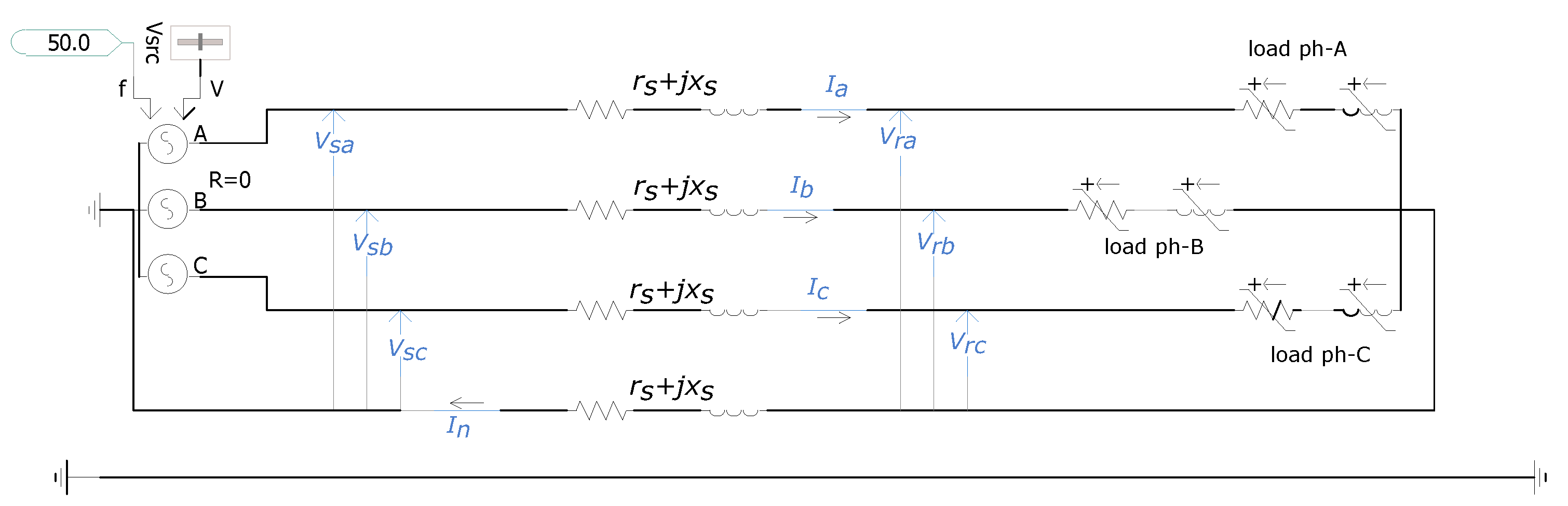
Figure 9 gives a basic overview of the laboratory cable and the measurement set-up. At the source end, there is a flexible and controllable voltage source and at the load end, there is a controllable load bank. The load bank was controlled to vary the load over a period of time. To facilitate the estimation of mutual reactance, a voltage drop due to the mutual reactance is required. Unbalanced loading of each phase excites the voltage drops due to mutual reactances. Hence, the load of each phase was kept different from each other. To model the laboratory cable, it was assumed that:
  • Self-impedance of all the three phases and the return path (neutral) is the same;
  • Self-resistance of single core of the cable (all phases and neutral) : r s ;
  • Self-reactance of single core of the cable (all phases and neutral) : x s ;
  • Mutual reactance coupling between all the phases is the same: x m ;
  • The mutual coupling effect of the neutral current on other phases is ignored.
The voltage difference equation can then be written with the help of parameters r s , x s , and x m . The current in neutral ( I n ) is the summation of I a , I b , and I c . These conditions make the voltage difference equations:
δ V a = I a * ( 2 r s + 2 j x s ) + I b * ( r s + j x s + j x m ) + I c * ( r s + j x s + j x m )
δ V b = I a * ( r s + j x s + j x m ) + I b * ( 2 r s + 2 j x s ) + I c * ( r s + j x s + j x m )
δ V c = I a * ( r s + j x s + j x m ) + I b * ( r s + j x s + j x m ) + I c * ( 2 r s + 2 j x s )
Using Equations (26)–(28), we can write the Z a b c in the form:
Z ˜ a b c = 2 r s + j 2 x s r s + j x ˜ m r s + j x ˜ m r s + j x ˜ m 2 r s + j 2 x s r s + j x ˜ m r s + j x ˜ m r s + j x ˜ m 2 r s + j 2 x s ,
where the effective mutual reactance in phasor form x ˜ m = x s + x m . Comparing Z ˜ a b c with Z a b c matrix, it can be seen that:
r a a = r b b = r c c = 2 r s ,
r a b = r b c = r a c = r s ,
x a a = x b b = x c c = 2 x s   and  
x a b = x b c = x a c = x ˜ m .
Thus, for accurate construction of the impedance matrix in phasor form ( Z a b c ) the parameters required to be estimated are: r s , x s a n d x ˜ m .
The existing and the proposed methods were used for estimation of parameters of the cable system. No correction coefficients for the bias present in the measurement sensors was applied in the model of Equation (9). Thus, for the proposed method, the model Equation (13) with adjusted correction coefficient K 4 
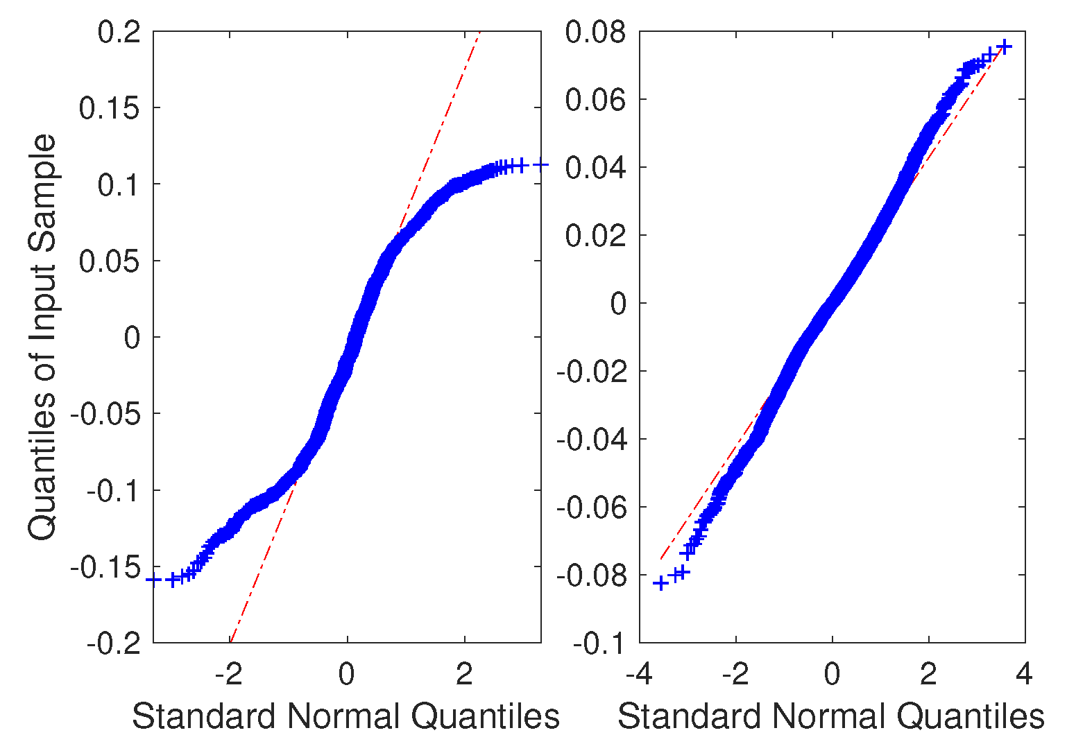
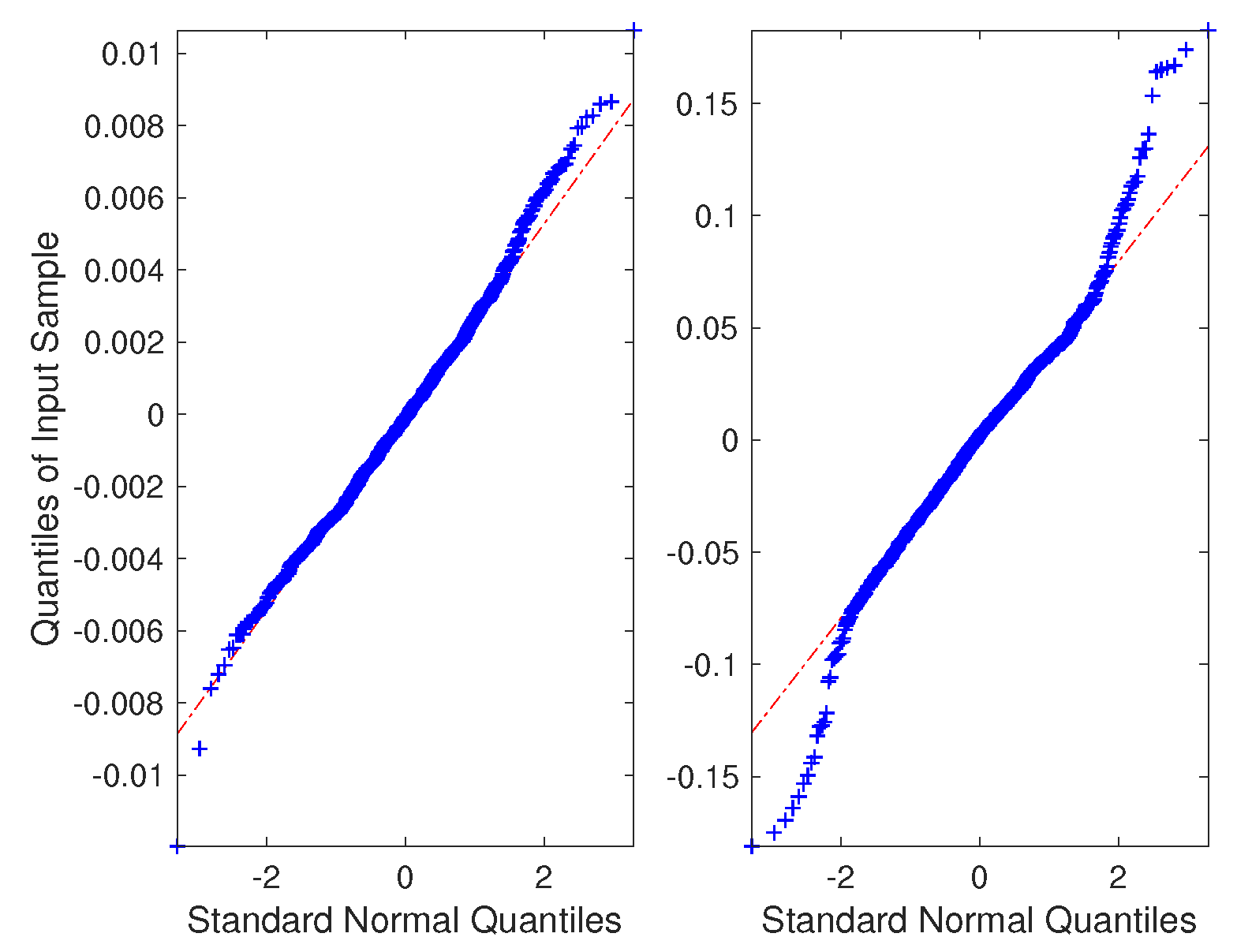
was utilized to estimate the impedance parameters. The QQ-plots of the residuals of the two methods are presented in Figure 10. The left side plot from the existing method does not appear to have a normal distribution. This indicates that there is an unaccounted bias error present in the measurement system. Comparison of the magnitude of the residuals from both the methods was done by comparing the ratio of euclidean norms of residuals (s) and the norms of corresponding measurement vector (Y). The ratio was 0.0721 for the existing method, while the new method resulted in a much smaller ratio of 1.0413 × 10 4 . The smaller norms ratio along with the QQ-plot comparison suggests that the results obtained from the proposed method are more accurate and have reliable uncertainty estimates when compared to the existing method. The results in terms of expected values and combined confidence intervals of the parameters are presented in Table 9.
The Z ˜ a b c matrix was composed with the estimated parameters using Equation (29). It was then converted into sequence components:
Z ˜ a b c = 0 . 190 + j 0 . 0216 0 . 095 + j . 0124 0 . 095 + j . 0124 0 . 095 + j 0 . 0124 0 . 190 + j . 0216 0 . 095 + j . 0124 0 . 095 + j 0 . 0124 0 . 095 + j . 0124 0 . 190 + j . 0216 , Z ˜ 012 = 0 . 380 + j 0 . 046 0 . 095 + j 0 . 009 0 . 095 + j 0 . 009 .
The positive sequence resistance is quite close to the reference value measured by the DC measurement system. Further, the fact that the zero sequence impedance is about four times the positive sequence impedance (especially for the resistance estimate) also suggests that the estimates are supporting the considered cable model. For a 3-phase 4-wire system with neutral as a return path, it is known that:
( r + j x ) 0 S e q = ( r + j x ) p h a s e + 3 * ( r + j x ) n e u t r a l
and in this case, ( r + j x ) p h a s e = ( r + j x ) n e u t r a l = ( r s + j x s ) . This validates the condition stated in Equation (30).
This subsection demonstrated the application of the proposed method for cable parameter estimation for an LV cable in a laboratory. A comparison with the results from the existing method was done to show the superiority of the proposed method. The next section presents some general discussion about the application of the proposed method in a real field.

6. Discussion

As no sensor comes without errors, it is important to estimate the performance of any application in their presence. The proposed method utilizes an overdetermined set of equations to estimate the parameters using OLS. The condition of the matrix H created using the available measurements could also play an important role in the quality of the results. The condition number κ for a full rank H matrix is a measure of uncertainty expected in the outcome of a mathematical operation on the matrix when its elements have errors. In short, it describes the sensitivity of the result obtained by an OLS estimator in the presence of the errors in the elements of the matrix H. A high condition number implies that the columns of the matrix H have a high correlation among them, making the matrix ill-conditioned. It is shown in [13] that the expected variance of the parameters ( θ i ) increases with increasing the correlation between the columns h i of the matrix H. Hence, applications like 3-phase parameter estimation which involve a high condition H matrix require high accuracy measurement set-ups. The columns of the matrix H are made up of the voltage and current measurements of different phases. The independence of voltage and current signals in different phases would result in lower correlation between the columns of the H matrix. Hence, for the application of any OLS-based method for cable parameter estimation in a 3-phase power system, apart from having high-quality sensors, some degree of independence in the power-flows in the three phases is required. The effect of correlation between power-flow in three phases on the accuracy of the proposed method is presented in Table 10. Two different sets of power-flows on the cable were simulated. All the other characteristics like measurement errors and data lengths were kept the same as in the previous simulation tests.
In Table 10, r P F is the mutual correlation coefficients between power-flow in the three phases, κ H is the condition number of the matrix H in corresponding power-flows, and N B and N Z are the norms of the calculated percentage errors in the B and Z parameter vectors. It is observed that with less correlation in the power-flow in three phases, the proposed method performs better and gives more accurate estimates. This realization could be used along with the idea presented in Section 4.2 to estimate the required accuracy of sensors for any application based on the prior knowledge about the condition of the matrix H for a given system and for a desired level of accuracy.
Another important consideration while estimating the parameters for any general system is realizing the underlying model of the system itself and designing the experiment for it. In the context of the laboratory cable experiment, to estimate the mutual reactance component x m , it is important to excite the mutual relationship between the current and the voltage signals. For this reason, the currents in three phases of the cable were kept different from each other by applying unbalanced loads. For balanced 3-phase conditions, the mutual components of the reactance might not be present, and using the same cable system model could give wrong results. Hence, modeling the system correctly is equally important for accurate and reliable parameter estimates.

7. Conclusions

This paper presents a new method for estimating the resistance, reactance, and susceptance (R, X and B) parameters for a 3-phase cable system. The new method is developed to facilitate accurate monitoring of cable temperature in real time to establish flexible loading levels of the cables [3]. The real-time cable temperature could be accurately estimated by tracking the real-time resistance of the cable. Hence, to estimate the cable temperature accurately, it is imperative to get high-accuracy resistance estimates. In the field, the temperature and hence the resistance of the cables vary continuously depending on the conditions, such as current magnitude, ambient soil temperature, and moisture content of the soil. There would be no correct reference to validate the estimated parameters, and thus, the calculation of the uncertainty of the resistance estimates is of equal importance. Hence, uncertainties in the estimated parameters are calculated accurately and presented as confidence intervals.
Using simulations and a laboratory test, it was shown that the regression model used in the proposed method can estimate these cable parameters with a better accuracy when compared to the existing method. The OLS-based proposed estimation method is sensitive to the errors in the measurement. The performance of the proposed method in the presence of random and bias measurement errors was investigated. To calculate the uncertainties of the estimates, new methods were presented and compared. It was shown that the total uncertainty is made up of two parts, one due to the random errors in the measurement and the second due to a fixed bias caused either by inherent bias in the measurement sensors or caused by errors in the used system model. The boundaries for deviations in the parameters were calculated when the measured signals had both random and fixed errors. It was also shown that utilization of a correct model of both the cable system and measurement chain is key to estimating the parameters more accurately and also estimating correct uncertainties. In the end, results from a laboratory test to estimate the parameter of a cable system were presented. The results from the laboratory test also showed that the proposed method was able to achieve more accurate and precise estimates in the presence of both random and bias errors in the sensors. The tests and the results showed that the proposed method is more suitable to estimate parameters of a 3-phase cable system in the field where the measurement equipment has unknown bias and random-error-related uncertainties.

Author Contributions

Conceptualization, R.S.S. and H.v.d.B.; Data curation, R.S.S. and S.B.; Investigation, R.S.S.; Methodology, R.S.S.; Project administration, V.Ć.; Supervision, S.C.; Writing—original draft, R.S.S.; Writing—review and editing, R.S.S., H.v.d.B., S.B., S.C., and V.Ć.

Funding

This work has received funding from the European Union’s Horizon 2020 research and innovation programme MEAN4SG under the Marie Skłodowska-Curie grant agreement 676042.

Conflicts of Interest

The authors declare no conflict of interest.The funders had no role in the design of the study; in the collection, analyses, or interpretation of data; in the writing of the manuscript, or in the decision to publish the results.

References

  1. Lee, J. Automatic Fault Location on Distribution Networks Using Synchronized Voltage Phasor Measurement Units. In Proceedings of the ASME 2014 Power Conference, Baltimore, MD, USA, 28–31 July 2014; pp. 1–5. [Google Scholar]
  2. Sachdev, M.S.; Agarwal, R. A technique for estimating transmission line fault locations from digital impedance relay measurements. IEEE Trans. Power Deliv. 1988, 3, 121–129. [Google Scholar] [CrossRef]
  3. Singh, R.S.; Cobben, S.; Gibescu, M.; van den Brom, H.; Colangelo, D.; Rietveld, G. Medium Voltage Line Parameter Estimation Using Synchrophasor Data: A Step Towards Dynamic Line Rating. In Proceedings of the 2018 IEEE Power Energy Society General Meeting (PESGM), Portland, OR, USA, 5–10 August 2018; pp. 1–5. [Google Scholar] [CrossRef]
  4. Shi, D.; Tylavsky, D.J.; Logic, N.; Koellner, K.M. Identification of short transmission-line parameters from synchrophasor measurements. In Proceedings of the IEEE 2008 40th North American Power Symposium, Calgary, AB, Canada, 28–30 September 2008; pp. 1–8. [Google Scholar] [CrossRef]
  5. Shi, D.; Tylavsky, D.J.; Koellner, K.M.; Logic, N.; Wheeler, D.E. Transmission line parameter identification using PMU measurements. Eur. Trans. Electr. Power 2011, 21, 1574–1588. [Google Scholar] [CrossRef]
  6. Ritzmann, D.; Wright, P.S.; Holderbaum, W.; Potter, B. A Method for Accurate Transmission Line Impedance Parameter Estimation. IEEE Trans. Instrum. Meas. 2016, 65, 2204–2213. [Google Scholar] [CrossRef]
  7. Ritzmann, D.; Rens, J.; Wright, P.S.; Holderbaum, W.; Potter, B. A novel approach to noninvasive measurement of overhead line impedance parameters. IEEE Trans. Instrum. Meas. 2017, 66, 1155–1163. [Google Scholar] [CrossRef]
  8. Milojević, V.; Čalija, S.; Rietveld, G.; Ačanski, M.V.; Colangelo, D. Utilization of PMU Measurements for Three-Phase Line Parameter Estimation in Power Systems. IEEE Trans. Instrum. Meas. 2018, 67, 2453–2462. [Google Scholar] [CrossRef]
  9. Menditto, A.; Patriarca, M.; Magnusson, B. Understanding the meaning of accuracy, trueness and precision. Accredit. Qual. Assur. 2007, 12, 45–47. [Google Scholar] [CrossRef]
  10. JCGM 100:2008, Evaluation of Measurement Data—Guide to the Expression of Uncertainty in Measurement; Joint Committee for Guides in Metrology: Sèvres, France, 2008.
  11. JCGM 102:2011, Evaluation of Measurement Data—Supplement 2 to the "Guide to the Expression of Uncertainty in Measurement; Joint Committee for Guides in Metrology: Sèvres, France, 2011.
  12. Khandeparkar, K.V.; Soman, S.A.; Gajjar, G. Detection and Correction of Systematic Errors in Instrument Transformers Along With Line Parameter Estimation Using PMU Data. IEEE Trans. Power Syst. 2017, 32, 3089–3098. [Google Scholar] [CrossRef]
  13. Greene, W.H. Econometric Analysis, 5th ed.; Pearson Education: London, UK, 2003. [Google Scholar]
  14. Golub, G.H.; Van Loan, C.F. Matrix Computations, 3rd ed.; The Johns Hopkins University Press: Baltimore, MD, USA, 1996. [Google Scholar]
  15. Higham, N. Accuracy and Stability of Numerical Algorithms, 2nd ed.; Society for Industrial and Applied Mathematics: Philadelphia, PA, USA, 2002. [Google Scholar] [CrossRef]
  16. Olive, D.J. Linear Regression; Springer International Publishing: Cham, Switzerland, 2017; p. 254. [Google Scholar] [CrossRef]
  17. Arbiter Systems, Inc. Model 1133a Power Sentinel Power Quality Revenue Standard Operation Manual; Arbiter Systems, Inc.: Paso Robles, CA, USA.
Figure 1. Nominal Pi model for a medium length medium voltage line.
Energies 12 04573 g001
Figure 2. Sensitivity of B with respect to coefficients K 1 , K 2 , and K 3 .
Energies 12 04573 g002
Figure 3. Sensitivity of R and X with respect to coefficients K 4 , K 5 , and K 6 .
Energies 12 04573 g003
Figure 4. Flowchart summarizing the process of accurate parameter estimation of a cable segment.
Energies 12 04573 g004
Figure 5. Existing Method: QQ-plot for the residuals in presence of random noise errors. Both sets of Equations (12) and (13) were solved together. Non-normal distribution and heteroscedasticity is observed.
Energies 12 04573 g005
Figure 6. Proposed Method: QQ-plot for the residuals in presence of random errors. The left plot shows residuals after solving (12) for B estimates. Right plot shows residuals after solving Equation (13) for R and X estimates.
Energies 12 04573 g006
Figure 7. Existing Method: QQ-plot for the residuals in presence of bias errors. Both sets of Equations (12) and (13) were solved together. Non-normal distribution and heteroscedasticity is observed.
Energies 12 04573 g007
Figure 8. Proposed Method: QQ-plot for the residuals in presence of bias errors. The left plot is for residuals after solving Equation (12) for B estimates. The right plot shows residuals from solving Equation (13) for R and X estimates.
Energies 12 04573 g008
Figure 9. Laboratory cable and measurement set-up.
Energies 12 04573 g009
Figure 10. Laboratory cable test: QQ-plot of the residuals for Equation (13) using the acquired data. Left plot: existing method, right plot: proposed method.
Energies 12 04573 g010
Table 1. Results using the existing method without any errors: Reference parameters and accuracy of both the methods when compared to the actual parameters. When no errors are present in the measurements, the proposed method uses the same system of equations and gives the same results.
PhaseResistance (R)Reactance (X)Susceptance (B)
Reference ( Ω )Error (%)Reference ( Ω )Error (%)Reference ( Ω 1 )Error (%)
A–A2.549 1 . 08 × 10 9 1.738 2 . 03 × 10 9 1.2 × 10 3 2 . 22 × 10 7
A–B1.592 1 . 82 × 10 9 0.066 5 . 43 × 10 8 2.1 × 10 6 1 . 22 × 10 4
A–C1.528 1 . 78 × 10 9 0.068 5 . 30 × 10 8 2.1 × 10 6 1 . 22 × 10 4
B–B2.551 1 . 04 × 10 9 1.738 2 . 06 × 10 9 1.2 × 10 3 2 . 22 × 10 7
B–C1.529 1 . 78 × 10 9 0.068 5 . 14 × 10 8 2.1 × 10 6 1 . 22 × 10 4
C–C2.548 1 . 08 × 10 9 1.734 2 . 04 × 10 9 1.2 × 10 3 2 . 22 × 10 7
Table 2. Existing method: Results in the presence of random noise errors. Discrepancy between computed confidence intervals (CIs) and actual errors is observed.
PhaseResistance (R)Reactance (X)Susceptance (B)
CI (%)Error (%)CI (%)Error (%)CI (%)Error (%)
A–A 1 . 09 2 . 30 0 . 84 0 . 96 964113
A–B 5 . 34 13 . 01 1 . 72 2 . 33 113 6 . 2 × 10 4
A–C 5 . 36 12 . 40 1 . 72 1 . 79 113 6 . 2 × 10 4
B–B 1 . 08 1 . 23 0 . 83 0 . 60 971113
B–C 5 . 30 14 . 45 1 . 74 0 . 58 113 6 . 2 × 10 4
C–C 1 . 10 2 . 69 0 . 84 0 . 86 965113
Table 3. Proposed method: Results in the presence of random noise errors in the measurements. Component-wise CIs using Method 1 (CI1) and Method 3 (CI3) and actual errors are presented. Computed CIs envelope the actual errors.
PhaseResistance (R)Reactance (X)Susceptance (B)
CI1 (%)CI3 (%)Error (%)CI1 (%)CI3 (%)Error (%)CI1 (%)CI3 (%)Error (%)
A–A1.0811.990.5701.5717.501.130.010.230.002
A–B1.4215.730.8534.15377.94.21---
A–C1.4415.960.3830.18333.810.63---
B–B1.1112.350.2701.6418.190.490.010.230.005
B–C1.4716.120.4930.14332.69.34---
C–C1.1112.320.3001.6318.000.340.010.230.001
Table 4. Proposed method: Results in the presence of random noise errors in the measurements. Norm-wise CIs using Method 2 (CI2) and actual errors are presented. Computed CIs envelope the actual errors.
EntityCI2 (%)Error (%)
R + j X 3.880.57
B0.230.003
Table 5. Existing method: Results in the presence of fixed bias errors in the measurements. Discrepancy between computed CIs and actual errors is observed.
PhaseResistance (R)Reactance (X)Susceptance (B)
CI (%)Error (%)CI (%)Error (%)CI (%)Error (%)
A–A 1 . 21 170 . 9 8 . 69 129 . 8 172 . 6 151 . 3
A–B 4 . 31 429 . 6 1 . 07 498 . 2 279 . 8 8 . 5 × 10 4
A–C 1 . 17 1 . 4 × 10 3 2 . 24 142 . 5 281 . 8 8 . 4 × 10 4
B–B 1 . 09 285 . 6 17 . 35 90 . 41 173 . 2 150 . 9
B–C 1 . 12 1 . 2 × 10 3 1 . 14 283 . 6 280 . 5 8 . 5 × 10 4
C–C 2 . 54 41 . 3 1 . 09 158 . 5 173 . 4 149 . 2
Table 6. Proposed method: Results in the presence of fixed bias errors in the measurements. Component-wise CIs and actual errors are presented. Computed CIs envelope the actual errors.
PhaseResistance (R)Reactance (X)Susceptance (B)
CI (%)Error (%)CI (%)Error (%)CI (%)Error (%)
A–A2.721.733.020.920.630.21
A–B1.180.8587.635.90--
A–C1.181.0277.635.58--
B–B2.692.044.471.890.690.60
B–C1.360.99112.243.29--
C–C2.932.313.861.900.570.25
Table 7. Comparison of results from the existing and the proposed method in the presence of both random and bias errors. The CIs are presented as the norm for the percentage deviation in the parameter vector. Errors in estimates from the proposed method are smaller, and the CIs are more accurate.
MethodParameters α (%) β (%) CI θ (%)Error (%)
Old MethodB--1.8 × 10 4 10.07
R + j X --75.0160.7
Proposed MethodB0.0260.6120.6130.395
R + j X 1.492.232.681.87
Table 8. Accuracy specifications of used measurement equipment.
EquipmentGain Error (%)Offset Error (%)
NI-9225 ± 0 . 05 ± 0 . 058
NI-9234 ± 0 . 05 ± 0 . 006
Rogowski Coil ± 0 . 3 ± 0 . 005
Table 9. Laboratory cable test: Expected parameters and corresponding CIs using both methods are presented. The ratio of norm of residuals to the norm of expected parameter is also presented.
Method r s ( Ω ) CI r s ( % ) x s ( Ω ) CI x s (%) x ˜ m ( Ω ) CI x ˜ m ( % ) | | s | | | | Y | |
Existing Method0.09660.320.01176.600.012012.800.0721
Proposed Method0.09510.470.01083.550.01244.821.0413 × 10 4
Table 10. Effect of conditioning of Matrix H.
r PF κ H N B (%) N Z (%)
[0.9801 0.9799 0.9794]7.94 × 10 3 0.4021.769
[0.9992 0.9996 0.9994]2.54 × 10 3 0.40318.495

