Numerical Modeling of CO₂, Water, Sodium Chloride, and Magnesium Carbonates Equilibrium to High Temperature and Pressure

Abstract

In this work, a thermodynamic model of CO₂-H₂O-NaCl-MgCO₃ systems is developed. The new model is applicable for 0–200 °C, 1–1000 bar and halite concentration up to saturation. The Pitzer model is used to calculate aqueous species activity coefficients and the Peng–Robinson model is used to calculate fugacity coefficients of gaseous phase species. Non-linear equations of chemical potentials, mass conservation, and charge conservation are solved by successive substitution method to achieve phase existence, species molality, pH of water, etc., at equilibrium conditions. From the calculated results of CO₂-H₂O-NaCl-MgCO₃ systems with the new model, it can be concluded that (1) temperature effects are different for different MgCO₃ minerals; landfordite solubility increases with temperature; with temperature increasing, nesquehonite solubility decreases first and then increases at given pressure; (2) CO₂ dissolution in water can significantly enhance the dissolution of MgCO₃ minerals, while MgCO₃ influences on CO₂ solubility can be ignored; (3) MgCO₃ dissolution in water will buffer the pH reduction due to CO₂ dissolution.

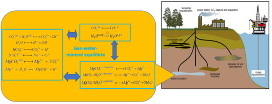
1. Introduction

CO₂ geological storage has been proved as an important option to reduce carbon emission and a clean way of using fossil energy resources [1]. When CO₂ is injected into underground reservoirs, the reactions of CO₂, water and various minerals are activated [2]. Magnesium carbonates are commonly found minerals in geological reservoirs. A reliable thermodynamic model of CO₂, brine, and magnesium carbonate minerals is essential to understand phase behavior, water property changes, and mineral participation and dissolution [3]. Further, it will help us to understand the reservoir property (porosity and permeability) change after CO₂ injected. Numerical dynamic simulation of the fluid migration process is usually an important tool to analyze the whole procedure and helps the decision making of a real CO₂ storage project [4]. The thermodynamic model is one of the basic components in a simulation framework.

Both magnesium and carbon are commonly found underground in terms of various kinds of minerals. Researchers started experimental work on the H₂O-MgCO₃ system in 1867 [5]. Wagner [5] measured magnesite solubility at 5 °C and with CO₂ partial pressure from 1 to 6 atm. The followers conducted magnesite solubility measurements with temperature up to 91 °C and CO₂ partial pressure up to about 10 atm [5,6,7,8,9,10,11,12]. Cameron and Seidel [12] measured magnesite solubility in NaCl solutions with NaCl molality up to 6.5 molal. Nesquehonite solubility in water was first measured by Engel et al. [13]. The most recent measurements were carried out by Konigsberger et al. [14]. The temperature range of the experiments is from 0–90 °C and CO₂ partial pressure ranges from about 0 to 56 atm [7,10,14,15,16,17,18]. Lansfordite solubility experiment work is less than magnesite and nesquehonite. The available literatures are Takahashi et al. [19], Ponizonvskii et al. [20], and Yanat’eva and Rassonskaya [21]. The temperature of the experiments is less than 15 °C and pressure is less than 10 atm. Numerical modeling of CO₂-brine-salts-minerals was started in the 1980s. The pioneer work is from Harvie and Weare [22] and Harvie et al. [23]. They developed series thermodynamic models of sea water components based on the Pitzer model [24,25,26,27]. The models are able to accurately predict mineral precipitation and dissolution. The temperature and pressure are at standard condition (25 °C and 1 atm). Moller [28], Moller and Greenberg [29], and Christov and Moller [30] modeled temperature effects on the system. Duan and co-workers focused on the pressure effects and developed models on CO₂-H2O-NaCl-CaCO₃-CaSO4 systems from standard condition to high temperatures and pressures [31,32,33,34]. Thermodynamic models have been implemented in research or commercial software on reactive transport. The most famous reactive transport software packages are PhreeqC [35], TOUGHREACT [36], MIN3P [37], and EQ3/6 [38]. They have shown success in real project applications [39,40,41]. Some commercial reservoir simulators have coupled the reactive transport module (such as CMG-GEM [42] and MoReS-PhreeqC [43]) and were successfully applied in enhanced oil recovery research or real projects [44,45].

In this work, a new thermodynamic model of CO₂-H₂O-NaCl-MgCO₃ systems is developed. The model is based on the existing experimental data and the consistency checking. The MgCO₃ minerals of magnesite, nesquehonite, and lansfordite are considered in the system. In Section 2, the methodology of the thermodynamic modeling is introduced. In Section 3, model validations are made by comparing the model results and available experimental data of the systems. In Section 4, the model is used to predict MgCO₃ mineral solubility, aqueous solution properties (such as pH and various carbon ion concentrations) at various conditions. The influences of CO₂ and MgCO₃ on the speciation in the solutions are evaluated by the model.

2. Phenomenological Description and Geochemical Modeling

When a system of CO₂-H₂O-NaCl-MgCO₃ approaches equilibrium at given temperature and pressure, phases of solids, vapor, and brine (aqueous phase) can appear. Minerals of magnesite (MgCO₃), nesquehonite (MgCO₃∙3H₂O), and lansfordite (MgCO₃∙5H₂O) are considered in this modeling work. The salt of sodium chloride (NaCl) can be precipitated when NaCl becomes saturated in the aqueous phase. In the vapor phase, the possible components are CO₂ and H₂O. In the aqueous phase, various cations, anions, and neutral particles can be dissolved. The following reversible reactions are considered for the modeling:

$${\mathrm{H}}_2{\mathrm{O}}^{(aq)}\stackrel{}{\leftrightarrow }{\mathrm{H}}_2{\mathrm{O}}^{(g)},$$

(1)

$${\mathrm{CO}}_2{}^{(aq)}\stackrel{}{\leftrightarrow }{\mathrm{CO}}_2{}^{(g)},$$

(2)

$${\mathrm{CO}}_2{}^{(aq)}+{\mathrm{H}}_2{\mathrm{O}}^{(aq)}\stackrel{}{\leftrightarrow }{\mathrm{CO}}_3{}^{2-}+2{\mathrm{H}}^{+},$$

(3)

$${\mathrm{H}}_2\mathrm{O}\stackrel{}{\leftrightarrow }{\mathrm{H}}^{+}+{\mathrm{OH}}^{-},$$

(4)

$${\mathrm{HCO}}_3{}^{-}\stackrel{}{\leftrightarrow }{\mathrm{CO}}_3{}^{2-}+{\mathrm{H}}^{+},$$

(5)

$${\mathrm{NaCl}}^{(s)}\stackrel{}{\leftrightarrow }{\mathrm{Na}}^{+}+{\mathrm{Cl}}^{-},$$

(6)

$${\mathrm{MgCO}}_3{}^{(s,Magnesite)}\stackrel{}{\leftrightarrow }{\mathrm{CO}}_3{}^{2-}+{\mathrm{Mg}}^{2+},$$

(7)

$${\mathrm{MgCO}}_3\cdot 3{\mathrm{H}}_2{\mathrm{O}}^{(s,Nesquehonite)}\stackrel{}{\leftrightarrow }{\mathrm{Mg}}^{2+}+{\mathrm{CO}}_3{}^{2-}+3{\mathrm{H}}_2\mathrm{O},$$

(8)

$${\mathrm{MgCO}}_3{·5\mathrm{H}}_2{\mathrm{O}}^{(s,Lansfordite)}\stackrel{}{\leftrightarrow }{\mathrm{Mg}}^{2+}+{\mathrm{CO}}_3{}^{2-}+5{\mathrm{H}}_2\mathrm{O},$$

(9)

$${\mathrm{MgCO}}_3{}^{(aq)}\stackrel{}{\leftrightarrow }{\mathrm{Mg}}^{2+}+{\mathrm{CO}}_3{}^{2-},$$

(10)

$${\mathrm{Mg}}^{2+}+{\mathrm{H}}_2\mathrm{O}={\mathrm{MgOH}}^{+}+{\mathrm{H}}^{+},$$

(11)

where (aq) denotes aqueous species; (s) denotes solid phase; (g) denotes gaseous phase species. When the whole system reaches equilibrium state, each of the above reactions will have:

$${\displaystyle \sum _r{\nu }_{ri}{\mu }_{ri}}=0,$$

(12)

where ${\mu }_{ri}$ is the chemical potential for reaction r and species i; ${\nu }_{ri}$ is the stoichiometric coefficient of species i in reaction r.

For aqueous species,

$${\mu }_i={\mu }_i^0+RT\ln (m_i{\gamma }_i).$$

(13)

For gaseous species,

$${\mu }_i={\mu }_i^0+RT\ln (x_{i}P{\phi }_i),$$

(14)

where ${\mu }_i^0$ is standard chemical potential at the reference state; $m_i$ is the molality of aqueous species i; ${\gamma }_i$ is the activity coefficient of aqueous species i; $x_i$ is mole fraction of gaseous species i; ${\phi }_i$ is fugacity coefficient of gaseous species i; P is total gas pressure; R is gas constant; T is temperature. More details about the parameter definition can be found from Duan and Li [32] and Li and Duan [34]. With Equations (12)–(14), equilibrium constant is usually defined for each chemical reaction as follows:

$$\ln K_r=-\frac{{\displaystyle \sum _i{\nu }_{ri}{\mu }_{ri}^0}}{RT}.$$

(15)

Combined with definition of chemical potential, we have:

$$K_r=\mathsf{\Pi }{a}_{ri}{}^{{\nu }_{ri}}$$

(16)

Here, $a_{ri}$ is activity for aqueous species ($m_r{}_i{\gamma }_{ri}$) and fugacity for gaseous phase ($x_{ri}P{\phi }_{ri}$). The thermodynamic modeling of the system is to determine the equilibrium constants, activity, and fugacity of each reaction. We follow the model from our previous work from Li et al. [46] for reactions (1) and (2), and from Li and Duan [34] for reactions (3) to (6).

2.1. Equilibrium Constant

The equilibrium constant can be further expressed as [33,34]:

$$K_i=K(T,P_{ref})\exp \left(\frac{\overline{V_{m,i}}(P-P_{ref})}{RT}\right),$$

(17)

where $K(T,P_{ref})$ is equilibrium constant at reference pressure $P_{ref}$; the reference pressure is usually 1 bar at temperature under 373.15 K, and vapor pressure of water above 373.15 K; $\overline{V_{m,i}}$ is molar volume of aqueous species i. For $K(T,P_{ref})$, we follow the empirical equation from Appelo [47]:

$$\log (K_H(T,P_{ref}))=A_0+A_{1}T+\frac{A_2}{T}+A_3\log (T)+\frac{A_4}{T^2}+A_5{T}^2.$$

(18)

For reactions (7) to (9), we regressed the parameters in Equation (17) and $\overline{V_{m,i}}$ from the related mineral solubility in water or brine. $\overline{V_{m,i}}$ is calculated as follows:

$$\overline{V_{m,i}}=41.84\left(0.1a_{1,i}+\frac{100a_{2,i}}{2600+P}+\frac{a_{3,i}}{(T-288)}+\frac{{10}^4{a}_{4,i}}{(2600+P)(T-288)}-{\omega }_i\times QBrn\right),$$

(19)

where a_1,i–a_4,i and ω_i are the parameters found in Appelo [47], and QBrn is the Born function, which can be found in Helgson et al. [48]. For magnesium carbonate dissolution reactions (7–9), we assume $\overline{V_{m,i}}$ is set as a constant value. For reactions (10) and (11), $\overline{V_{m,i}}$ is calculated following Helgson et al. [48].

Table 1. Parameters of equilibrium constants for magnesium carbonate dissolution reactions.

Reaction	A0	A1	A2	A3	A4	A5	$\overline{{\mathit{V}}_{\mathit{m}}}$
(7)	7.267	−0.033918	−1476.604	0	0	0	28.3
(8)	−6.008	−0.00688	873.4	0	0	0	74.789
(9)	−4.85	0	0	0	0	0	100.81
(10)	−0.5837	−9.2067	−2.3984	−0.03	0	0	Helgson et al. [48]
(11) a	−11.809	0	0	0	0	0	0

^a From Appelo [47].

shows the parameters used in this model.

2.2. Activity Model and Fugacity Model

From Equation (13), the activity coefficient describes the deviation of an aqueous species in a real solution from that in ideal solution. Pitzer [24] proposed an accurate model framework that can accurately estimate the activity coefficients of aqueous species and osmotic coefficients of H2O in solutions to high salinity. Science 1980s, the Pitzer model [24] framework began to be used to model water–salt–mineral equilibria with various kinds of aqueous species (Harvie and Weare [22]; Harvie et al. [23]; Greenburg et al. [29]; Moller [28]; Christov and Moller [30]; Li and Duan [33]) and shows its success in applications. Li and Duan [34] and many other literatures [29,30,31,32,33] provided the expressions of the model in details. In this work, we use the Pitzer model to calculate the activity coefficients. The Pitzer parameters includes cation and anion binary interaction parameters ${\beta }_{c,a}^{(0)}$, ${\beta }_{c,a}^{(1)}$, $C_{c,a}^{\phi }$, cation and cation binary interaction parameters ${\theta }_{c,c}$, anion and anion interaction parameters ${\theta }_{a,a}$, triple particle interaction parameters ${\Psi }_{c,c,a}$, ${\Psi }_{c,a,a}$, and neutral-ion interaction parameters ${\lambda }_{n-a}$, ${\lambda }_{n-c}$. The selection of the Pitzer parameters can be found from

Table 2. The Pitzer parameters of the system.

${\beta }_{C{O}_3^{2-},N{a}^{+}}^{\left(0\right)}$, ${\beta }_{HC{O}_3^{-},N{a}^{+}}^{\left(0\right)}$, ${\beta }_{C{l}^{-},N{a}^{+}}^{\left(0\right)}$, ${\beta }_{C{l}^{-},N{a}^{+}}^{\left(1\right)}$, ${\beta }_{C{O}_3^{2-},N{a}^{+}}^{\left(1\right)}$, ${\beta }_{HC{O}_3^{-},N{a}^{+}}^{\left(1\right)}$, ${\beta }_{O{H}^{-},N{a}^{+}}^{\left(0\right)}$, ${\beta }_{O{H}^{-},N{a}^{+}}^{\left(1\right)}$, $C_{C{O}_3^{2-},N{a}^{+}}^{\phi }$, $C_{HC{O}_3^{-},N{a}^{+}}^{\phi }$, $C_{C{l}^{-},N{a}^{+}}^{\phi }$, $C_{O{H}^{-},N{a}^{+}}^{\phi }$, ${\Psi }_{C{l}^{-},HC{O}_3^{-},N{a}^{+}}$, ${\Psi }_{C{l}^{-},O{H}^{-},N{a}^{+}}$, ${\Psi }_{C{l}^{-},H^{+},N{a}^{+}}$	Li and Duan [33], Duan and Li [32]
${\beta }_{C{O}_3^{2-},M{g}^{2+}}^{\left(0\right)}$, ${\beta }_{HC{O}_3^{-},M{g}^{2+}}^{\left(0\right)}$, ${\beta }_{C{l}^{-},M{g}^{2+}}^{\left(0\right)}$, ${\beta }_{C{l}^{-},M{g}^{2+}}^{\left(1\right)}$, ${\beta }_{C{O}_3^{2-},M{g}^{2+}}^{\left(1\right)}$, ${\beta }_{HC{O}_3^{-},M{g}^{2+}}^{\left(1\right)}$, ${\beta }_{O{H}^{-},M{g}^{2+}}^{\left(0\right)}$, ${\beta }_{O{H}^{-},M{g}^{2+}}^{\left(1\right)}$, $C_{C{O}_3^{2-},M{g}^{2+}}^{\phi }$, $C_{HC{O}_3^{-},M{g}^{2+}}^{\phi }$, $C_{C{l}^{-},M{g}^{2+}}^{\phi }$, $C_{O{H}^{-},M{g}^{2+}}^{\phi }$, ${\Psi }_{C{l}^{-},HC{O}_3^{-},M{g}^{2+}}$, ${\Psi }_{C{l}^{-},O{H}^{-},M{g}^{2+}}$, ${\Psi }_{C{l}^{-},H^{+},M{g}^{2+}}$	Greenburg et al. [29]; Moller 1988 [28] Christov and Moller [30];
${\Psi }_{C{l}^{-},O{H}^{-},Mg{\left(OH\right)}^{+}}$, ${\Psi }_{C{l}^{-},H^{+},Mg{\left(OH\right)}^{+}}$, ${\beta }_{C{l}^{-},Mg{\left(OH\right)}^{+}}^{\left(0\right)}$, ${\beta }_{C{l}^{-},Mg{\left(OH\right)}^{+}}^{\left(1\right)}$, ${\beta }_{HC{O}_3^{-},Mg{\left(OH\right)}^{+}}^{\left(0\right)}$, ${\beta }_{C{O}_3^{2-},Mg{\left(OH\right)}^{+}}^{\left(1\right)}$	Set to 0.0
${\lambda }_{CO2,N{a}^{+}}$, ${\lambda }_{CO2,M{g}^{2+}}$, ${\lambda }_{CO2,CO{3}^{2-}}$, ${\lambda }_{CO2,HC{O}_3{}^{-}}$	Duan and Sun [31]; Duan et al. [49]

.

To calculate the fugacity coefficient of gaseous component (CO₂ and H₂O), the Peng–Robinson (PR) model [50] is used. The details of the PR model and the methodology of the application are discussed in our previous work [2,46]. The equation for PR model is as follows:

$$P=\frac{RT}{V_m-b}-\frac{a(T)}{V_m(V_m+b)+b(V_m-b)}$$

(20)

where $a(T)=a(T_c)\alpha (T_r,\omega )$; a(T_c) is the Van der Waals’ attraction factor at a critical temperature defined as $a(T_c)=0.45724\frac{R^2{T}_c^2}{P_c}$, where P_c is critical pressure; $b=0.07780\frac{R{T}_c}{P_c}$; $T_r$ is reduced temperature $T_r=\frac{T}{T_c}$; $T_c$ is critical temperature; $\omega$ is acentric factor; $\alpha (T_r,\omega )$ is a dimensionless function of relative temperature and acentric factor.

When gaseous phase has more than one component, the mixing rule is considered for parameters “a” and “b”:

$$a={\displaystyle \sum _i{\displaystyle \sum _j{y}_i{y}_j{a}_{ij}}},$$

(21)

$$b={\displaystyle \sum _i{b}_i{y}_i},$$

(22)

where $a_{ij}=\sqrt{a_i{a}_j}(1-{\delta }_{ij})$ and ${\delta }_{ij}$ is binary interaction coefficient of species i and j; y_i is mole fraction of species i in gaseous phase. The PR parameters are adopted from Li et al. [46].

2.3. Calculation Routine

The equilibrium of the whole system is described by equations of chemical potentials, charge and mass conservation. The equations are non-linear. In this work, we use successive substitution method (Li and Duan [34]; Michealson and Mollerup [51]). The calculation routine is as follows.

(1)

Initialize the system with molality of each component and species at given pressure and temperature.

(2)

Calculate the equilibrium constant of each reaction.

(3)

Calculate activity coefficient of each aqueous species and fugacity coefficient of each gaseous species with current molality of each species of the system.

(4)

Solve mass and charge conservation equations and linearized reaction equilibrium equations. Update the molality and activity/fugacity coefficient of each species.

(5)

Calculate the absolute relative difference of molality of each species and activity coefficient. If both are smaller than tolerance, stop the calculation and output the final results. Otherwise, go to step (3).

3. Results

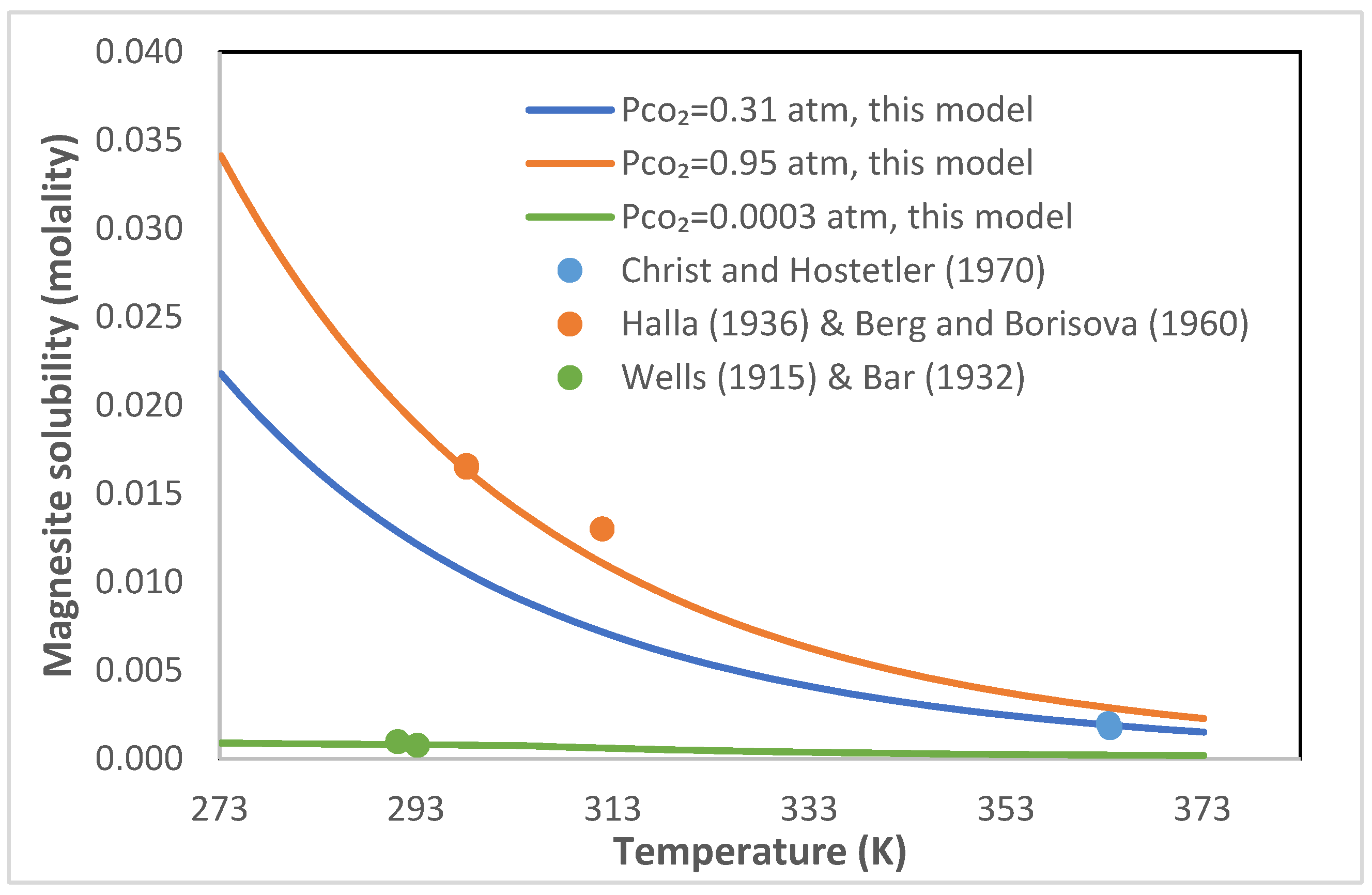
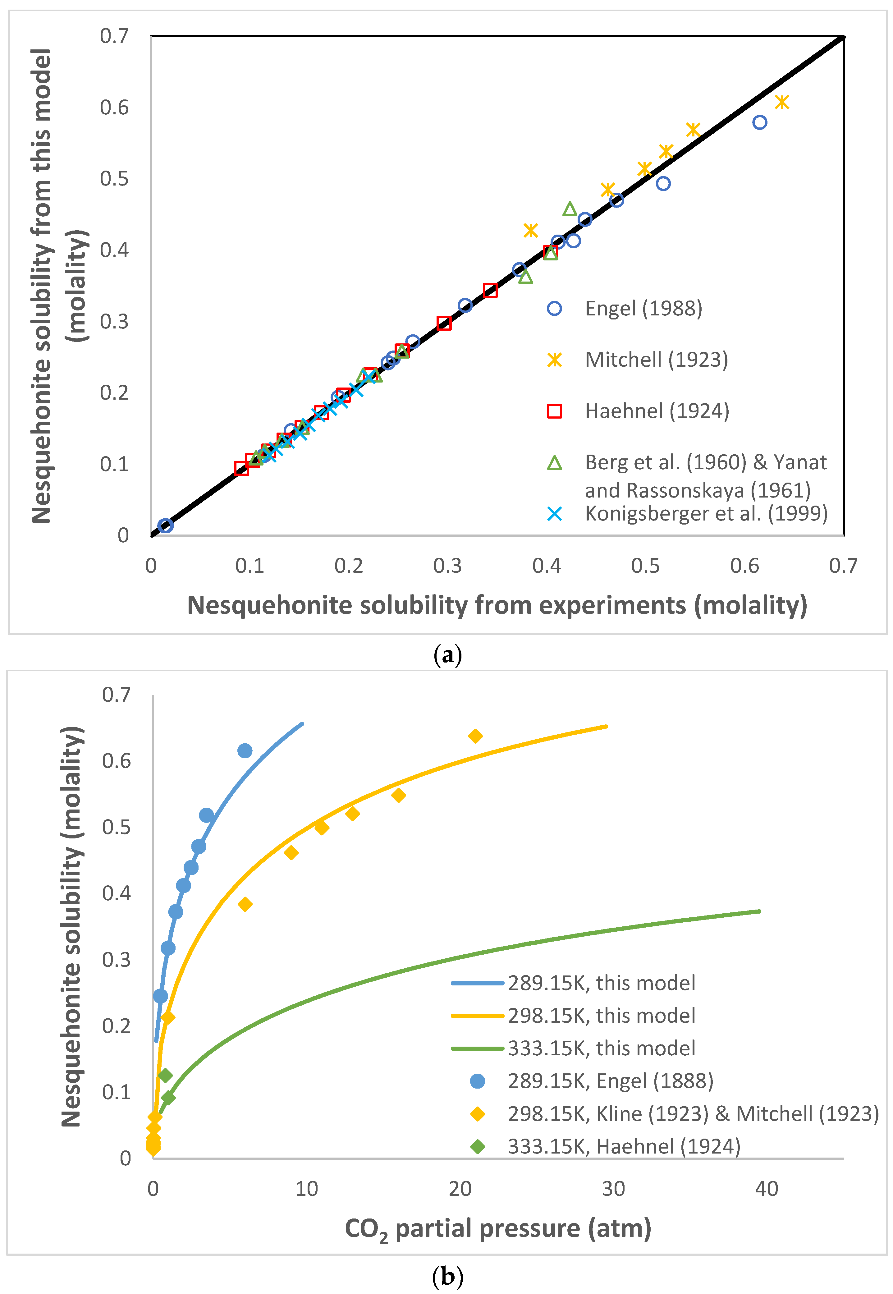
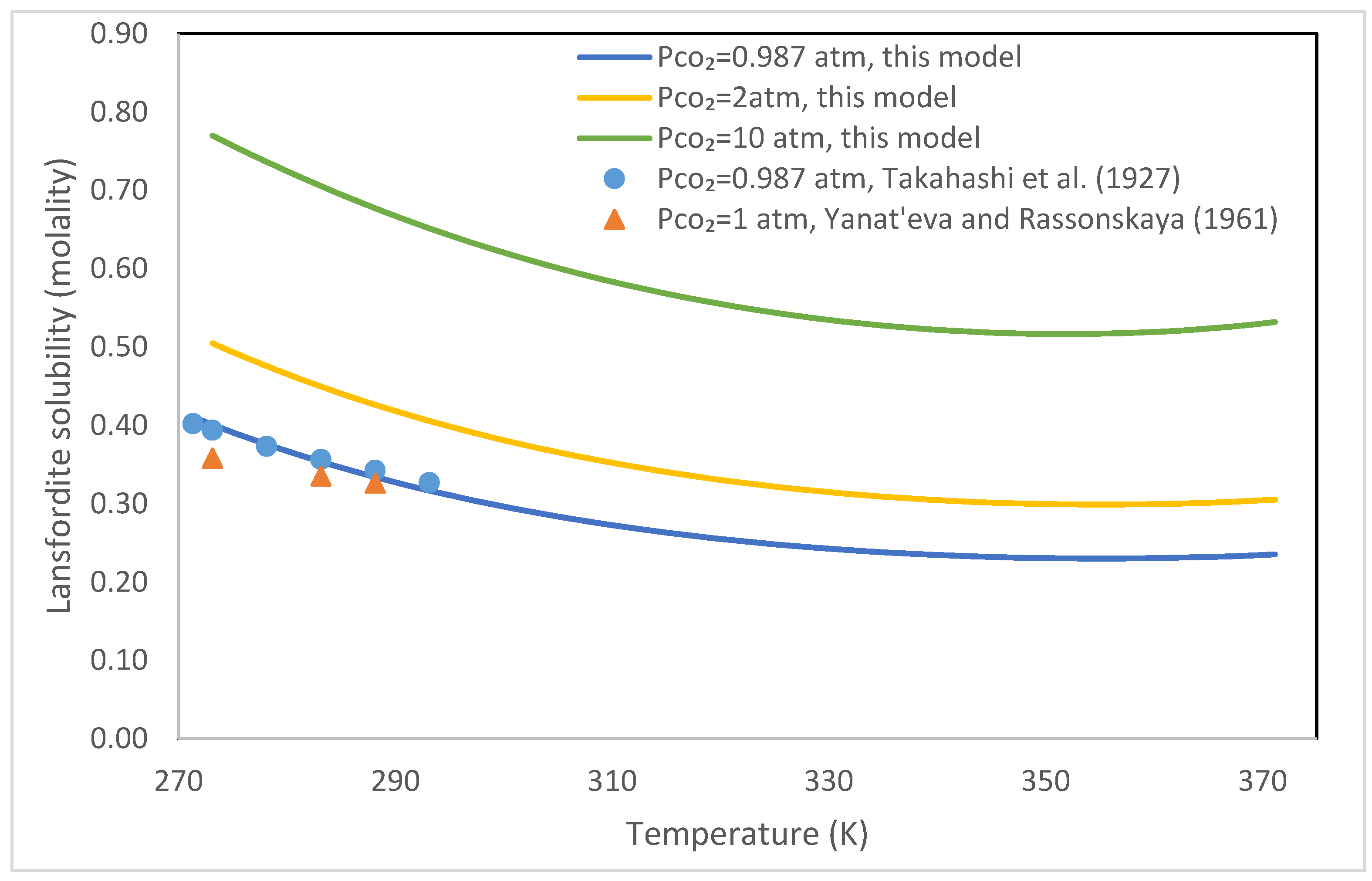
3.1. Comparisons of MgCO₃ Mineral Solubility: Model Calculations and Experiments

The experimental work of MgCO₃ mineral solubility started very early by previous researchers [5,6,7,8]. However, the reliable experimental data of this system is not sufficient for modeling. To test the model behavior, we compared the model results with the existing experimental data of MgCO₃ mineral solubility. Visscher et al. [52] carefully compared the experimental data and checked the reliability of the data. We defined average absolute deviation (AAD) to measure the difference between model results and experimental work:

$$AAD\%=\frac{1}{N}{\displaystyle \sum \left|\frac{s_{cal}-s_{\exp }}{s_{\exp }}\right|}\times 100\%,$$

(23)

where N denotes the number of data points; S_cal denotes calculated solubility; S_exp denotes experimental solubility.

Table 3. Average absolute deviation of magnesite solubility in water between model calculation by this model and the experimental results.

Reference	Data Points	T (°C)	PCO2 (atm)	AAD%
Wells [7]	1	20	0.00029	3.8
Bar [8]	2	18	0.00031	13.3
Halla [9]	2	25–38.8	0.932–0.955	8.75
Berg and Borisova [10]	1	25	0.987	11.6
Christ and Hostetler [11]	3	90.3–91	0.0274–0.312	9.61
Benezeth et al. [3]	11	120–200	12–30	13.17

shows the experimental data of magnesite (MgCO₃) in water and the average absolute deviation of the calculated results from this model. The experimental data of magnesite are usually at temperature from normal temperature to 91 °C and CO₂ partial pressure to about 1 atm. More recent work is from Benezeth et al. [3] who conducted experiments of magnesite solubility with temperature from 120 to 200 °C and CO₂ partial pressure from 12–30 bar. From the comparison, the AAD% is usually less than 10% with some of them up to 13.17%. Figure 1 shows the magnesite solubility trend with temperature at various CO₂ partial pressure calculated by this model. The trend shows that the model results are reliable compared with the experimental data.

The experimental data of nesquehonite solubility in water is more than that of magnesite, but is with limited TP range. The temperature is from 0 to 60 °C and CO₂ partial pressure is from 0.00029 to 21 atm.

Table 4. Average absolute deviation of nesquehonite solubility in water between model calculation by this model and the experimental results.

Reference	Data Points	T (°C)	PCO2 (atm)	AAD%
Engel [13]	14	3.5–50	0.878–5.986	2.09
Wells [7]	2	20	0.00029	9.41
Mitchell [16]	6	25	6–21	5.22
Haehnel [17]	12	5–60	1	1.13
Yanat and Rassonskaya [21]	10	0–53.5	1	2.91

shows the comparison between experimental data and the calculated results by this model. The average absolute deviations are all under 10%. Figure 2a posts all of the experimental data (which are judged as reliable by Visscher et al. [52]) and the calculated results with dots, most of which are quite close to the equal line (y = x). Figure 2b shows the nesquehonite solubility varying with CO₂ partial pressure at various temperature. The comparison shows a reliable nesquehonite solubility trend with CO₂ partial pressure with this model calculations.

Compared with magnesite and nesquehonite, the experimental data of lansfordite solubility in water is even less. The experimental work covers the temperature range from −1.8 to 20 °C and CO₂ partial pressure from 1–10 atm.

Table 5. Average absolute deviation of lansfordite solubility in water between model calculation by this model and the experimental results.

Reference	Data Points	T (°C)	PCO2 (atm)	AAD%
Takahashi et al. [19]	6	−1.8–20	0.987	1.84
Ponizonvskii et al. [20]	4	0	1.93–9.68	3.92
Yanat’eva and Rassonskaya [21]	3	0–15	1	7.11

shows the average absolute deviation of the calculated results with this model from the current available experimental data. From the comparison, the calculated results are close to the experimental data. Figure 3 shows the lansfordite solubility varying with temperature at various CO₂ partial pressures. The available experimental data points are also post on the figure. The model results show its reliability to predict the solubility trend.

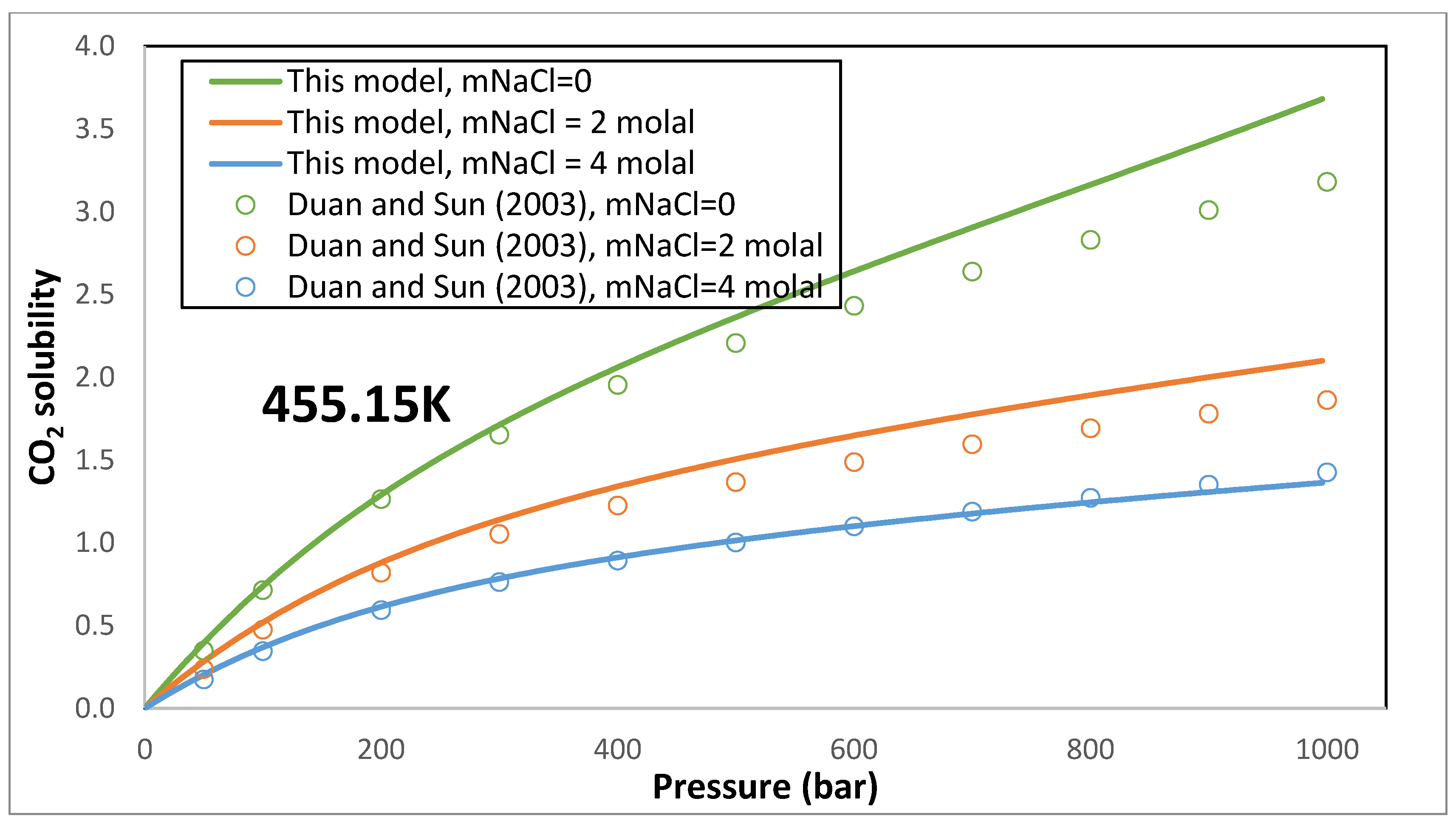
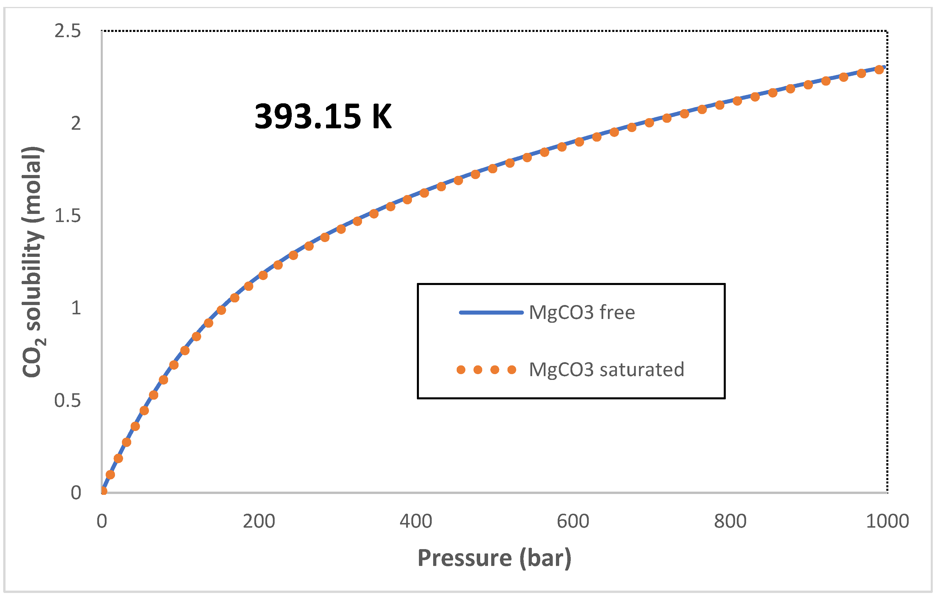
3.2. CO₂ Solubility

A complex system model should be able to reproduce experimental results of simple systems. Duan and Sun [31] developed an accurate model (DS model) for CO₂ solubility in water or brine within a wide pressure, temperature, and salinity range. DS model has been comprehensively examined with existing experimental data and is usually treated as a reliable model. We compared this model results for CO₂ solubility with DS model with temperature from 0–250 °C, pressure from 1–1000 bar, and NaCl molality from 0 to saturated condition. Figure 4 shows the comparisons between results from this model and the DS model. From the comparison, this model can reproduce the DS model results with wide TP range at different NaCl concentrations.

To evaluate the influences of MgCO₃ dissolution on CO₂ solubility in brine, numerical experiments are conducted with cases of MgCO₃ saturated solutions or MgCO₃ free solutions at various temperatures and pressures. Figure 5 shows the CO₂ solubility in water with MgCO₃ saturated or free conditions. From the comparisons, it can be concluded that dissolution of MgCO₃ in water has little influence on CO₂ solubility. This is because of the limited solubility of MgCO₃ minerals.

3.3. Model Predictions

With the new model, the following results can be calculated: (1) the solubility of MgCO₃ minerals (i.e., lansfordite, magnesite, and nesquehonite) at various conditions; (2) solutions properties such as pH, various ion concentrations and carbonate concentrations at various conditions of H2O-NaCl-MgCO₃-CO₂ systems.

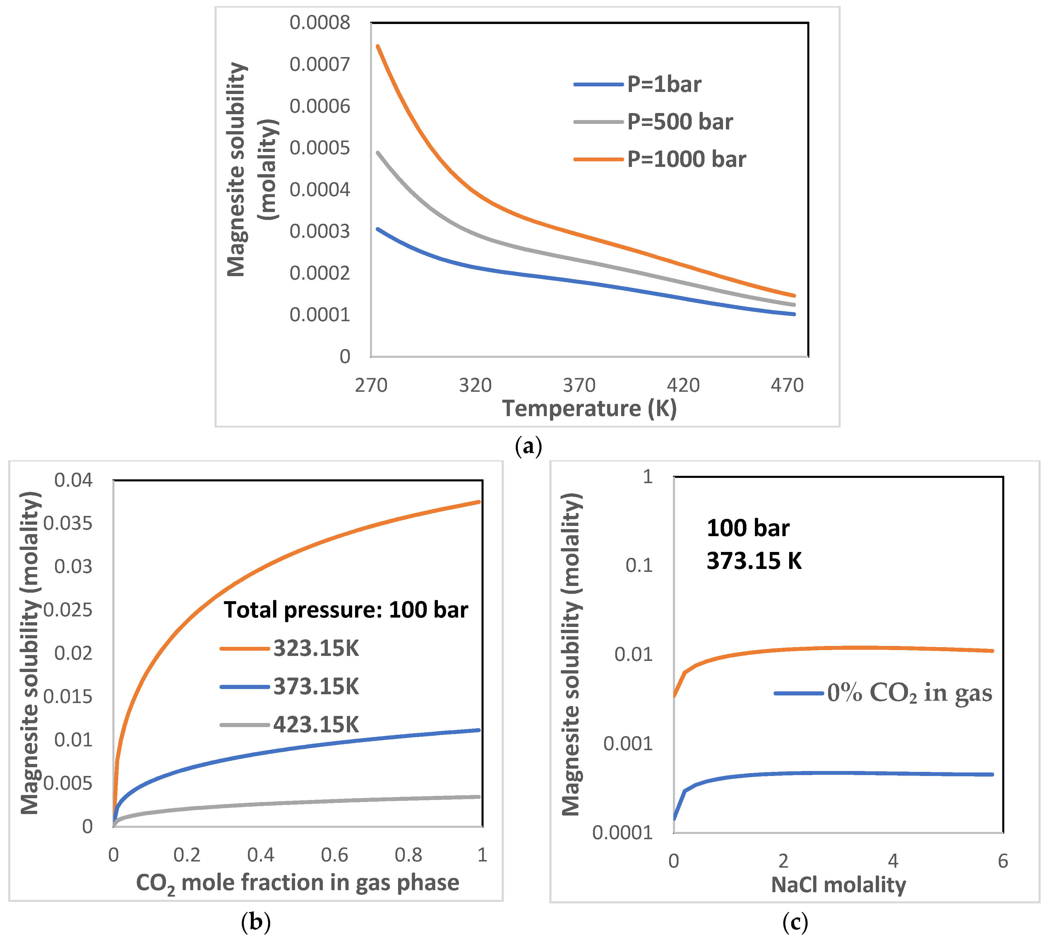
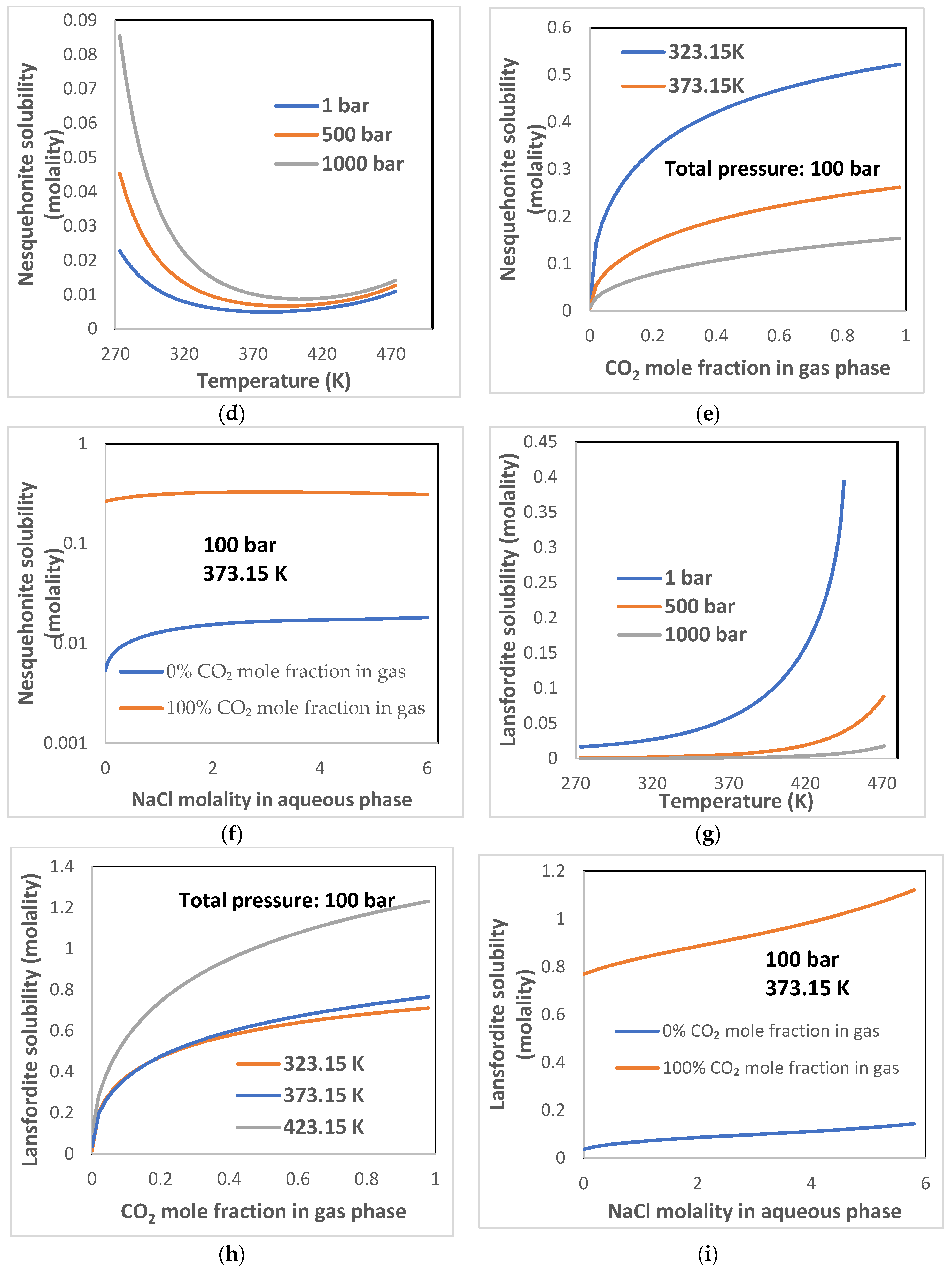
3.3.1. MgCO₃ Mineral Solubility

MgCO₃ mineral solubilities (i.e., lansfordite, magnesite, and nesquehonite) at various temperatures, pressures, and NaCl molalities are calculated by this model. Figure 6a shows the solubility of magnesite at temperature ranging between 0 and 200 °C, and pressure ranging between 1 and 1000 bar. Magnesite solubility decreases with temperature and increases with pressure. Figure 6b shows the magnesite solubility with CO₂ mole fraction at various temperatures and 100 bar. From the results, the presence of CO₂ in gas phase significantly enhances magnesite solubility in water. Figure 6c shows the magnesite solubility varying with NaCl molalities at 100 bar and various temperatures under conditions of gas free or 100% CO₂. The NaCl molality can enhance the dissolution of magnesite. With same temperature, pressure, and NaCl molality, when the solution is in equilibrium with CO₂, the magnesite solubility increase is significant.

Similar behavior of nesquehonite and lansfordite solubilities are observed from Figure 6d–i at various conditions except temperature effects. Nesquehonite solubility in water decreases with temperature at lower temperature range (about 0–120 °C) and increases with temperature at higher temperature range (about more than 120 °C, Figure 6d). Lansfordite solubility in water increases with temperature with the entire range from 0–200 °C (Figure 6g).

3.3.2. Solution Properties

With the new thermodynamic model of CO₂-H₂O-NaCl-MgCO₃ systems, the solution properties (such as pH, various species concentrations, distribution of carbonate species, etc.) can be calculated. Figure 7 shows the pH of solutions (saturated with CO₂) varying with pressure from 1 to 1000 bar at different temperatures under conditions of MgCO₃ saturated or free. NaCl molality is 4 molal for all the scenarios. From Figure 7, equilibrium with MgCO₃ minerals can significantly increase pH values of the solutions. The MgCO₃ minerals can be treated as “buffer minerals” for aqueous solutions.

From the previous sections, when CO₂ or carbonate minerals dissolved in water, it can be in the forms of CO₂^(aq), HCO₃⁻, CO₃²⁻, and MgCO₃^(aq). Figure 8 shows the various carbon species concentrations varying with pressure at 100 °C under conditions of MgCO₃ minerals saturated or free. At different conditions, most of the carbon in aqueous solution is in the form of CO₂^(aq), and HCO₃⁻ is secondary. When the solutions are in equilibrium with the MgCO₃ minerals, higher concentrations of different forms of carbon can be observed.

4. Conclusions

With regards to the importance of magnesium carbonate minerals to CO₂ geological storage projects, we developed a thermodynamic model of CO₂-H₂O-NaCl-MgCO₃ systems from 0–200 °C, 1–1000 bar, and halite up to high concentration. The model can calculate the phase equilibria and speciation including gas phase mole fractions, molality of aqueous species (such as CO₃²⁻, HCO₃⁻, Mg²⁺, Mg(OH)⁺, H⁺, OH⁻, CO₂^(aq), and MgCO₃^(aq)), pH, and dissolution and precipitation of MgCO₃ minerals.

To validate the model, we compared the model results with the current existing data in terms of CO₂ solubility in aqueous solutions, and MgCO₃ mineral solubilities. From the comparison, CO₂ solubility in NaCl solutions can be reproduced in a wide temperature, pressure, and salinity range with similar accuracy as the previous work [31,46]. The experimental solubility of nesquehonite, magnesite, and lansfordite in aqueous solutions with various temperature and CO₂ partial pressure can be reproduced by this model. The AAD% between model results and experimental data are calculated. From the results, most of the experimental data can be reproduced with AAD% less than 10%.

The model is used for the prediction of phase equilibria of CO₂-H₂O-NaCl-MgCO₃ systems with temperature from 0–200 °C, pressure from 1–1000 bar, and halite concentration up to 6 molal. From the results, the followings can be concluded.

(1)

Temperature usually decreases the mineral solubilities, and pressure usually increases the solubility. However, for nesquehonite, the solubility decreases with temperature when the temperature is less than about 100 °C and increases when the temperature is higher than 100 °C. For lansfordite, the solubility increases with temperature from 0–200 °C.

(2)

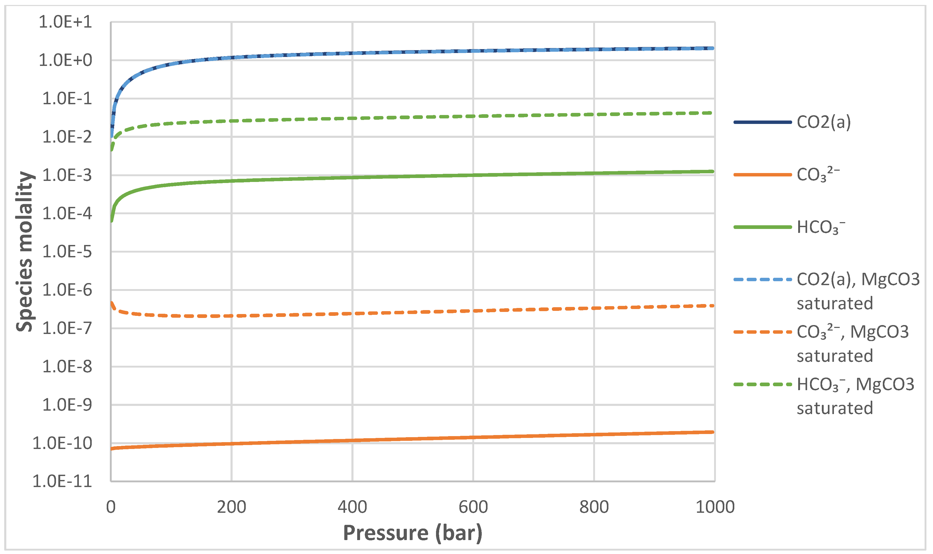
The presence of CO₂ in aqueous solution or gases phase will significantly enhance the dissolution of MgCO₃ minerals.

(3)

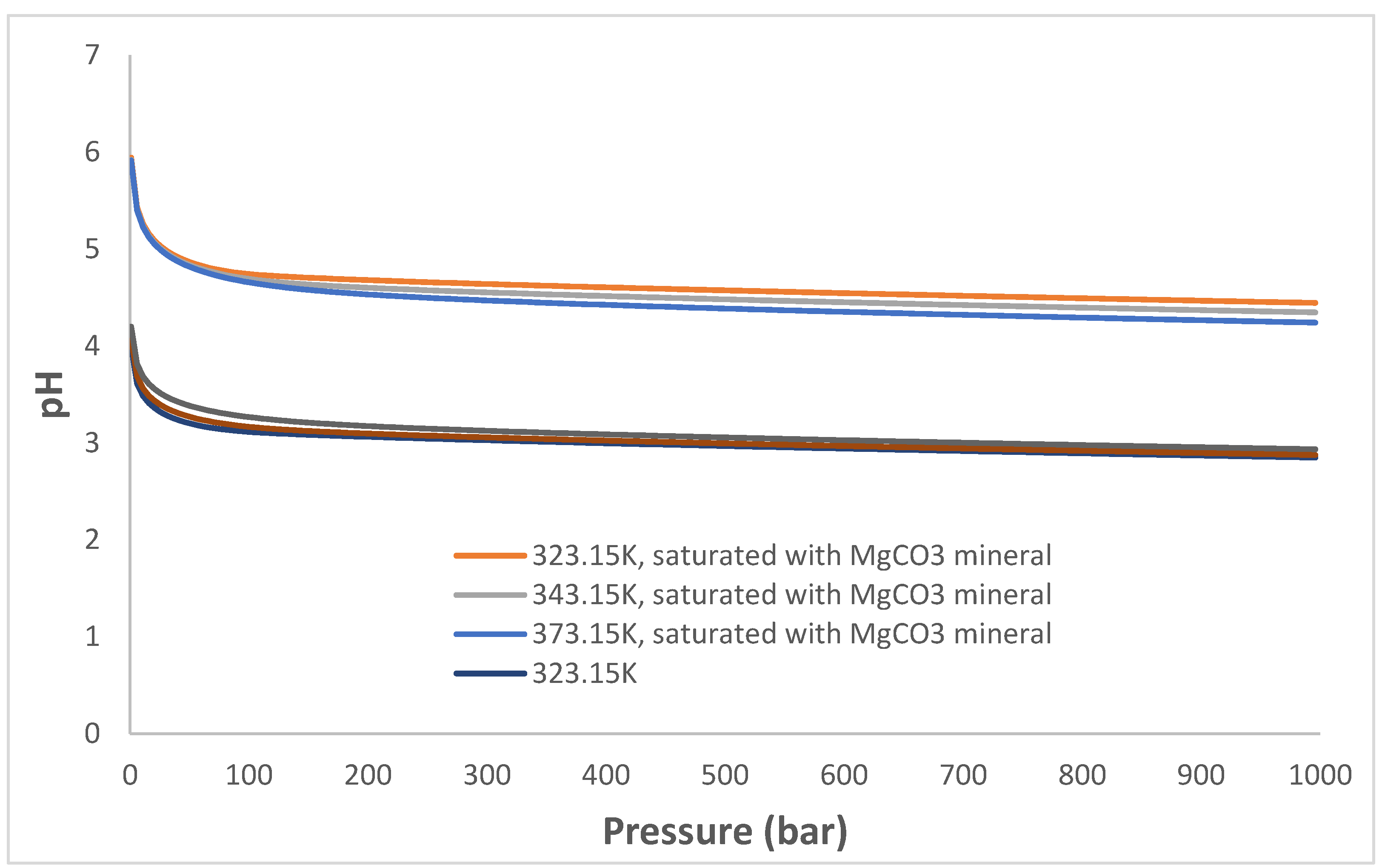
For CO₂ saturated solutions, the dissolution of MgCO₃ minerals will increase the pH of the solutions at different temperature and pressure conditions. MgCO₃ minerals can be treated as “buffer minerals”.

(4)

The influences of MgCO₃ minerals on CO₂ solubility are insignificant. However, the concentrations of carbon-bearing ions in the solutions are significantly increased by the dissolution of MgCO₃ minerals.

References

- Zhao, H.; Liao, X.; Chen, Y.; Zhao, X. Sensitivity analysis of CO2 sequestration in saline aquifers. Pet. Sci. 2010, 7, 372–378. [Google Scholar] [CrossRef]
- Li, J.; Ahmed, R.; Li, X. Thermodynamic modeling of CO2-N2-O2-Brine-Carbonates in conditions from surface to high temperature and pressure. Energies 2018, 11, 2627. [Google Scholar] [CrossRef]
- Bénézeth, P.S.; Saldi, G.D.; Dandurand, J.-L.; Schott, J. Experimental determination of the solubility product of magnesite at 50 to 200 °C. Chem. Geol. 2011, 286, 21–31. [Google Scholar] [CrossRef]
- Li, J.; Li, X. Analysis of u-tube sampling data based on modeling of CO2 injection into CH4 saturated aquifers. Greenh. Gases: Sci. Technol. 2015, 5, 152–168. [Google Scholar] [CrossRef]
- Wagner, R. Ueber die löslichkeit einiger erd-und metallcarbonate in kohlensäurehaltigem wasser. J. Anal. Chem. 1867, 6, 233–238. [Google Scholar] [CrossRef]
- Cameron, F.K.; Briggs, L.J. Equilibrium between carbonates and bicarbonates in aqueous solution. J. Phys. Chem. 1901, 5, 537–555. [Google Scholar] [CrossRef][Green Version]
- Wells, R.C. The solubility of magnesium carbonate in natural waters.2. J. Am. Chem. Soc. 1915, 37, 1704–1707. [Google Scholar] [CrossRef]
- Bär, O. Beitrag zum thema dolomitentstehung. Zentr. Mineral. Geol. Palaontol. Abt. A 1932, 1932, 46–62. [Google Scholar]
- Halla, F.; Chilingar, G.V.; Bissell, H.J. Thermodynamic studies on dolomite formation and their geologic implications: An interim report. Sedimentology 1962, 1, 296–303. [Google Scholar] [CrossRef]
- Berg, L.G.; Borisova, L.A. Solubility isotherms of the ternary systems Mg2+, Ca2+//CO32−, H2O, Na+, Ca2+//CO32−, H2O and Na+, Mg2+//CO32−, H2O at 25 °C and PCO2 = 1 atmosphere. Russ. J. Inorg. Chem. 1960, 5, 618–620. [Google Scholar]
- Christ, C.L.; Hostetler, P.B. Studies in the system MgO-SiO2-CO2-H2O (ii); the activity-product constant of magnesite. Am. J. Sci. 1970, 268, 439–453. [Google Scholar] [CrossRef]
- Cameron, F.K.; Seidell, A. The solubility of magnesium carbonate in aqueous solutions of certain electrolytes. J. Phys. Chem. 2002, 7, 578–590. [Google Scholar] [CrossRef][Green Version]
- Engel, M. Sur la solubilité des sels en présence des acides, des bases et de sels. Ann. Chim. Phys. 1889, 17, 349–369. [Google Scholar]
- Königsberger, E.; Königsberger, L.-C.; Gamsjäger, H. Low-temperature thermodynamic model for the system Na2CO3−MgCO3−CaCO3−H2O. Geochim. Cosmochim. Acta 1999, 63, 3105–3119. [Google Scholar] [CrossRef]
- Kline, W.D. The solubility of magnesium carbonate (nesquehonite) in water at 25 °C and pressures of carbon dioxide up to one atmosphere1. J. Am. Chem. Soc. 1929, 51, 2093–2097. [Google Scholar] [CrossRef]
- Mitchell, A.E. Ccxii.—studies on the dolomite system.—Part ii. J. Chem. Soc. Trans. 1923, 123, 1887–1904. [Google Scholar] [CrossRef]
- Haehnel, O. Über die löslichkeit des magnesiumcarbonats in kohlensäurehaltigem wasser unter höheren kohlendioxyddrucken und über die eigenschaften solcher magnesiumbicarbonatlösungen. J. für Prakt. Chem. 1924, 108, 61–74. [Google Scholar] [CrossRef]
- Yanat’eva, O.K. Solubility of the system Ca, Mg-CO3, SO4-H2O at 25 °C and PCO2 of 0.0012 atm. Zh. Neorgan. Khim. 1957, 2, 2183–2187. [Google Scholar]
- Takahashi, G. Investigation on the synthesis of potassium carbonate by Mr. Engel. Bull. Imp. Hyg. Lab. (Tokyo) 1927, 29, 165–262. [Google Scholar]
- Ponizovskii, A.M.; Vladimirova, N.M.; Gordon-Yanovskii, F.A. The solubility relation in the system Na, Mg-Cl, HCO3-H2O at 0°C with carbon dioxide at 4 and 10 kg/cm2. Russ. J. Inorg. Chem. 1960, 5, 1250–1252. [Google Scholar]
- Yanat’eva, O.K.; Rassonskaya, I.S. Metastable equilibria and solid phases in the CaCO3-MgCO3-H2O system. Russ. J. Inorg. Chem. 1961, 6, 730–733. [Google Scholar]
- Harvie, C.E.; Weare, J.H. The prediction of mineral solubilities in natural waters: The Na-K-Mg-Ca-Cl-SO4-H2O system from zero to high concentration at 25 °C. Geochim. Cosmochim. Acta 1980, 44, 981–997. [Google Scholar] [CrossRef]
- Harvie, C.E.; Møller, N.; Weare, J.H. The prediction of mineral solubilities in natural waters: The Na-K-Mg-Ca-H-Cl-SO4-OH-HCO3-CO3-CO2-H2O system to high ionic strengths at 25 °C. Geochim. Cosmochim. Acta 1984, 48, 723–751. [Google Scholar] [CrossRef]
- Pitzer, K.S. Thermodynamics of electrolytes. I. Theoretical basis and general equations. J. Phys. Chem. 1973, 77, 268–277. [Google Scholar] [CrossRef]
- Pitzer, K.S.; Mayorga, G. Thermodynamics of electrolytes. II. Activity and osmotic coefficients for strong electrolytes with one or both ions univalent. J. Phys. Chem. 1973, 77, 2300–2308. [Google Scholar] [CrossRef]
- Pitzer, K.S.; Kim, J.J. Thermodynamics of electrolytes. IV. Activity and osmotic coefficients for mixed electrolytes. J. Am. Chem. Soc. 1974, 96, 5701–5707. [Google Scholar] [CrossRef]
- Pitzer, K.S. Thermodynamic properties of aqueous sodium chloride solutions. J. Phys. Chem. Ref. Data 1984, 13, 1–102. [Google Scholar] [CrossRef]
- Møller, N. The prediction of mineral solubilities in natural waters: A chemical equilibrium model for the Na-Ca-Cl-SO4-H2O system, to high temperature and concentration. Geochim. Cosmochim. Acta 1988, 52, 821–837. [Google Scholar] [CrossRef]
- Greenberg, J.P.; Møller, N. The prediction of mineral solubilities in natural waters: A chemical equilibrium model for the Na-K-Ca-Cl-SO4-H2O system to high concentration from 0 to 250 °C. Geochim. Cosmochim. Acta 1989, 53, 2503–2518. [Google Scholar] [CrossRef]
- Christov, C.; Moller, N. Chemical equilibrium model of solution behavior and solubility in the H-Na-K-OH-Cl-HSO4-SO4-H2O system to high concentration and temperature.11 associate editor: Wesolowski. D. J. Geochim. Cosmochim. Acta 2004, 68, 1309–1331. [Google Scholar] [CrossRef]
- Duan, Z.; Sun, R. An improved model calculating CO2 solubility in pure water and aqueous NaCl solutions from 273 to 533 K and from 0 to 2000 bar. Chem. Geol. 2003, 193, 257–271. [Google Scholar] [CrossRef]
- Duan, Z.; Li, D. Coupled phase and aqueous species equilibrium of the H2O–CO2–NaCl–CaCO3 system from 0 to 250 °C, 1 to 1000 bar with NaCl concentrations up to saturation of halite. Geochim. Cosmochim. Acta 2008, 72, 5128–5145. [Google Scholar] [CrossRef]
- Li, D.; Duan, Z. The speciation equilibrium coupling with phase equilibrium in the H2O–CO2–NaCl system from 0 to 250 °C, from 0 to 1000 bar, and from 0 to 5 molality of NaCl. Chem. Geol. 2007, 244, 730–751. [Google Scholar] [CrossRef]
- Li, J.; Duan, Z. A thermodynamic model for the prediction of phase equilibria and speciation in the H2O–CO2–NaCl–CaCO3–CaSO4 system from 0 to 250 °C, 1 to 1000 bar with NaCl concentrations up to halite saturation. Geochim. Cosmochim. Acta 2011, 75, 4351–4376. [Google Scholar] [CrossRef]
- Parkhurst, D.L.; Appelo, C.A.J. User’s guide to PHREEQC (Version 2)—A computer program for speciation, batch-reaction, one-dimensional transport, and inverse geochemical calculations. Water-Resour. Investig. Rep. 1999, 99, 312. [Google Scholar]
- Xu, T.; Spycher, N.; Sonnethal, E.; Zhang, G.; Zheng, L.; Pruess, K. TOUGHREACT Version 2.0: A simulator for subsurface reactive transport under non-isothermal multiphase flow conditions. Comput. Geosci. 2011, 37, 763–774. [Google Scholar] [CrossRef]
- Su, D.; Mayer, K.U.; MacQuarrie, K.T. Parallelization of MIN3P-THCm: A high performance computational framework for subsurface flow and reactive transport simulation. Environ. Model. Softw. 2017, 95, 271–289. [Google Scholar] [CrossRef]
- Wolery, T.J. EQ3/6 A Software Package for Geochemical Modeling (Version 05). Report Number: LLNL-CODE-638958. Available online: https://www.osti.gov//servlets/purl/1231666 (accessed on 28 November 2019).
- Zhu, C.; Burden, D.S. Mineralogical compositions of aquifer matrix as necessary initial conditions in reactive contaminant transport models. J. Contam. Hydrol. 2001, 51, 145–161. [Google Scholar] [CrossRef]
- Dobson, P.; Salah, S.; Spycher, N.; Sonnenthal, E.L. Simulation of Water-Rock interaction in the Yellowstone Geothermal system using TOUGHREACT. Geochermics 2004, 33, 493–502. [Google Scholar] [CrossRef]
- Zhang, W.; Shi, W.; Li, J.; Deng, G.; Chang, Y.; Li, Z. Application of geochemical code EQ3/6 to leaching technique of hard rock uranium deposit. J. East. China Geol. Inst. 1997, 20, 362–367. [Google Scholar]
- Computer Modeling Group (CMG), User Technical Manual; Computer Modelling Group Ltd.: Calgary, Canada, 2016.
- Wei, L. Sequential Coupling of Geochemical Reactions With Reservoir Simulations for Waterflood and EOR Studies. SPE J. 2012, 17, 469–484. [Google Scholar] [CrossRef]
- Adegbite, J.O.; Al-Shalabi, E.W.; Ghosh, B. Modeling the Effect of Engineered Water Injection on Oil Recovery from Carbonate Cores. In Proceedings of the SPE International Conference on Oilfield Chemistry, Montgomery, TX, USA, 3–5 April 2017. [Google Scholar] [CrossRef]
- Li, X.; Wei, L.; Zhang, H. Improving Reactive Transport Modeling Predictivity for ASP Flooding Simulations. In Proceedings of the SPE EOR Conference at Oil and Gas West Asia, Muscat, Oman, 21–23 March 2016; pp. 1–20. [Google Scholar] [CrossRef]
- Li, J.; Wei, L.; Li, X. An improved cubic model for the mutual solubilities of CO2–CH4–H2S–brine systems to high temperature, pressure and salinity. Appl. Geochem. 2015, 54, 1–12. [Google Scholar] [CrossRef]
- Appelo, C.A.J.; Parkhurst, D.L.; Post, V.E.A. Equations for calculating hydrogeochemical reactions of minerals and gases such as CO2 at high pressures and temperatures. Geochim. Cosmochim. Acta 2014, 125, 49–67. [Google Scholar] [CrossRef]
- Helgeson, H.C.; Kirkham, D.H.; Flowers, G.C. Theoretical prediction of the thermodynamic behavior of aqueous electrolytes at high pressures and temperatures: Calculation of activity coefficients, osmotic coefficients, and apparent molal and standard and relative partial modal properties to 600 °C and 5 Kb. Am. J. Sci. 1981, 281, 1249–1516. [Google Scholar] [CrossRef]
- Duan, Z.; Sun, R.; Zhu, C.; Chou, I.M. An improved model for the calculation of CO2 solubility in aqueous solutions containing Na+, K+, Ca2+, Mg2+, Cl−, and SO42−. Mar. Chem. 2006, 98, 131–139. [Google Scholar] [CrossRef]
- Peng, D.-Y.; Robinson, D.B. A new two-constant equation of state. Ind. Eng. Chem. Fundam. 1976, 15, 59–64. [Google Scholar] [CrossRef]
- Michelsen, M.L.; Mollerup, J.M. Thermodynamic models: Fundamentals & Computational Aspects, 2nd ed.; TIE-LINE Publications: Herning, Denmark, 2007. [Google Scholar]
- Visscher, A.D.; Vanderdeelen, J.; Königsberger, E.; Churagulov, B.R.; Ichikuni, M.; Tsurumi, M. Iupac-nist solubility data series. 95. Alkaline earth carbonates in aqueous systems. Part 1. Introduction, be and mg. J. Phys. Chem. Ref. Data. 2012, 41, 013105. [Google Scholar] [CrossRef]