Dual Solutions and Stability Analysis of Micropolar Nanofluid Flow with Slip Effect on Stretching/Shrinking Surfaces

Abstract

The purpose of the present paper is to investigate the micropolar nanofluid flow on permeable stretching and shrinking surfaces with the velocity, thermal and concentration slip effects. Furthermore, the thermal radiation effect has also been considered. Boundary layer momentum, angular velocity, heat and mass transfer equations are converted to non-linear ordinary differential equations (ODEs). Then, the obtained ODEs are solved by applying the shooting method and in the results, the dual solutions are obtained in the certain ranges of pertinent parameters in both cases of shrinking and stretching surfaces. Due to the presence of the dual solutions, stability analysis is done and it was found that the first solution is stable and physically feasible. The results are also compared with previously published literature and found to be in excellent agreement. Moreover, the obtained results reveal the angular velocity increases in the first solution when the value of micropolar parameter increases. The velocity of nanofluid flow decreases in the first solution as the velocity slip parameter increases, whereas the temperature profiles increase in both solutions when thermal radiation, Brownian motion and the thermophoresis parameters are increased. Concentration profile increases by increasing $N_t$ and decreases by increasing $N_b$.

1. Introduction

The boundary flow and heat transfer phenomena of all types of fluids have remained of great interest for many researchers, especially for purpose of the practical implementation. Originally, fluids are classified into Newtonian and non-Newtonian fluids. There are many industrial applications of non-Newtonian fluids, such as drilling mud, polycrystal melts, oils, certain paints, volcanic lava, cosmetic product, fluid suspensions, molten polymers and food product, etc. There are many mathematical models for various constitutive equations that deal with flow phenomena with different parameters. Among such models, the micropolar fluid model is one of the non-Newtonian models introduced by Eringen [1]. This model deals with the flow of the micropolar fluids, whereas some examples of the micropolar fluids are liquid crystals with rigid molecules, suspensions or colloidal solutions, some biological fluids, exocytic lubricants and the blood of the animals, etc. In many industries, fluids are used for heat transport purposes, but common fluids are weak source of the heat transport. So, with development of nanotechnology, in the field of fluid mechanics, Choi and Eastman [2] introduced a new kind of modern fluid that could suspend the solid nanoparticles into common base fluids, later named as nanofluid. Nanofluids possess high thermal conductivity as compared to all concerned host fluids. Nanofluids is a sub-class of the modern rapidly growing field of nanoscience and technology.

Several practical problems have been discussed by many researchers in order to enhance thermal conductivity for the last many years. There are two well-known models that support transport phenomena of nanofluids, which are the Tiwari and Das model [3] and Buongiorno’s model [4]. It should be noted that Buongiorno’s model is considered a two-phase non-homogeneous model in which the slip velocity of the base fluid and nanoparticles are not equal to zero. This model contains seven slip parameters, including diffusiophoresis, inertia, fluid drainage, gravity, Brownian motion, Magnus and thermophoresis [5]. On the other hand, the Tiwari-Das model is one of the single-phase (homogeneous) models in which the thermophysical characteristics of the base fluid are improved with the impact of nanoparticles allied with viscosity and thermal conductivity. Many researchers considered these two models to study all types of nanofluids as well as micropolar nanofluids, such as Hsiao [6], Lund et al. [7,8], Hashemi et al. [9], Hussain et al. [10], Dero et al. [11,12,13], Alarifi et al. [14] Pourfattah et al. [15], Alsarraf et al. [16], Jafarimoghaddam et al. [17,18], and Pal and Mandal [19]. Further work on nanofluid is referenced in [20,21,22]. In the present research, Buongiorno’s model is considered in order to develop the mathematical model for boundary layer micropolar nanofluid flow with slip parameters and radiation effect. It is observed that a little attention is given to this model for the case of existing multiple solutions in flow of the micropolar nanofluid.

The velocity, temperature and concentration slip factors may exist in case of rising the relative difference among velocity, temperature and the concentration entities. Awais et al. [23] studied the different slip conditions on a stretching sheet. They stated that if the temperature in the fluid flow is controlled by the thermal slip parameter then there is the possibility the concentration may also be controlled through transport phenomena of mass transfer. Das [24] examined the velocity slip on micropolar viscous fluid and found the increasing value of the velocity slip parameter will decrease the velocity as well as the thickness of the boundary layer. Ramya et al. [25] considered the nanofluid with thermal and velocity slip parameters. Some studies of micropolar nanofluid with different slip conditions can be found in [26,27,28,29].

It has been observed in previous literature that the work on the non-Newtonian nanofluid flow is very limited. Therefore, in present research work, a non-Newtonian micropolar nanofluid is considered by using a two-phase model. There study of Hayat et al. [30] examined the two-dimensional incompressible micropolar nanofluid flow over a linearly stretching/shrinking sheet with velocity, thermal and concentration slip effects. To the best of the author’s knowledge, the multiple similarity solutions with stability analysis of micropolar nanofluid flow on a permeable stretching and shrinking surface along the velocity, thermal and the concentration slip effects have not been studied by any other researcher in the past years. Thus, the purpose of the present work is to determine the multiple similarity solutions with stability analysis of the micropolar nanofluid flow with thermal radiation and slip effects. Buongiorno’s model is used due to its novelty of thermophoresis and Brownian motion of small particles. Furthermore, numerical solutions have been obtained by applying the shooting technique with shootlib function in the Maple software. There has been stability analysis performed in order to determine the stable solution with the help of BVP4C solver. The graphical results of different applied parameters are illustrated in the discussions. Furthermore, the physical behaviors of the skin friction coefficient, and the local Nusselt and Sherwood number are discussed. The main focus of this paper is to determine the multiple similarity solutions with stability analysis of micropolar boundary layer nanofluid and to understand the behavior of different parameters in the flow and heat transfer characteristics. It is expected that the present study will help those researchers interested in multiple similarity solutions with stability analysis in micropolar nanofluid flows.

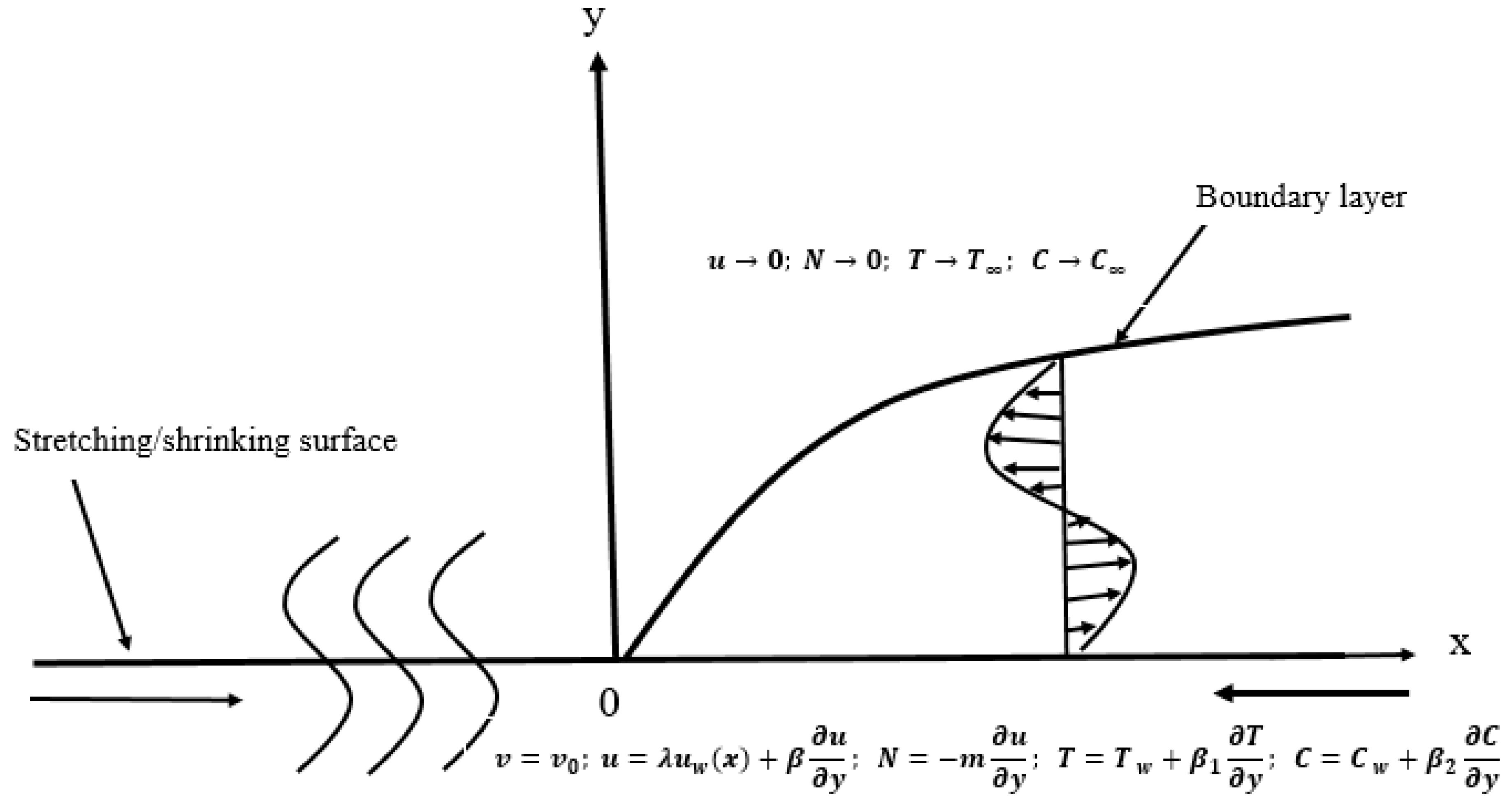
2. Flow Analysis

Two-dimensional incompressible micropolar nanofluid flow through a linearly shrinking and stretching surfaces with velocity, thermal and concentration slip effects are shown in Figure 1 Furthermore, the effects of Brownian motion and the thermophoresis have been considered in Newtonian heat and concentration equations with thermal radiation effect. By using the above-mentioned assumptions as well as boundary layer approximations, the system of governing equations of micropolar boundary layer nanofluid flow will be written as:

$$\frac{\partial u}{\partial x}+\frac{\partial v}{\partial y}=0$$

(1)

$$u \frac{\partial u}{\partial x} + v \frac{\partial u}{\partial y}=\left(\vartheta +\frac{\kappa }{\rho }\right)\frac{{\partial }^{2}u}{\partial y^2}+\frac{\kappa }{\rho }\frac{\partial N}{\partial y}$$

(2)

$$u\frac{\partial N}{\partial x}+v\frac{\partial N}{\partial y}=\frac{1}{\rho j}\left[\gamma \frac{{\partial }^{2}N}{\partial y^2}-\kappa \left(2N+\frac{\partial u}{\partial y}\right)\right]$$

(3)

$$u \frac{\partial T}{\partial x} + v \frac{\partial T}{\partial y} =\left(\alpha +\frac{16{\sigma }^{*}{T}_{\infty }^3}{3K^{*}\rho c_p} \right) \frac{{\partial }^{2}T}{\partial y^2} + {\tau }_w \left[D_B \frac{\partial C}{\partial y} \frac{\partial T}{\partial y} + \frac{D_T}{T_{\infty }} {\left(\frac{\partial T}{\partial y}\right)}^2\right]$$

(4)

$$u \frac{\partial C}{\partial x} + v \frac{\partial C}{\partial y}=D_B \frac{{\partial }^{2}C}{\partial y^2} + \frac{D_T}{T_{\infty }} \frac{{\partial }^{2}T}{\partial y^2}$$

(5)

Subject to boundary conditions

$$\begin{gathered} v=v_0; u=\lambda u_w\left(x\right)+\beta \frac{\partial u}{\partial y}; N=-m\frac{\partial u}{\partial y}; T=T_{ w}+{\beta }_1\frac{\partial T}{\partial y}; C=C_{ w}+{\beta }_2\frac{\partial C}{\partial y} at y=0 \\ u\to 0; N\to 0; T\to T_{\infty }; C\to C_{\infty } as y\to \infty \end{gathered}$$

(6)

Where $u$ and $v$ represent velocity components in the directions of the $x$-axis and $y$-axis, respectively. While $\vartheta$, $\rho$, $\kappa ,$ $N$,$\gamma$ and $j$ are kinematic energy, fluid density, vortex viscosity, angular velocity, spin gradient viscosity and micro-inertia density, respectively. Furthermore, $T$, $\alpha$, $K^{*}$, ${\sigma }^{*}$, ${\tau }_w$, $D_B$, $D_T$, $T_{\infty }$ and $C$ are temperature, thermal diffusivity of nanofluid, mean absorption coefficient, Stefan–Boltzmann constant, ratio of effective heat capacity of nanoparticles of solid material to the heat capacity of fluid, thermophoretic diffusion coefficient, coefficient of Brownian diffusion, free stream temperature and concentration field, respectively. $v_0$ is mass flux velocity, $u_w\left(x\right)=ax$ is shrinking/stretching velocity of surface and $\lambda$ is shrinking/stretching parameter where $\lambda <0$ indicates shrinking surface while $\lambda >0$ indicates stretching surface and $\beta , {\beta }_1 and {\beta }_2$ are the velocity, heat transfer and the concentration slip parameters, respectively.

The following similarity variables are applied to determine the similarity solutions of the problem.

$$\begin{gathered} \eta =y\sqrt{\frac{a}{\vartheta }},u=ax{f}^{\prime }\left(\eta \right),v=-\sqrt{a\vartheta }f\left(\eta \right),N=\sqrt{\frac{a}{\vartheta }}axg\left(\eta \right),\theta \left(\eta \right)=\frac{\left(T-T_{\infty }\right)}{\left(T_w- T_{\infty }\right)}, \\ \varnothing \left(\eta \right)=\frac{\left(C-C_{\infty }\right)}{\left(C_w- C_{\infty }\right)}, \end{gathered}$$

(7)

By using similarity transformations (7) in Equations (1)–(5), the following ODEs are obtained,

$$\left(1+K\right)f^{‴}+f{f}^{″}-f^{\prime 2}+K{g}^{\prime }=0$$

(8)

$$\left(1+\frac{K}{2}\right) g^{″}+f{g}^{\prime }-g{f}^{\prime }-2Kg-K{f}^{″}=0$$

(9)

$$\frac{1}{Pr}\left(1+\frac{4}{3}Rd\right){\theta }^{″}+f{\theta }^{\prime }+N_b{\varnothing }^{\prime }{\theta }^{\prime }+N_t{\left({\theta }^{\prime }\right)}^2=0$$

(10)

$$\frac{1}{Sc}{\varnothing }^{″}+f{\varnothing }^{\prime }+\frac{1}{Sc}\frac{N_t}{N_b}{\theta }^{″}=0$$

(11)

subject to boundary conditions

$$\begin{gathered} f\left(0\right)=f_w, f^{\prime }\left(0\right)=\lambda +\delta f^{″}\left(0\right), g\left(0\right)=-m{f}^{″}\left(0\right), \theta \left(0\right)=1+{\delta }_T\theta \prime \left(0\right), \varnothing \left(0\right)=1+{\delta }_C{\varnothing }^{\prime }\left(0\right) \\ {f}^{\prime }\left(\eta \right)\to 0, g\left(\eta \right)\to 0, \theta \left(\eta \right)\to 0, \varnothing \left(\eta \right)\to 0 \mathrm{as} \eta \to \infty \end{gathered}$$

(12)

where, prime indicates differentiation with respect to the variable $\eta$, $K=\frac{\kappa }{\mu }$ is the micropolar material parameter, $Pr=\frac{\vartheta }{\alpha }$ is a Prandtl number, $Rd=\frac{4\sigma T_{\infty }^3}{K^{*}k}$ is thermal radiation parameter, $N_b=\frac{{\tau }_w{D}_B\left(C_w-C_{\infty }\right)}{\vartheta }$ is a Brownian motion parameter, $N_t=\frac{{\tau }_w{D}_T\left(T_w-T_{\infty }\right)}{\vartheta T_{\infty }}$ is a thermophoresis parameter and $Sc= \frac{\vartheta }{D_B}$ is the Schmidt number. Moreover, $f_w=-\frac{v_0}{\sqrt{a\vartheta }}$ is the suction parameter ($f_w>0$), $\delta =\beta \sqrt{\frac{a}{\vartheta }}$ is a velocity slip, ${\delta }_T={\beta }_1\sqrt{\frac{a}{\vartheta }}$ is a thermal slip and ${\delta }_C={\beta }_2\sqrt{\frac{a}{\vartheta }}$ is concentration slip parameters. It should be noted that the values of $m=0$ show that the microelements are closed to surface with a strong concentration, which means the particles are not rotatable. In the same manner, $m=0.5$ shows that the concentration is week due to vanishing of the anti-symmetric part of the stress tensor. In addition, $m=1$ specifies the turbulent boundary layer flow model of Ramzan et al. [31].

Quantities of the physical interests are the coefficient of the skin friction $C_f$, local Nusselt number $N_u$ and Sherwood number $S_h$ that are stated as,

$$\begin{gathered} C_f=\frac{{\left[\left(\mu +\kappa \right)\frac{\partial u}{\partial y}+\kappa N\right]}_{y=0}}{\rho u_w^2}, N_u=\frac{-x{\left[\left(\frac{16{\sigma }^{*}{T}_{\infty }^3}{3K^{*}}+k\right)\frac{\partial T}{\partial y}\right]}_{y=0}}{\left(T_w- T_{\infty }\right)}, \\ {S}_h=\frac{-x{\left(\frac{\partial C}{\partial y}\right)}_{y=0}}{\left(C_w- C_{\infty }\right)} \end{gathered}$$

(13)

Using Equation (7) in (13), it is obtained

$$\begin{gathered} C_f{\left(R{e}_x\right)}^{\frac{1}{2}}=\left(1+\left(1-m\right)K\right)f^{″}\left(0\right), \\ {N}_u{\left(R{e}_x\right)}^{-\frac{1}{2}}=-\left(1+\frac{4}{3}Rd\right){\theta }^{\prime }\left(0\right), \\ {S}_h{\left(R{e}_x\right)}^{-\frac{1}{2}}=-{\varnothing }^{\prime }\left(0\right) \end{gathered}$$

(14)

where $R{e}_x=a{x}^2/\vartheta$ is a local Reynolds number.

3. Stability Analysis

The numerical computation of the Equations (8)–(11) with boundary conditions (12) shows the occurrence of the dual solutions. Therefore, it is necessary to perform the stability analysis to find the stable and physically feasible solution. For stability of solution, the first step is to convert governing Equations (2)–(5) into unsteady form by introducing a new time dependent variable $\tau$ as mentioned by [32,33,34].

$$\frac{\partial u}{\partial t} + u \frac{\partial u}{\partial x} + v \frac{\partial u}{\partial y}=\left(\vartheta +\frac{\kappa }{\rho }\right)\frac{{\partial }^{2}u}{\partial y^2}+\frac{\kappa }{\rho }\frac{\partial N}{\partial y}$$

(15)

$$\frac{\partial N}{\partial t}+u\frac{\partial N}{\partial x}+v\frac{\partial N}{\partial y}=\frac{1}{\rho j}\left[\gamma \frac{{\partial }^{2}N}{\partial y^2}-\kappa \left(2N+\frac{\partial u}{\partial y}\right)\right]$$

(16)

$$\frac{\partial T}{\partial t}+u \frac{\partial T}{\partial x} + v \frac{\partial T}{\partial y} =\left(\alpha +\frac{16{\sigma }^{*}{T}_{\infty }^3}{3K^{*}\rho c_p} \right) \frac{{\partial }^{2}T}{\partial y^2} + {\tau }_w \left[D_B \frac{\partial C}{\partial y} \frac{\partial T}{\partial y} + \frac{D_T}{T_{\infty }} {\left(\frac{\partial T}{\partial y}\right)}^2\right]$$

(17)

$$\frac{\partial C}{\partial t}+ u \frac{\partial C}{\partial x} + v \frac{\partial C}{\partial y}=D_B \frac{{\partial }^{2}C}{\partial y^2} + \frac{D_T}{T_{\infty }} \frac{{\partial }^{2}T}{\partial y^2}$$

(18)

Now, the new similarity variables have been introduced as follows

$$\begin{gathered} \eta =y\sqrt{\frac{a}{\vartheta }},\tau =at, u=ax\frac{\partial f\left(\eta , \tau \right)}{\partial \eta },v=-\sqrt{a\vartheta }f\left(\eta , \tau \right),N=\sqrt{\frac{a}{\vartheta }}axg\left(\eta , \tau \right), \\ \theta \left(\eta ,, \tau \right)=\frac{\left(T-T_{\infty }\right)}{\left(T_w- T_{\infty }\right)}, \varnothing \left(\eta , \tau \right)=\frac{\left(C-C_{\infty }\right)}{\left(C_w- C_{\infty }\right)}, \end{gathered}$$

(19)

By using Equation (19) in Equations (15)–(18), it is obtained

$$\left(1+K\right)\frac{{\partial }^{3}f}{\partial {\eta }^3}+f\frac{{\partial }^{2}f}{\partial {\eta }^2}-{\left(\frac{\partial f}{\partial \eta }\right)}^2+K\frac{\partial g}{\partial \eta }-\frac{{\partial }^{2}f}{\partial \tau \partial \eta }=0$$

(20)

$$\left(1+\frac{K}{2}\right) \frac{{\partial }^{2}g}{\partial {\eta }^2}+f\frac{\partial g}{\partial \eta }-g\frac{\partial f}{\partial \eta }-Kg-K\frac{{\partial }^{2}f}{\partial {\eta }^2}-\frac{\partial g}{\partial \tau }=0$$

(21)

$$\frac{1}{Pr}\left(1+\frac{4}{3}Rd\right)\frac{{\partial }^2\theta }{\partial {\eta }^2}+f\frac{\partial \theta }{\partial \eta }+N_b\frac{\partial \varnothing }{\partial \eta }\frac{\partial \theta }{\partial \eta }+N_t{\left(\frac{\partial \theta }{\partial \eta }\right)}^2-\frac{\partial \theta }{\partial \tau }=0$$

(22)

$$\frac{{\partial }^2\varnothing }{\partial {\eta }^2}+Sc.f\frac{\partial \varnothing }{\partial \eta }+\frac{N_t}{N_b}\frac{{\partial }^2\theta }{\partial {\eta }^2}-\frac{\partial \varnothing }{\partial \tau }=0$$

(23)

Subjected to boundary conditions

$$\begin{array}{c}f\left(0,\tau \right)=S;\frac{\partial f\left(0,\tau \right)}{\partial \eta }=\lambda +\delta \frac{{\partial }^{2}f\left(0,\tau \right)}{\partial {\eta }^2};g\left(0,\tau \right)=-m\frac{{\partial }^{2}f\left(0,\tau \right)}{\partial {\eta }^2};\theta \left(0,\tau \right)\\ =1+{\delta }_T\frac{\partial \theta \left(0,\tau \right)}{\partial \eta };\varnothing \left(0,\tau \right)=1+{\delta }_C\frac{\partial \varnothing \left(0,\tau \right)}{\partial \eta }\\ \frac{\partial f\left(\eta , \tau \right)}{\partial \eta }\to 0; g\left(\eta ,\tau \right)\to 0; \theta \left(\eta ,\tau \right)\to 0;\varnothing \left(\eta ,\tau \right)\to 0;as \eta \to \infty \end{array}$$

(24)

Now, there has been perturbed the basic solutions $f\left(\eta \right)=f_0\left(\eta \right)$, $g\left(\eta \right)=g_0\left(\eta \right)$, $\theta \left(\eta \right)={\theta }_0\left(\eta \right)$ and $\varnothing \left(\eta \right)={\varnothing }_0\left(\eta \right)$ with disturbances as

$$\begin{gathered} f\left(\eta ,\tau \right)=f_0\left(\eta \right)+e^{-\epsilon \tau }F\left(\eta \right) \\ g\left(\eta ,\tau \right)=g_0\left(\eta \right)+e^{-\epsilon \tau }G\left(\eta \right) \\ \theta \left(\eta ,\tau \right)={\theta }_0\left(\eta \right)+e^{-\epsilon \tau }H\left(\eta \right) \\ \varnothing \left(\eta ,\tau \right)={\varnothing }_0\left(\eta \right)+e^{-\epsilon \tau }S\left(\eta \right) \end{gathered}$$

(25)

where smallest eigenvalue is $\epsilon$ and $F\left(\eta \right)$, $G\left(\eta \right)$, $H\left(\eta \right)$ and $S\left(\eta \right)$ are small relative to $f_0\left(\eta \right)$, $g_0\left(\eta \right)$, ${\theta }_0\left(\eta \right)$ and ${\varnothing }_0\left(\eta \right)$ respectively. In the last one, the following system of linearized eigenvalue problems was obtained:

$$\left(1+K\right)F_0^{‴}+f_0{F}_0^{″}+F_0{f}_0^{″}-2f_0^{\prime }{F}_0^{\prime }+K{G}_0^{\prime }+\epsilon F_0^{\prime }=0$$

(26)

$$\left(1+\frac{K}{2}\right)G_0^{″}+f_0{G}_0^{\prime }+F_0{g}_0^{\prime }-g_0{F}_0^{\prime }-g_0{F}_0^{\prime }-2K{G}_0-K{F}_0^{″}+\epsilon G_0=0$$

(27)

$$\frac{1}{Pr}\left(1+\frac{4}{3}Rd\right)H_0^{″}+f_0{H}_0^{\prime }+F_0{\theta }_0^{\prime }+N_b{\varnothing }_0^{\prime }{H}_0^{\prime }+N_b{S}_0^{\prime }{\theta }_0^{\prime }+2N_t{\theta }_0^{\prime }{H}_0^{\prime }+\epsilon H_0=0$$

(28)

$$S_0^{″}+Sc\left(f_0{\varnothing }_0^{\prime }+F_0{S}_0^{\prime }\right)+\frac{N_t}{N_b}{H}_0^{″}+Sc.\epsilon S_0=0$$

(29)

with boundary conditions

$$\begin{gathered} F_0\left(0\right)=0, F_0^{\prime }\left(0\right)=\delta F_0^{″}\left(0\right), G_0\left(0\right)=-m{F}_0^{″}\left(0\right), H_0\left(0\right)={\delta }_T{H}_0^{\prime }\left(0\right), S_0\left(0\right)={\delta }_C{S}_0^{\prime }\left(0\right) \\ {F}_0^{\prime }\left(\eta \right)\to 0, G_0\left(\eta \right)\to 0, H_0\left(\eta \right)\to 0, S_0\left(\eta \right)\to 0 as \eta \to \infty \end{gathered}$$

(30)

The above-mentioned linearized Equations (26)–(29) with boundary conditions (30) are solved by using BVP4c solver function in MATLAB software and found values of smallest eigenvalue $\epsilon$. In order to find the smallest eigenvalues, there is to be relaxed one of the boundary conditions into initial condition as recommended by Harris et al. [35] and Ali et al. [36]. In this particular problem, there is relaxed the $G_0\left(\eta \right)\to 0$ as $\eta \to \infty$ into $G_0^{\prime }\left(0\right)=1$. It should be noted that negative smallest eigenvalues indicate the initial growth of disturbance, henceforth the solution of fluid flow becomes unstable. Whereas, if smallest eigenvalue value is positive, that flow of fluid is stable and physically realizable.

4. Result and Discussion

The governing equations of boundary layer micropolar nanofluid flow [8,9,10,11] subject to boundary conditions (12) are solved by shooting method with help of Maple software. The results of the momentum, angular velocity, temperature and concentration profiles are demonstrated graphically for different values of various physical parameters such as micropolar material, Brownian motion, thermal radiation, thermophoresis, and slip parameters. The obtained results are compared to those obtained by Hayat et al. [30] using homotopy analysis method (HAM) for the values of skin friction coefficients presented in

Table 1. Comparative results for surface drag force $(C_f{\left(R{e}_x\right)}^{\frac{1}{2}})$ for various values of $m=0, 0.5$ for the micropolar fluid with Hayat et al for the various values of $K$ at $\lambda =1$ and $f_w=0$. Reproduced with permission from [30]. Elsevier, 2017.

	$\mathit{m} = \mathbf{0}$		$\mathit{m} = \mathbf{0.5}$
$K$	Hayat et al., [30]	Present	Hayat et al., [30]	Present
0	−1.00000	−1.00000	−1.00000	−1.00000
1	−1.367870	1.367996	−1.224739	−1.224819
2	−1.621222	−1.621570	−1.414214	−1.414479
4	−2.004129	−2.005420	−1.732047	−1.733292

. It is found that the present results show good agreement with those obtained by Hayat et al. [30]. So, it can be said that the obtained results are correct and reliable. Furthermore, the numerical solutions indicate the occurrence of dual solutions in the micropolar nanofluid flow problem for all profiles. Therefore, another technique, the three-stage Lobatto IIIa formula is created in BVP4c with the help of finite difference technique. Afterward, stability analysis is performed by using of the BVP4c solver function.

According to Lund et al. [37,38], “this collocation formula and the collocation polynomial provides a $C_1$ continuous solution that is fourth order accurate uniformly in [$a , b$]. Mesh selection and error control are based on the residual of the continuous solution.” Values of the smallest eigenvalue are given in

Table 2. Smallest eigenvalues for different values of $K$ and $S$.

		$\mathit{\epsilon }$
$K$	$S$	1st solution	2nd solution
0	3	0.65232	−1.04592
0	2.5	0.3938	−0.77841
0	2	0.03269	−0.13870
1	3	0.49827	−0.85106
1	2.5	0.14281	−0.49401
2	3	0.26092	−0.52380

. With the help of these values, it is expressed that the first solution (upper branch solution) is stable and physically realizable because the smallest eigenvalue is positive. Whereas the second solution (lower branch solution) is unstable because of the smallest eigenvalue is negative, so it is not physically realizable.

Numerical values of skin friction coefficient $f^{″}\left(0\right)$, couple stress coefficient $g\prime \left(0\right)$, local Nusselt number $-\theta \prime \left(0\right)$ and local Sherwood number $-{\varnothing }^{\prime }\left(0\right)$ with variation of the stretching/shrinking parameter ($\lambda$) for different values of suction parameter $f_w$ are illustrated in Figure 2, Figure 3, Figure 4 and Figure 5, where values of $Pr=1, K=1, Rd=0.2, N_b=0.2, N_t=0.5,Sc=1, \delta =0.1, {\delta }_T=0.1, {\delta }_C=0.1$ are fixed. Figure 2 indicates the plot of the skin friction coefficient $f^{″}\left(0\right)$ for the different values of $f_w$ with variation of the $\lambda$. From the figure, it is examined that for the specified values of $f_w$, the dual similarities solutions exist when $\lambda c\le \lambda$ where $\lambda c$ represents critical points that are presented in figures as a $\lambda c_0, \lambda c_1\mathrm{and} \lambda c_2$.

In this work, the obtained critical points for variation of the $\lambda$ are $\lambda c_0=-1.4312,$ $\lambda c_1-1.6535$ and $\lambda c_2-1.8933$ for the different values of $f_w=2.8, 3, 3.2$, respectively. Thus, $\left|\lambda c\right|$ increases as the $f_w$ is increased. It is interesting to mention that dual solutions for this problem exist for the linearly stretching ($\lambda >0$) as well as for the shrinking ($\lambda <0$) surfaces. Figure 2 illustrates that in the second solution, the skin friction coefficient $f^{″}\left(0\right)$ reduces as the value of $f_w$ is increased. Whereas in the first solution, the skin friction coefficient increases with an increment in the $f_w$ for $\lambda \le 0$ and for $\lambda >0$ an opposite result is noticed. The effect of $f_w$ with variation of $\lambda$ on the coefficient of the couple stress $g\prime \left(0\right)$ is presented in Figure 3. It is observed that the couple stress coefficient $g\prime \left(0\right)$ decreases in first solution for $\lambda >0$ but at $\lambda \le 0$ opposite trend of the result is observed. In the second solution, it can be seen that the coefficient of the couple stress $g\prime \left(0\right)$ decreases in both cases of the stretching and shrinking surfaces throughout the flow. Moreover, Figure 4 shows the rate of heat transfer $-\theta \prime \left(0\right)$ increases in both first and second solutions when $\lambda c\le \lambda$ for a different values of $f_w$. The absolute value of critical point $\lambda c$ increases as the value of the suction parameter is increased. The rate of concentration (local Sherwood number) decreases in both first and second solutions with increment in the values of $f_w$ at variation of the $\lambda$ when $\lambda >-0.4$ but for $\lambda <-0.4$ the rate of concentration is increased that is mentioned in Figure 5.

Furthermore, variations of the skin friction coefficient $f^{″}\left(0\right)$, couple stress coefficient $g\prime \left(0\right)$, local Nusselt number $-\theta \prime \left(0\right)$ and local Sherwood number $-{\varnothing }^{\prime }\left(0\right)$ with variation of the suction parameter $f_w$ for different values of material parameter ($K$) are presented in Figure 6, Figure 7, Figure 8 and Figure 9. In these figures for the values of the $Pr=1, \lambda =-1, Rd=0.2, N_b=0.2, N_t=0.5,Sc=1, \delta =0.1, {\delta }_T=0.1, {\delta }_C=0.1 \mathrm{are}\mathrm{fixed} .$ Figure 6 represents the effect of material parameter ($K$) on skin friction coefficient $f^{″}\left(0\right)$. It is analyzed when $K=0$ (Newtonian case), dual similarity solutions exist in the range for $f_w\ge 1.90906$ and no solution at $f_w<1.90906$. It is worthwhile to specify the increasing values of $K$ reduces the range of multiple solutions versus suction parameter $f_w$. For $K=1$ ($K=2$), dual solutions occur when $f_w\ge 2.35601$ ($f_w\ge 2.7314$) and no solution at $f_w<2.35601(f_w<2.7314)$. Furthermore, any increment in the value of the suction parameter increases the rate of skin friction in first solution and decline in the second solution. The effect of $K$ with variation of $f_w$ on couple stress coefficient, rate of heat and concentration transfers are shown in Figure 7, Figure 8 and Figure 9, respectively. The couple stress is increased in first solution and diminished in second solution when $K$ is increased along variation of $f_w$. Heat transfer rate increases in both solutions by increasing the value of $K$ along $f_w$. Figure 9 shows that the rate of concentration decreases in first solution and against it, it increases in second solution as value of $K$ is enhanced with variation of $f_w$. Another point that is important is that in this figure, the increasing value of $K$ decreases the range of variation of $f_w$.

Figure 10 represents the variations of velocity profile for different values of $K$. It is analyzed that the thickness of momentum boundary layer and velocity of micropolar nanofluid flow increase in the first solution as $K$ is increased. On the other hand, velocity decreases in the second solution as the effect of micropolar material parameter $\left(K\right)$ is enhanced, this is because of the increasing the rate of material increases the viscosity that makes resistance during fluid flow. The effect of the velocity slip parameter at the velocity profile is presented in Figure 11. The velocity boundary layer thickness and nanofluid velocity decrease as the velocity slip parameter $\delta$ is increased in the first solution. Whereas fluctuation is seen in second solution, the velocity of the nanofluid decreases at the start, but after a point it increases as $\delta$ is enhanced.

Figure 12 and Figure 13 show the impact of $m$ and $K$ on microrotation profiles. In both, the microrotation boundary layer thicknesses and microrotation profiles are decreasing in the first and second solutions with increment in the value of the constants $m$ and $K$. The behavior of temperature profile on account of thermal radiation is illustrated in Figure 14. The thermal radiation parameter $Rd$ defines the relative contribution of conduction heat transfer to thermal radiation transfer. The expanding rate of radiation increase the thermal boundary layer and the rate of the heat transfer in both solutions. The impact of $N_t$ and $N_b$ on temperature profiles is shown in Figure 15 and Figure 16, respectively. It is examined that any increment in thermophoresis parameter $N_t$ is caused to produce the high thermal conductivity of the nanoparticles in the base fluid, where the thickness of thermal boundary layer and temperature profile are enhanced in both solutions (see Figure 15). On the other hand, enhancement in Brownian motion parameter $N_b$ expands the temperature of the micropolar nanofluid (mentioned in Figure 16). This is due to “gradual development in nanoparticles percentage with Brownian motion parameter”. Figure 17 demonstrates the effect of thermal slip parameter ${\delta }_T$ on the temperature profile. Both the thermal boundary layer thickness and temperature profile decline when thermal slip is enhanced in both solutions. Originally, enhancement in thermal slip parameter retards the fluid motion, which consequently shows a decline in net molecular movement. Consequently, less molecular momentum decreases the thermal boundary layer and the temperature profile subsequently diminishes.

The effect of the thermophoresis parameter on the concentration profile is revealed in Figure 18. It can be clearly observed that any increment in $N_t$ increases the concentration profile and its boundary thickness in both solutions. Contrary to this, Figure 19 shows reverse behavior in both solutions when the Brownian motion parameter $N_b$ is increased. This is due to the fact that the increment in the magnitude of Brownian motion raises the rate of time at which nanoparticles transport with distinct velocities in arbitrary direction. Figure 20 shows a small enhancement in concentration profile when ${\delta }_C$ is enlarged in both solutions.

5. Conclusions

The steady two-dimensional laminar boundary layer flow of micropolar nanofluid over a linearly shrinking/stretching surface has been studied with the effects of thermal radiation and slip parameters. The governing equations of micropolar nanofluid flow are transformed to ordinary differential equations by applying similarity transformations. The equations are solved by the shooting method in the Maple software. The effects of the different physical parameters involved in the system of the equations were suction, micropolar material, radiation, Brownian motion, thermophoresis parameters, and the slip parameters. The main findings of this study are as follows:

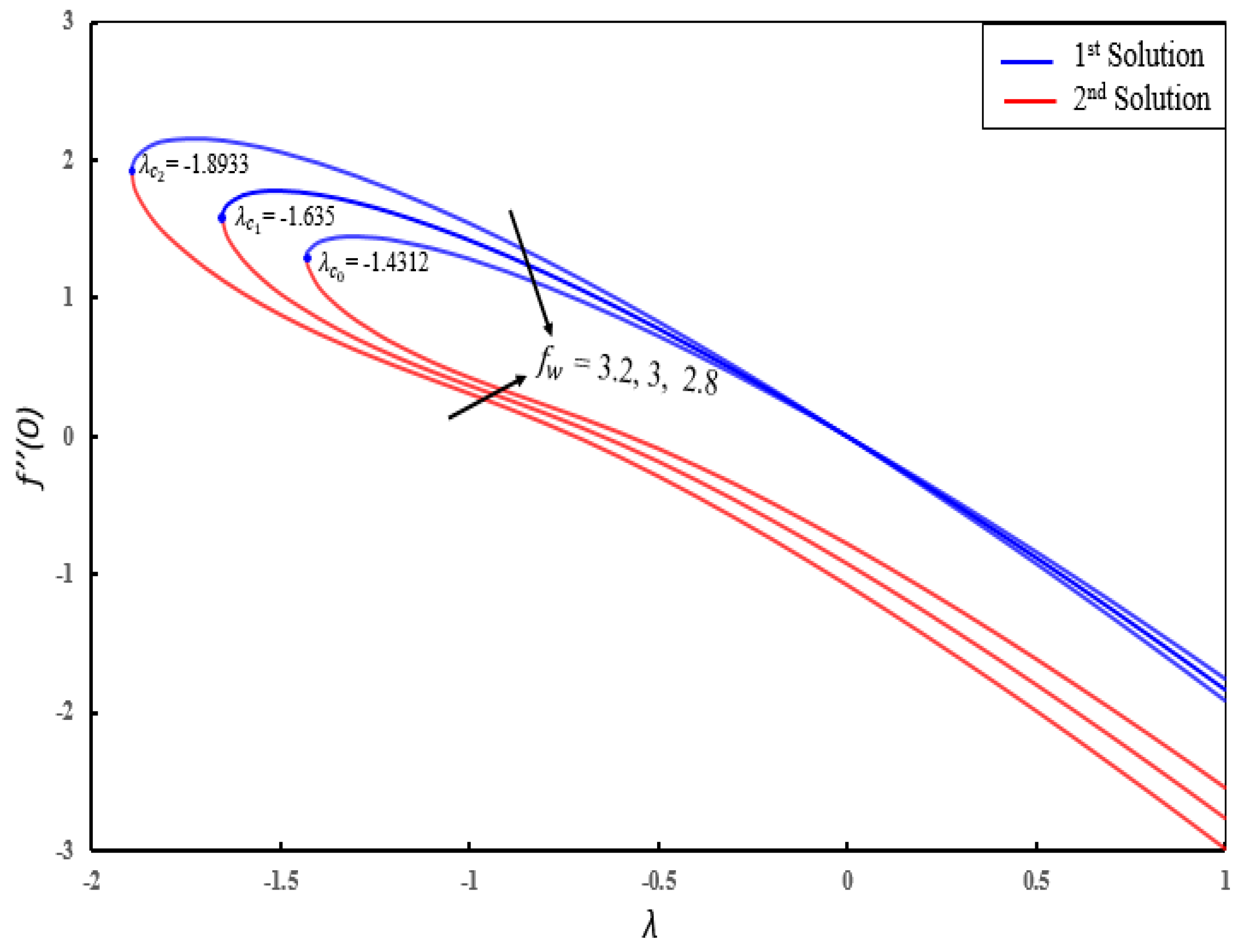
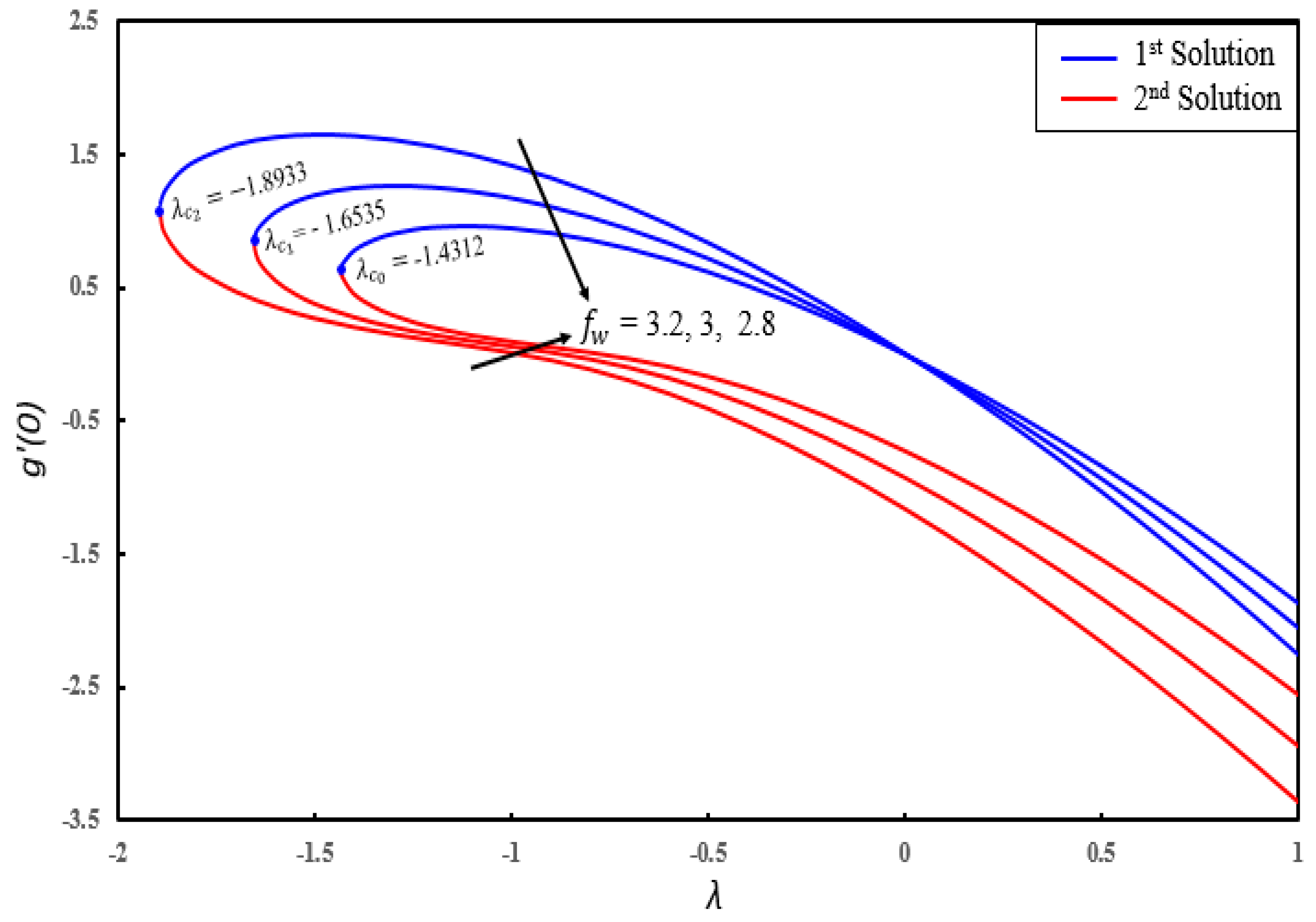
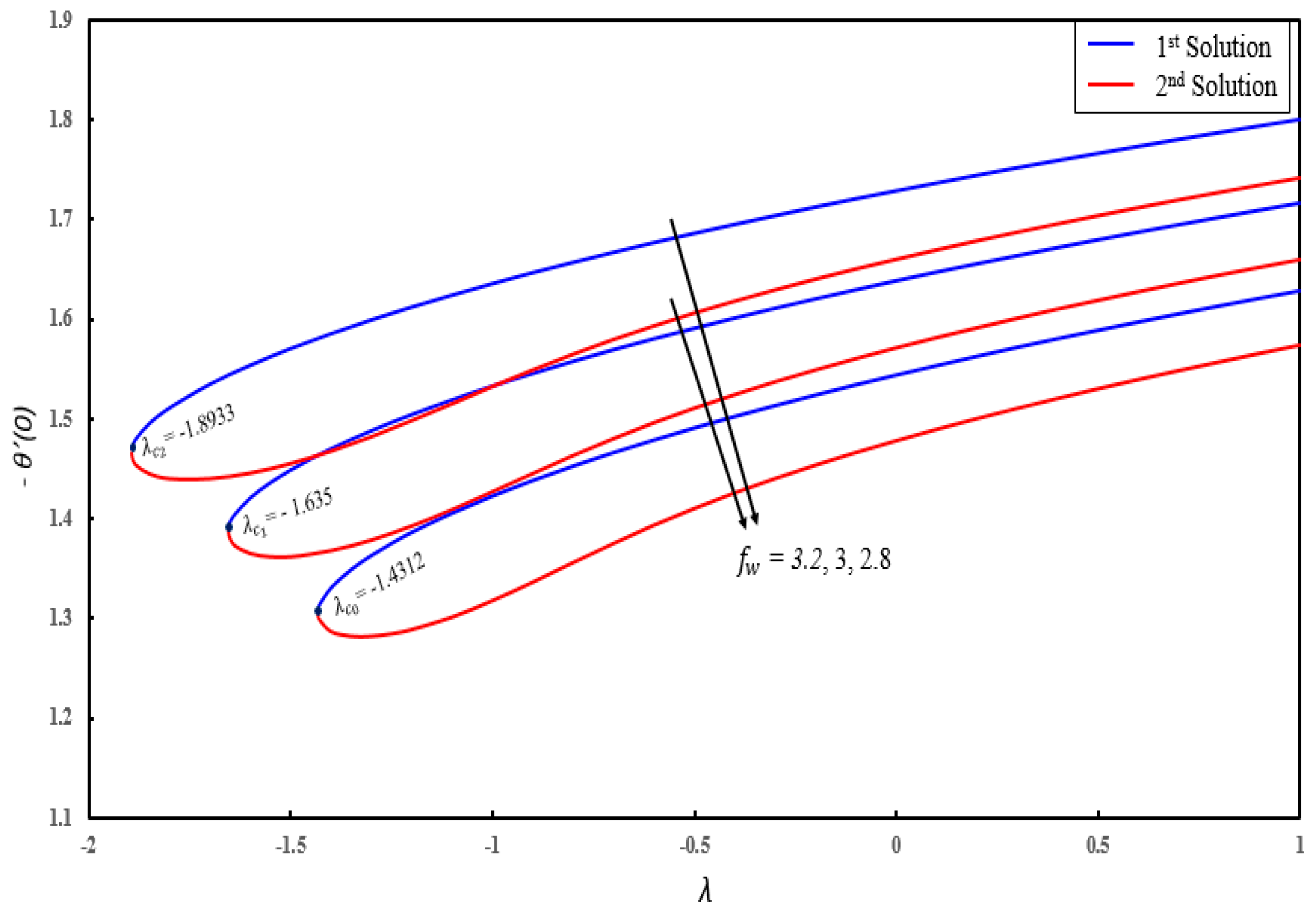
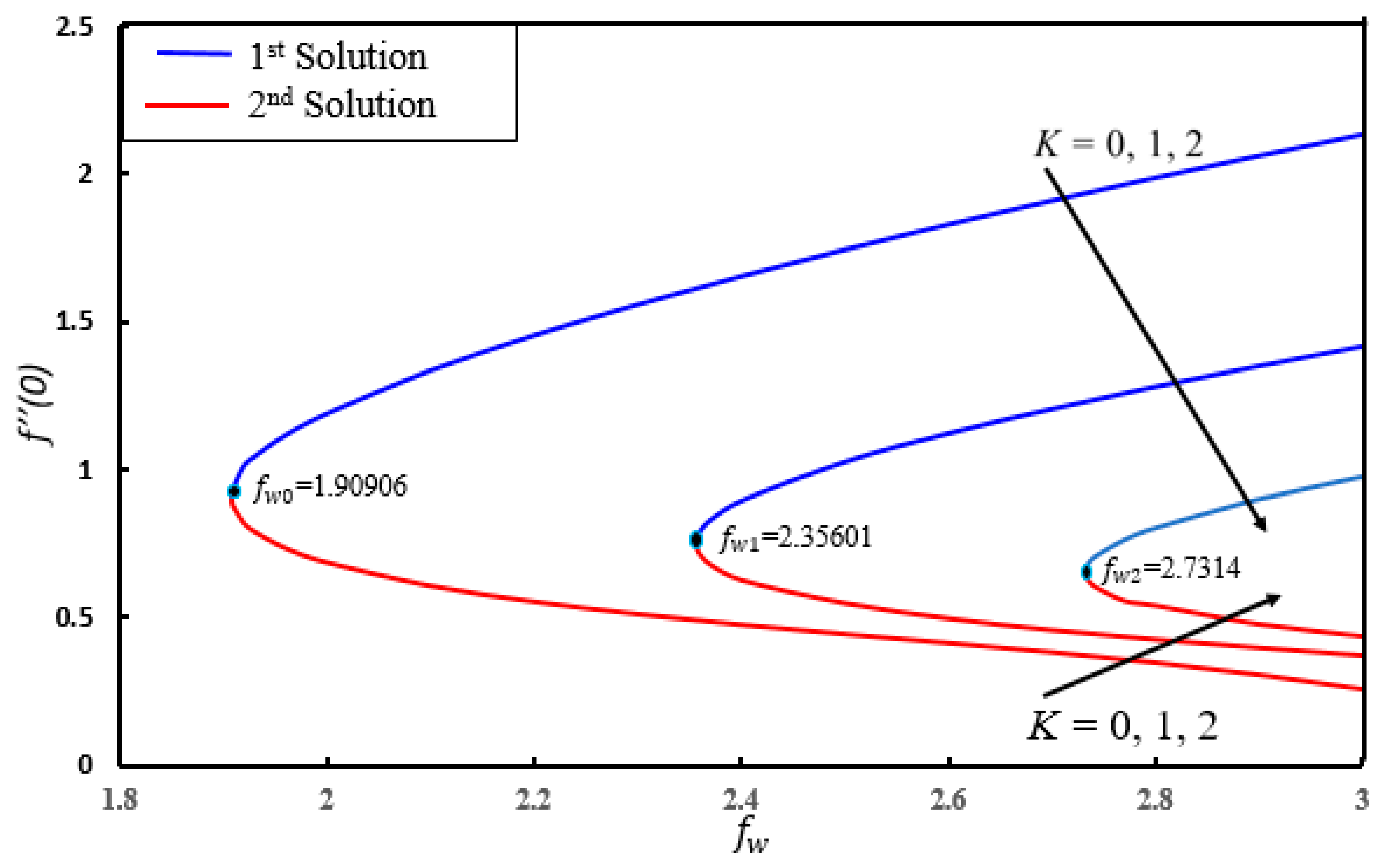
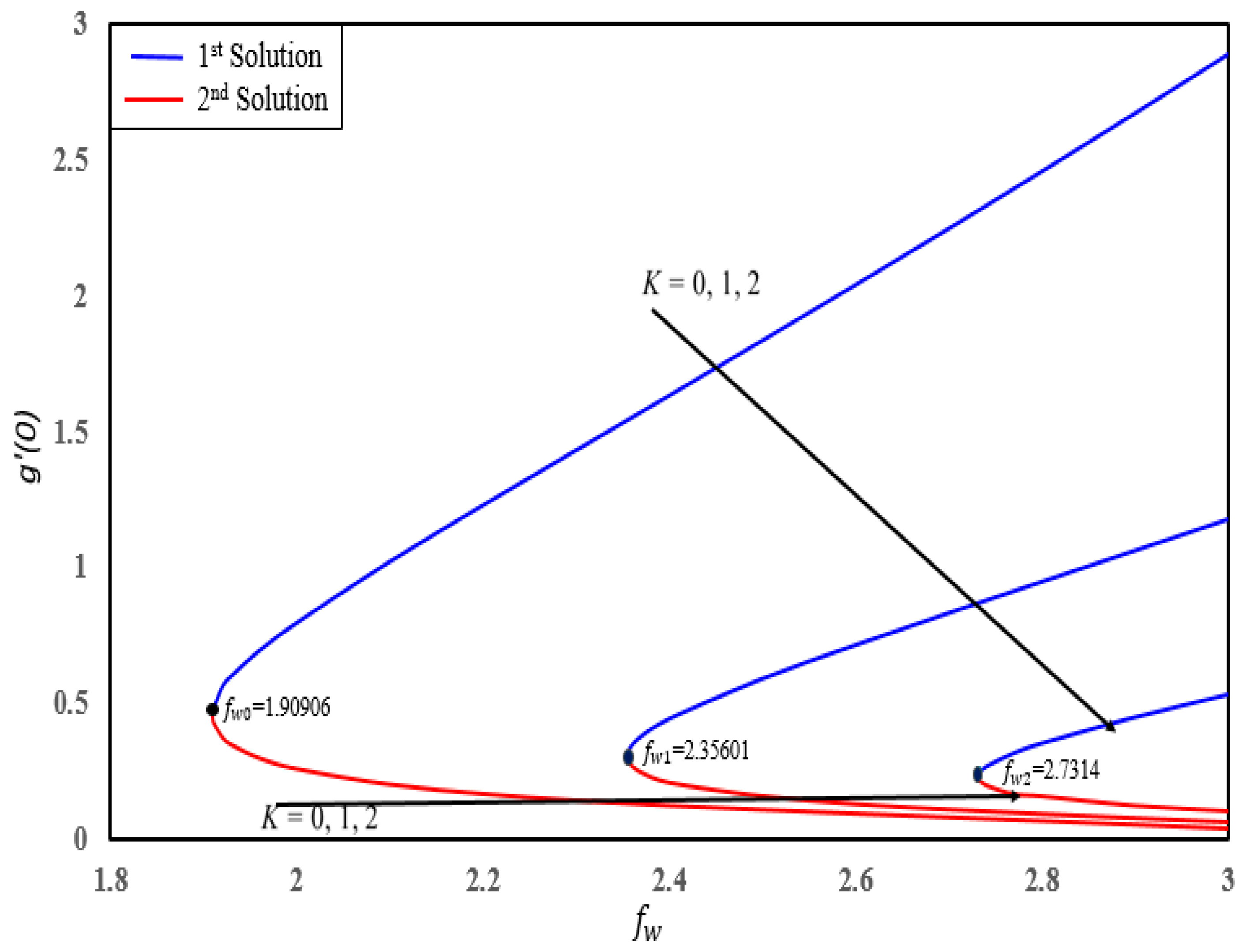
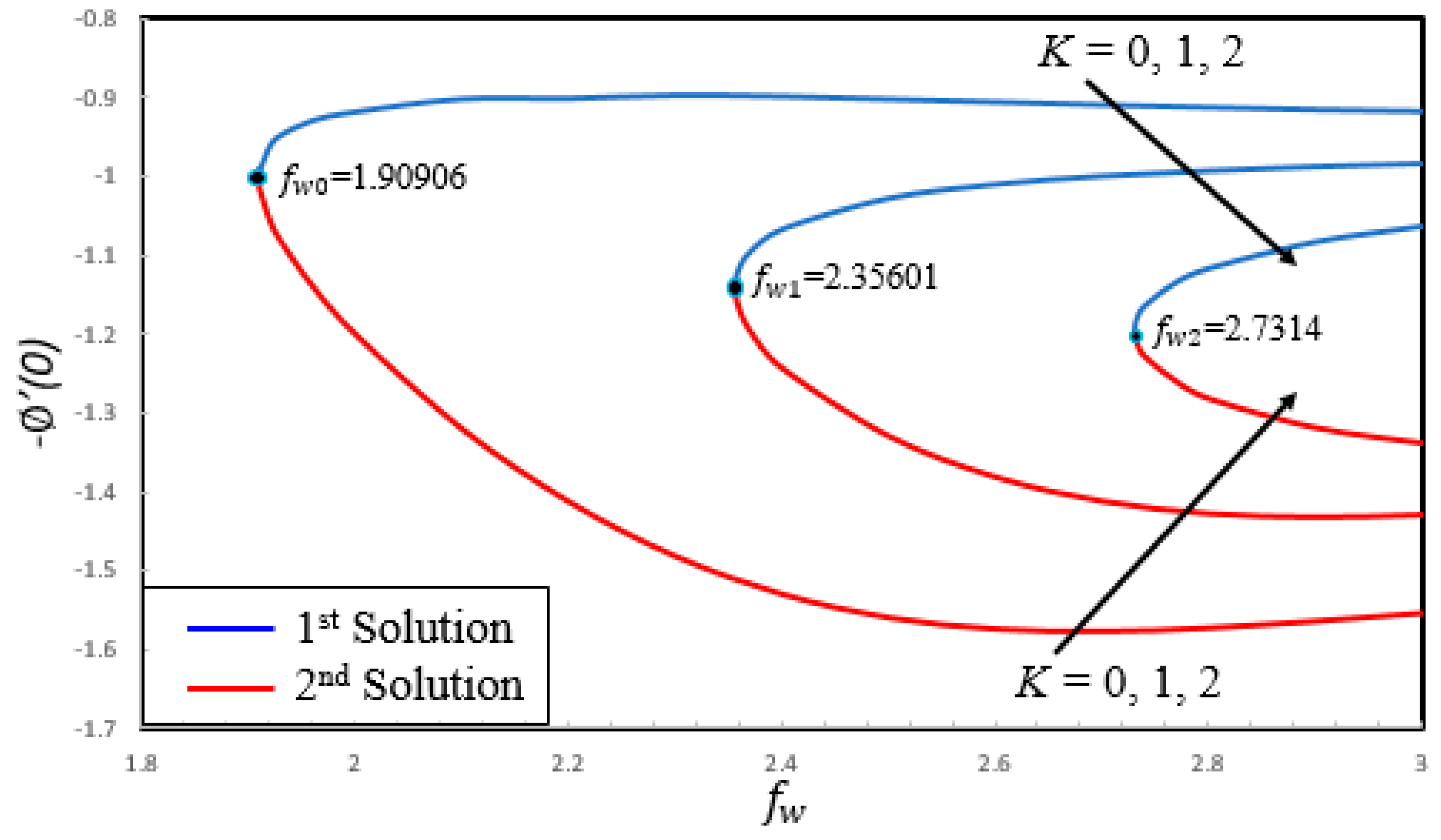
• Dual solutions exist for skin friction coefficient, couple stress coefficient, local Nusselt number and local Sherwood number for certain parameters.
• From stability analysis, it is examined that the first solution is stable and physically realizable, while the second solution is not stable so it is not physical realizable.
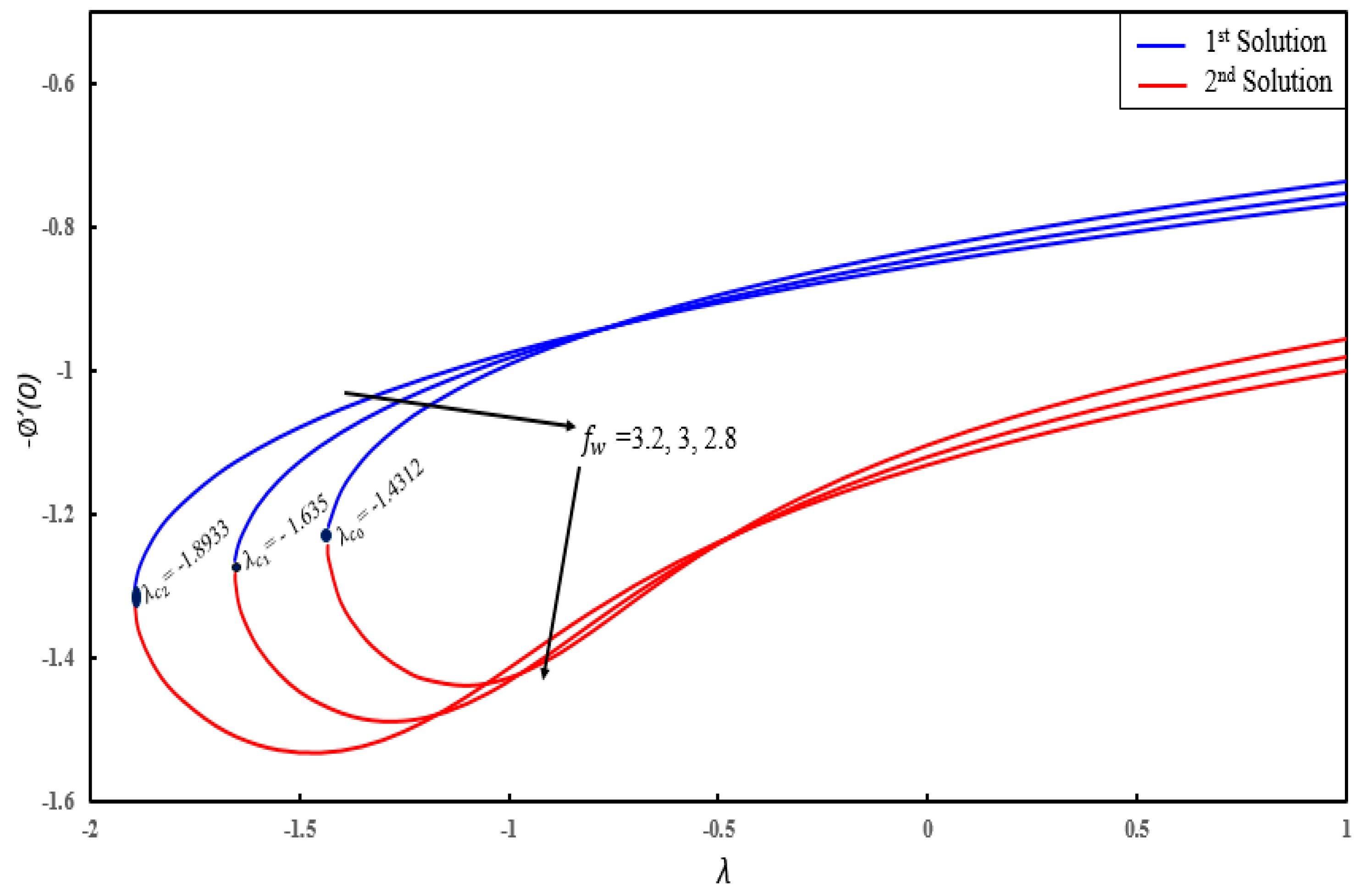
• There exist different ranges of dual similarity solutions. For $K=1$ ($K=2$), dual solutions occur when $f_w\ge 2.35601$ ($f_w\ge 2.7314$) and no solution when $f_w<2.35601(f_w<2.7314)$.
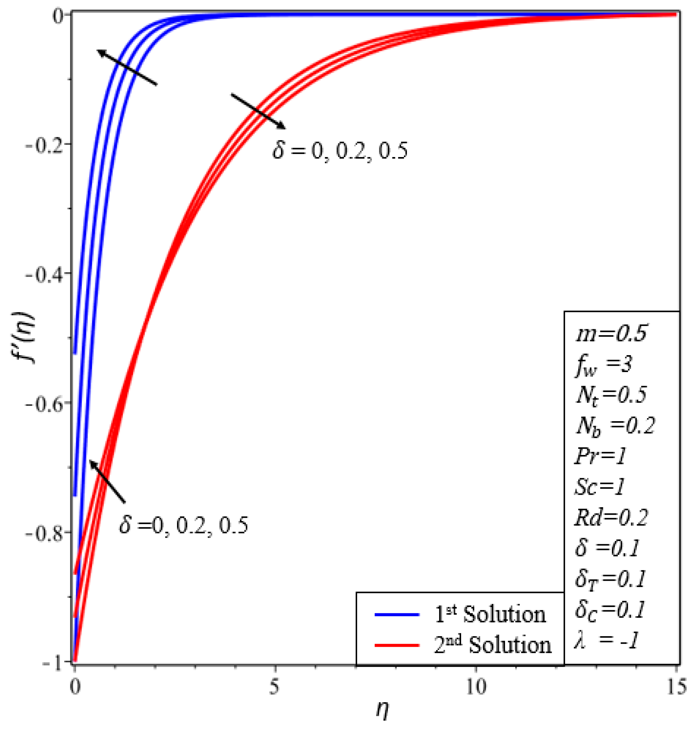
• The velocity profile declines in the first solution by increasing the values of the velocity slip parameter.
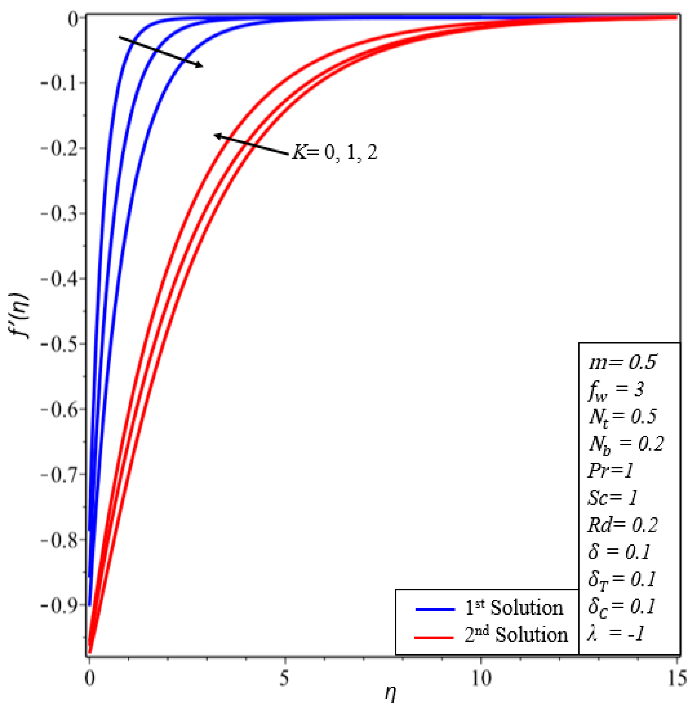
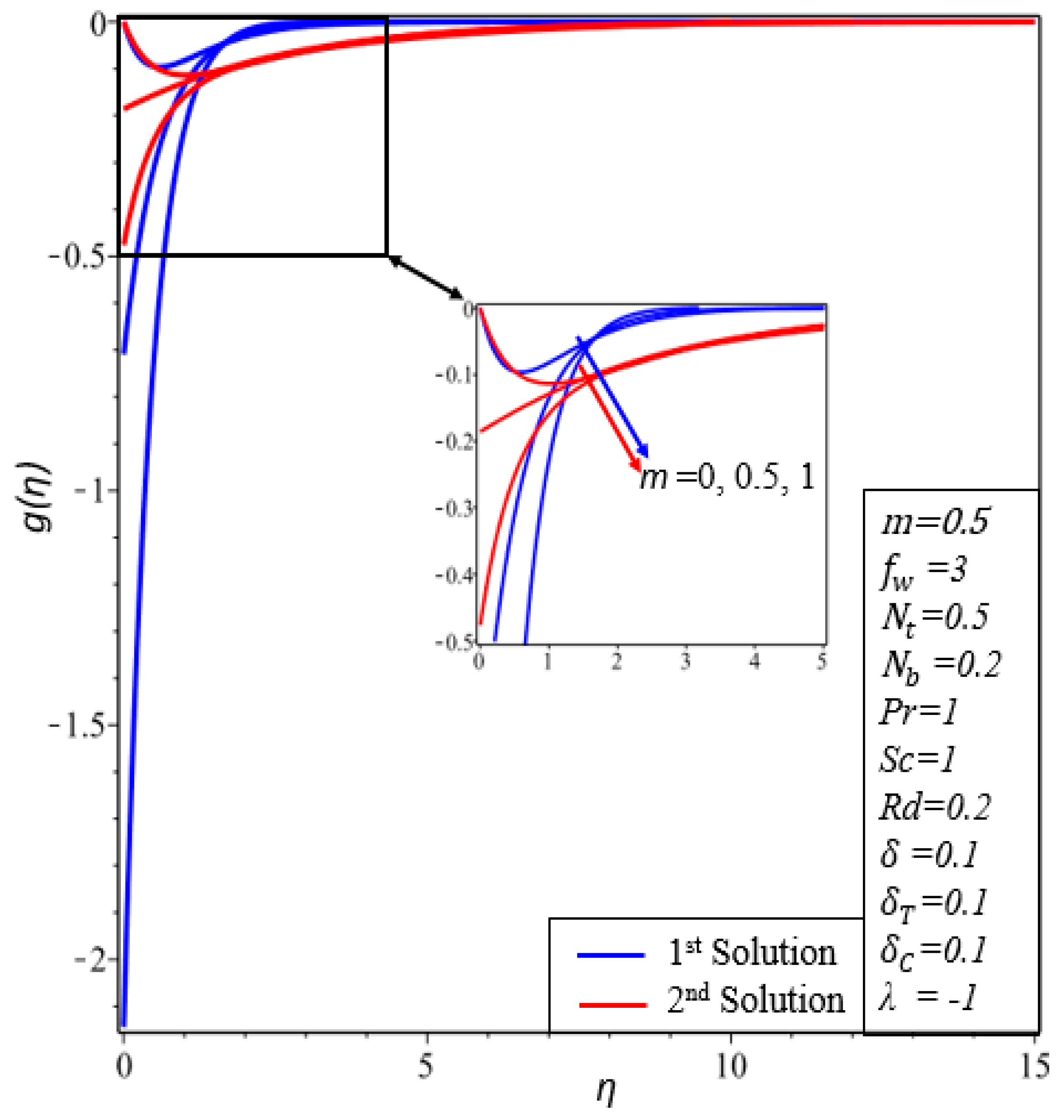
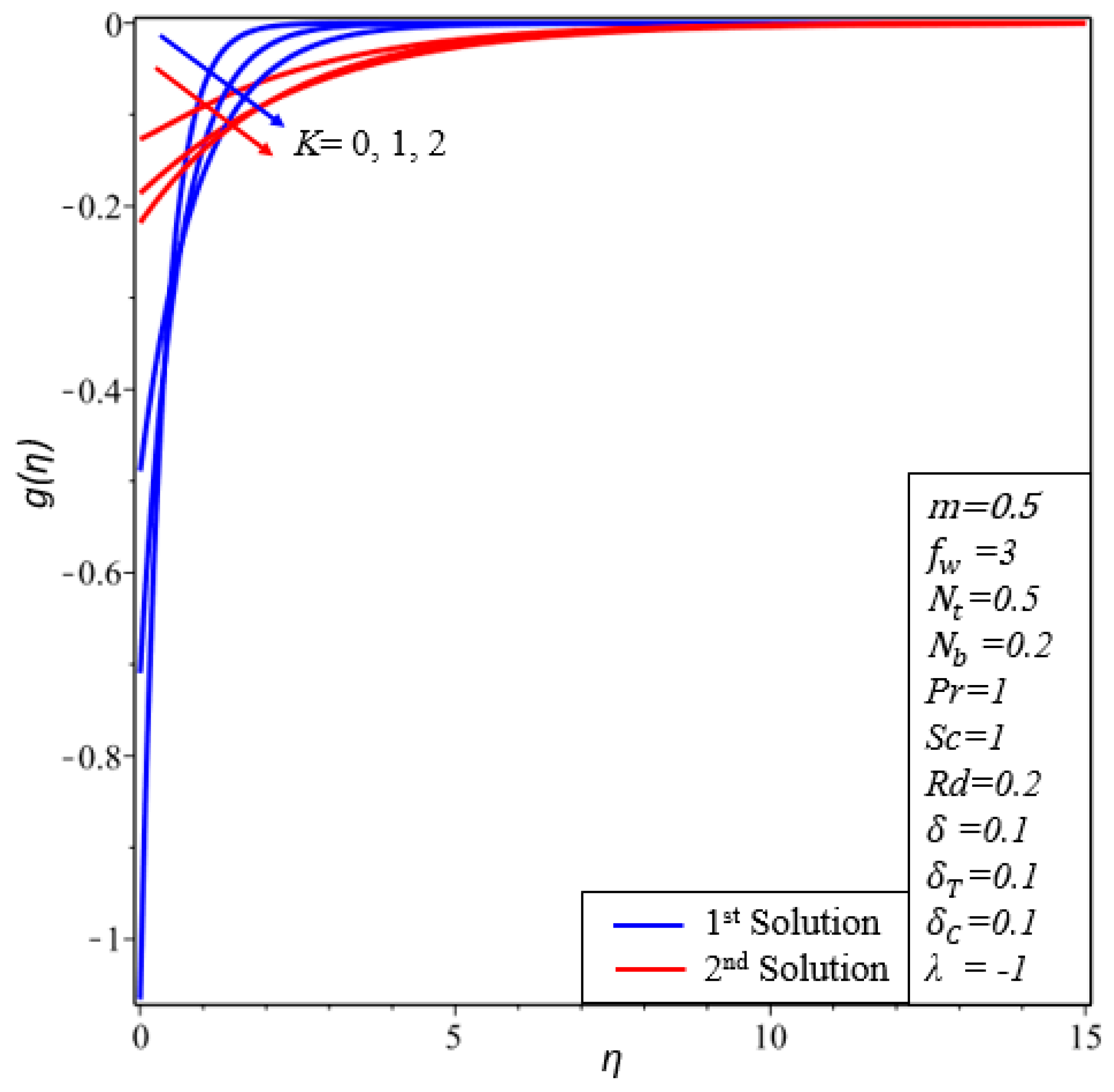
• The impact of $m$ and $K$ on microrotation profiles show that the microrotation boundary layer thicknesses and microrotation profiles decrease in both solutions.
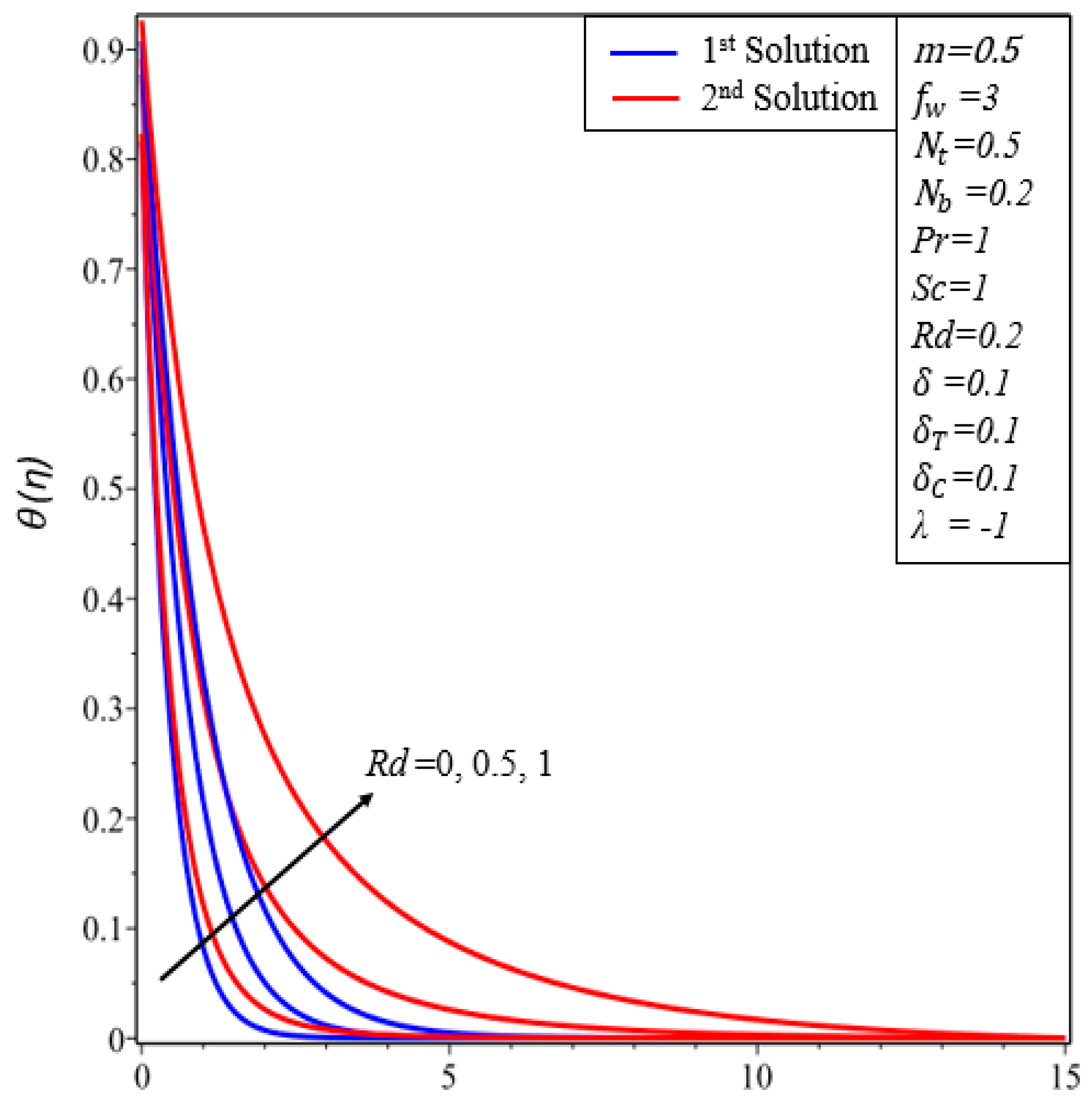
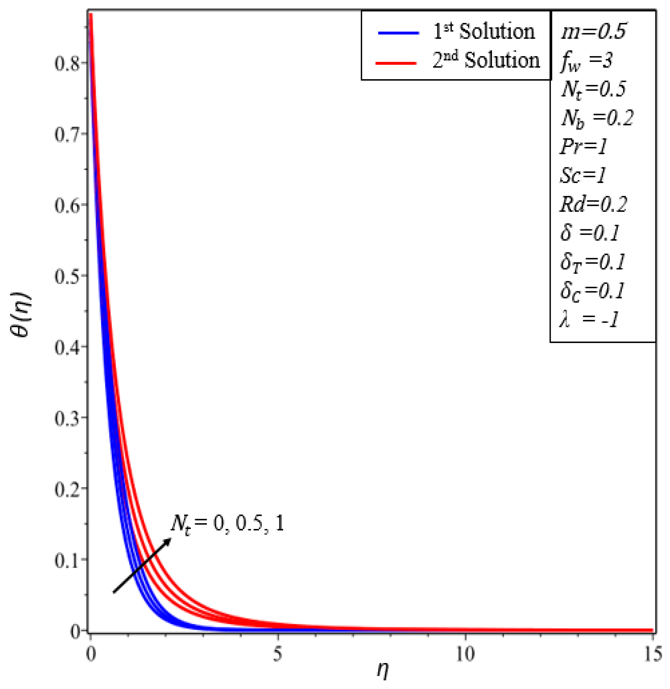
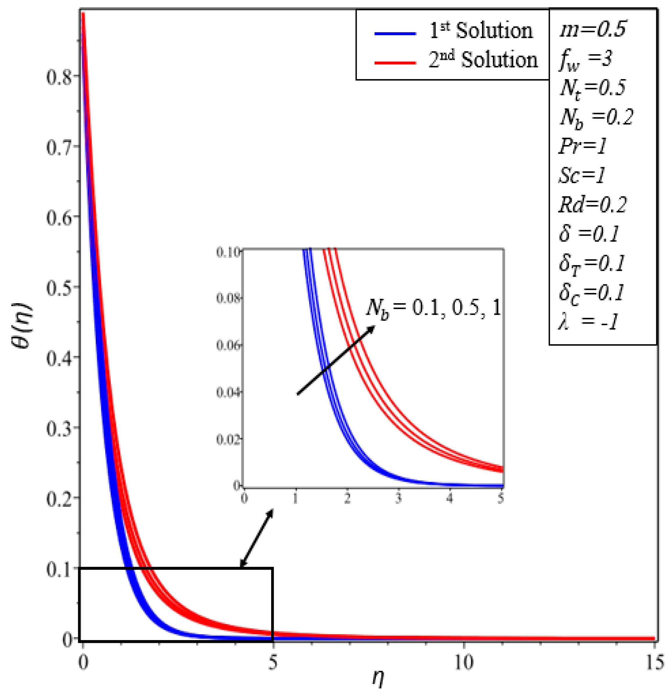
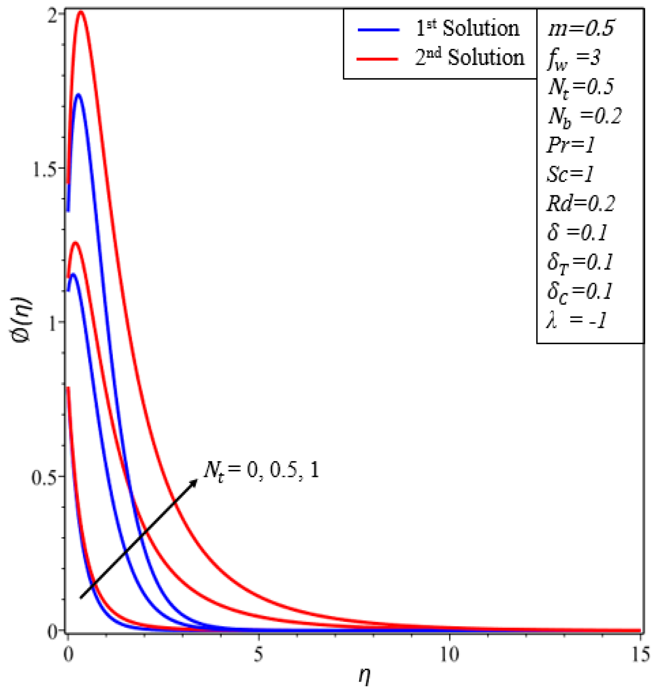
• Temperature profiles increase in both solutions when thermal radiation, thermophoresis and the Brownian motion parameters are enhanced.
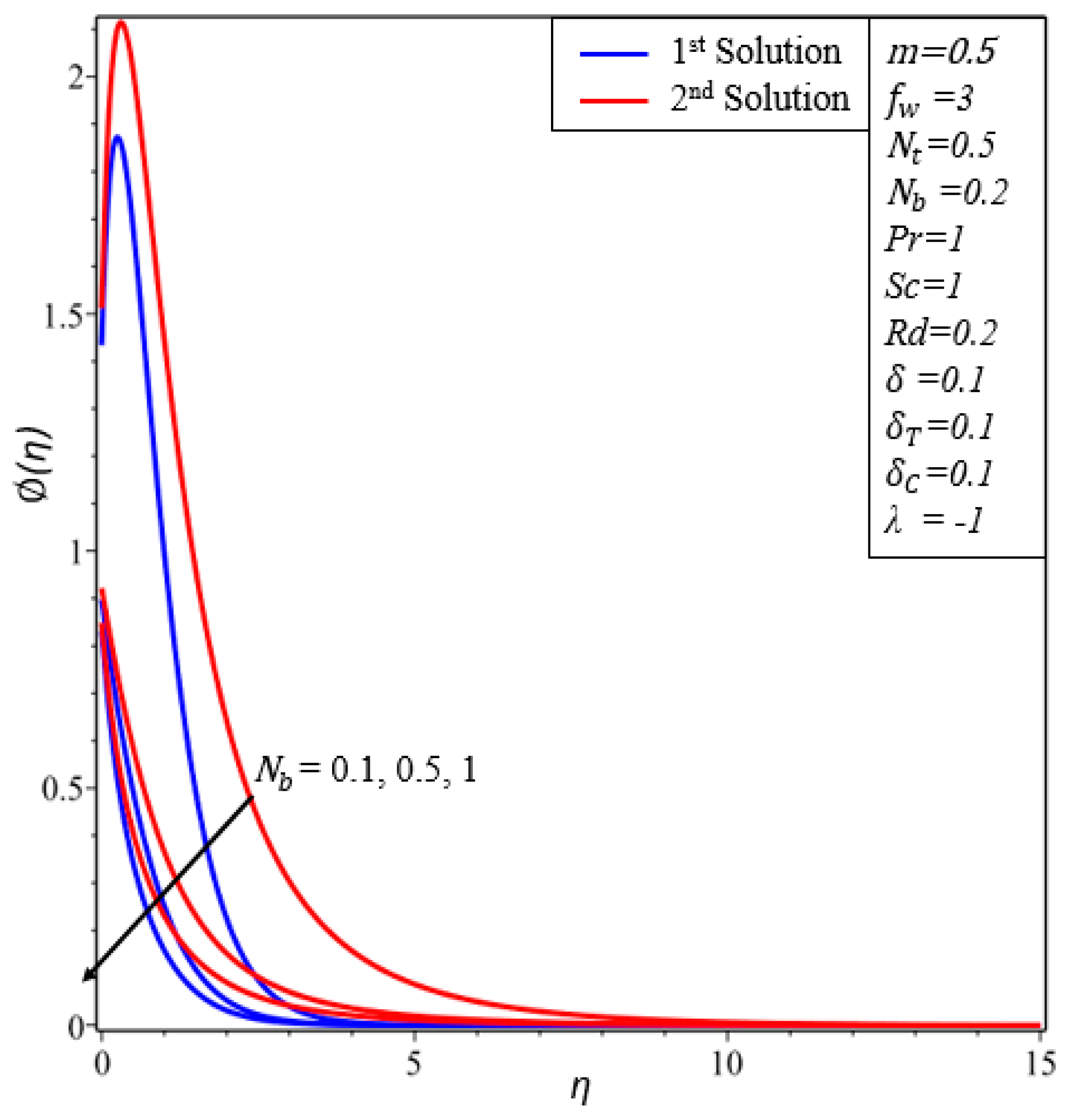
• The concentration of nanoparticles increases by increasing $N_t$ and decreases by increasing $N_b.$

References

- Eringen, A.C. Theory of thermomicrofluids. J. Math. Anal. Appl. 1972, 38, 480–496. [Google Scholar] [CrossRef]
- Chol, S.U.S.; Estman, J.A. Enhancing thermal conductivity of fluids with nanoparticles. ASME Publ. Fed. 1995, 231, 99–106. [Google Scholar]
- Tiwari, R.K.; Das, M.K. Heat transfer augmentation in a two-sided lid-driven differentially heated square cavity utilizing nanofluids. Int. J. Heat Mass Transf. 2007, 50, 2002–2018. [Google Scholar] [CrossRef]
- Buongiorno, J. Convective transport in nanofluids. J. Heat Transf. 2006, 128, 240–250. [Google Scholar] [CrossRef]
- Salleh, S.N.A.; Bachok, N.; Arifin, N.M.; Ali, F.M.; Pop, I. Magnetohydrodynamics Flow Past a Moving Vertical Thin Needle in a Nanofluid with Stability Analysis. Energies 2018, 11, 3297. [Google Scholar] [CrossRef]
- Hsiao, K.-L. Micropolar nanofluid flow with MHD and viscous dissipation effects towards a stretching sheet with multimedia feature. Int. J. Heat Mass Transf. 2017, 112, 983–990. [Google Scholar] [CrossRef]
- Lund, L.A.; Omar, Z.; Khan, I.; Raza, J.; Bakouri, M.; Tlili, I. Stability Analysis of Darcy-Forchheimer Flow of Casson Type Nanofluid Over an Exponential Sheet: Investigation of Critical Points. Symmetry 2019, 11, 412. [Google Scholar] [CrossRef]
- Lund, L.A.; Omar, Z.; Khan, I.; Khan, I. Analysis of dual solution for MHD flow of Williamson fluid with slippage. Heliyon 2019, 5, e01345. [Google Scholar] [CrossRef]
- Hashemi, H.; Namazian, Z.; Mehryan, S. Cu-water micropolar nanofluid natural convection within a porous enclosure with heat generation. J. Mol. Liq. 2017, 236, 48–60. [Google Scholar] [CrossRef]
- Hussain, S.T.; Nadeem, S.; Haq, R.U. Model-based analysis of micropolar nanofluid flow over a stretching surface. Eur. Phys. J. Plus 2014, 129, 161. [Google Scholar] [CrossRef]
- Dero, S.; Uddin, M.J.; Rohni, A.M. Stefan Blowing and Slip Effects on Unsteady Nanofluid Transport Past a Shrinking Sheet: Multiple Solutions. Heat Transf. Asian Res. 2019, 48, 2047–2066. [Google Scholar] [CrossRef]
- Dero, S.; Rohni, A.M.; Saaban, A. MHD Micropolar Nanofluid Flow over an Exponentially Stretching/Shrinking Surface: Triple Solutions. J. Adv. Res. Fluid Mech. Therm. Sci. 2019, 56, 165–174. [Google Scholar]
- Dero, S.; Rohni, A.M.; Saaban, A. The Dual Solutions and Stability Analysis of Nanofluid Flow using Tiwari-Das Modelover a Permeable Exponentially Shrinking Surface with Partial Slip Conditions. J. Eng. Appl. Sci. 2019, 14, 4569–4582. [Google Scholar]
- Alarifi, I.M.; Alkouh, A.B.; Ali, V.; Nguyen, H.M.; Asadi, A. On the rheological properties of MWCNT-TiO2/oil hybrid nanofluid: An experimental investigation on the effects of shear rate, temperature, and solid concentration of nanoparticles. Powder Technol. 2019, 355, 157–162. [Google Scholar] [CrossRef]
- Pourfattah, F.; Arani, A.A.A.; Babaie, M.R.; Nguyen, H.M.; Asadi, A. On the thermal characteristics of a manifold microchannel heat sink subjected to nanofluid using two-phase flow simulation. Int. J. Heat Mass Transf. 2019, 143, 118518. [Google Scholar] [CrossRef]
- Alsarraf, J.; Moradikazerouni, A.; Shahsavar, A.; Afrand, M.; Salehipour, H.; Tran, M.D. Hydrothermal analysis of turbulent boehmite alumina nanofluid flow with different nanoparticle shapes in a minichannel heat exchanger using two-phase mixture model. Phys. A Stat. Mech. Appl. 2019, 520, 275–288. [Google Scholar] [CrossRef]
- Jafarimoghaddam, A. Two-phase modeling of magnetic nanofluids jets over a Stretching/shrinking wall. Therm. Sci. Eng. Prog. 2018, 8, 375–384. [Google Scholar] [CrossRef]
- Jafarimoghaddam, A.; Pop, I. Numerical modeling of Glauert type exponentially decaying wall jet flows of nanofluids using Tiwari and Das’ nanofluid model. Int. J. Numer. Methods Heat Fluid Flow 2019, 29, 1010–1038. [Google Scholar] [CrossRef]
- Pal, D.; Mandal, G. Thermal radiation and MHD effects on boundary layer flow of micropolar nanofluid past a stretching sheet with non-uniform heat source/sink. Int. J. Mech. Sci. 2017, 126, 308–318. [Google Scholar] [CrossRef]
- Moradikazerouni, A.; Hajizadeh, A.; Safaei, M.R.; Afrand, M.; Yarmand, H.; Zulkifli, N.W.B.M. Assessment of thermal conductivity enhancement of nano-antifreeze containing single-walled carbon nanotubes: Optimal artificial neural network and curve-fitting. Phys. A Stat. Mech. Appl. 2019, 521, 138–145. [Google Scholar] [CrossRef]
- Asadi, A.; Aberoumand, S.; Moradikazerouni, A.; Pourfattah, F.; Żyła, G.; Estellé, P.; Mahian, O.; Wongwises, S.; Nguyen, H.M.; Arabkoohsar, A. Recent advances in preparation methods and thermophysical properties of oil-based nanofluids: A state-of-the-art review. Powder Technol. 2019, 352, 209–226. [Google Scholar] [CrossRef]
- Vo, D.D.; Alsarraf, J.; Moradikazerouni, A.; Afrand, M.; Salehipour, H.; Qi, C. Numerical investigation of γ-AlOOH nano-fluid convection performance in a wavy channel considering various shapes of nanoadditives. Powder Technol. 2019, 345, 649–657. [Google Scholar] [CrossRef]
- Awais, M.; Hayat, T.; Ali, A.; Irum, S. Velocity, thermal and concentration slip effects on a magneto-hydrodynamic nanofluid flow. Alex. Eng. J. 2016, 55, 2107–2114. [Google Scholar] [CrossRef]
- Das, K. Slip effects on MHD mixed convection stagnation point flow of a micropolar fluid towards a shrinking vertical sheet. Comput. Math. Appl. 2012, 63, 255–267. [Google Scholar] [CrossRef][Green Version]
- Ramya, D.; Raju, R.S.; Rao, J.A.; Chamkha, A. Effects of velocity and thermal wall slip on magnetohydrodynamics (MHD) boundary layer viscous flow and heat transfer of a nanofluid over a non-linearly-stretching sheet: A numerical study. Propuls. Power Res. 2018, 7, 182–195. [Google Scholar] [CrossRef]
- Ramzan, M.; Chung, J.D.; Ullah, N. Partial slip effect in the flow of MHD micropolar nanofluid flow due to a rotating disk – A numerical approach. Results Phys. 2017, 7, 3557–3566. [Google Scholar] [CrossRef]
- Sui, J.; Zhao, P.; Cheng, Z.; Doi, M. Influence of particulate thermophoresis on convection heat and mass transfer in a slip flow of a viscoelasticity-based micropolar fluid. Int. J. Heat Mass Transf. 2018, 119, 40–51. [Google Scholar] [CrossRef]
- Ramzan, M.; Farooq, M.; Hayat, T.; Chung, J.D. Radiative and Joule heating effects in the MHD flow of a micropolar fluid with partial slip and convective boundary condition. J. Mol. Liq. 2016, 221, 394–400. [Google Scholar] [CrossRef]
- Lund, L.A.; Omar, Z.; Khan, I. Mathematical analysis of magnetohydrodynamic (MHD) flow of micropolar nanofluid under buoyancy effects past a vertical shrinking surface: Dual solutions. Heliyon 2019, 5, 02432. [Google Scholar] [CrossRef]
- Hayat, T.; Khan, M.I.; Waqas, M.; Alsaedi, A.; Khan, M.I. Radiative flow of micropolar nanofluid accounting thermophoresis and Brownian moment. Int. J. Hydrogen Energy 2017, 42, 16821–16833. [Google Scholar] [CrossRef]
- Ramzan, M.; Ullah, N.; Chung, J.D.; Lu, D.; Farooq, U. Buoyancy effects on the radiative magneto Micropolar nanofluid flow with double stratification, activation energy and binary chemical reaction. Sci. Rep. 2017, 7, 12901. [Google Scholar] [CrossRef] [PubMed]
- Weidman, P.; Kubitschek, D.; Davis, A. The effect of transpiration on self-similar boundary layer flow over moving surfaces. Int. J. Eng. Sci. 2006, 44, 730–737. [Google Scholar] [CrossRef]
- Roşca, N.C.; Pop, I. Mixed convection stagnation point flow past a vertical flat plate with a second order slip: Heat flux case. Int. J. Heat Mass Transf. 2013, 65, 102–109. [Google Scholar] [CrossRef]
- Roşca, A.V.; Pop, I. Mixed Convection Stagnation-Point Flow Past a Vertical Flat Plate with a Second Order Slip. J. Heat Transf. 2014, 136, 012501. [Google Scholar] [CrossRef]
- Harris, S.D.; Ingham, D.B.; Pop, I. Mixed convection boundary-layer flow near the stagnation point on a vertical surface in a porous medium: Brinkman model with slip. Transp. Porous Media 2009, 77, 267–285. [Google Scholar] [CrossRef]
- Lund, L.A.; Ching, D.L.C.; Omar, Z.; Khan, I.; Nisar, K.S.; Khan, I.; Khan, I. Triple Local Similarity Solutions of Darcy-Forchheimer Magnetohydrodynamic (MHD) Flow of Micropolar Nanofluid Over an Exponential Shrinking Surface: Stability Analysis. Coatings 2019, 9, 527. [Google Scholar] [CrossRef]
- Lund, L.A.; Omar, Z.; Khan, I. Quadruple solutions of mixed convection flow of magnetohydrodynamic nanofluid over exponentially vertical shrinking and stretching surfaces: Stability analysis. Comput. Methods Progr. Biomed. 2019, 182, 105044. [Google Scholar] [CrossRef]
- Lund, L.A.; Omar, Z.; Khan, I.; Dero, S. Multiple solutions of Cu-C6H9NaO7 and Ag-C6H9NaO7 nanofluids flow over nonlinear shrinking surface. J. Cent. South Univ. 2019, 26, 1283–1293. [Google Scholar] [CrossRef]