Experimental Demonstration of Deterministic Chaos in a Waste Oil Biodiesel Semi-Industrial Furnace Combustion System

Abstract

In this paper, the nonlinear dynamic characteristics of the oxygen-enriched combustion of waste oil biodiesel in semi-industrial furnaces were tested by the power spectrum, phase space reconstruction, the largest Lyapunov exponents, and the 0-1 test method. To express the influences of the system parameters, experiments were carried out under different oxygen content conditions (21%, 25%, 28%, 31%, and 33%). Higher oxygen enrichment degrees contribute to finer combustion sufficiency, which produces flames with high luminance. Flame luminance and temperature can be represented by different gray scale values of flame images. The chaotic characteristics of gray scale time series under different oxygen enrichment degrees were studied. With increased oxygen content, the chaotic characteristics of flame gradually developed from weak chaos to strong chaos. Furthermore, the flame maintained a stable combustion process in a high-temperature region. The stronger the chaotic characteristics of the flame, the better the combustion effect. It can be seen that the change of initial combustion conditions has a great influence on the whole combustion process. The results of several chaotic test methods were consistent. Using chaotic characteristics to analyze the waste oil biodiesel combustion process can digitize the combustion process, find the best combustion state, optimize, and precisely control it.

1. Introduction

In recent years, oil shortages and environmental pollution have become two major challenges of mankind. There is an urgent need to find alternative fuels for industrial furnaces for the development of modern society. Vigorously developing biodiesel has important strategic significance for sustainable economic development, promoting energy substitution, reducing environmental pressure, and controlling urban air pollution [1,2]. As the global demands for environmental protection, energy conservation, and emission reduction become higher, it is urgent to develop a new generation of biodiesel combustion monitoring technology [3]. Due to the complexity of the biodiesel combustion situation, how to preserve normal combustion and extract the information in the combustion process effectively is a difficult problem. At this time, advanced combustion diagnosis technology is critical. On the one hand, different characteristics of the combustion process will be found through combustion diagnostic techniques. This will improve the cognition of physical combustion phenomena used to test numerical and theoretical models. On the other hand, the relationship of combustion results such as flame stability, combustion efficiency, and pollutant emissions with initial conditions can be found. Through appropriate processing and calibration methods, these features can be used to implement monitoring algorithms to improve the security and reliability of combustion facilities [4,5]. Zhang (2012) used a high-speed camera to record flame images and analyzed variations of flame volume, shape, structure, and length under different atomization pressures and air excess coefficients. The results showed that the flame volume gradually decreased with increased excess air coefficient under the same atomization pressure. [6]. Wang (2013) used a high-speed camera to record flame images to study the change rule of air preheating temperature on the shape, length, and area of biodiesel combustion flame. The results showed that with increased preheating temperature, the flame shape gradually became compact from dispersion. The flame length and area both decreased first and then increased with the increased preheating temperature [7]. Jiang et al. (2015) studied the change rule of the temperature field in the flame area when biodiesel was burned in a kiln via a swirl burner and analyzed the influence of different excess air coefficients and combustion air temperatures on the temperature field in the flame area [8]. Jiang et al. (2013) studied the emission characteristics of CO and NO from biodiesel combustion in kilns. The results showed that with increased air excess coefficient, CO emission first decreased and then increased, while NO emission first increased and then decreased [9]. Ibrahim (2016) studied and compared the performance, combustion characteristics, NOx emissions, and stability of diesel engines filled with five different biodiesel fuels [10]. Calder et al. (2018) conducted research on reducing NOx emissions of palm oil methyl ester mixed with diesel oil and improving the ignition performance of test fuel [11]. Qubeissi et al. (2018) mainly studied the heating and evaporation of automobile fuel droplets. Several kinds of mixed biodiesel fuels were added and the combustion of internal combustion engines was experimentally studied [12]. Kilic et al. (2018) conducted an experimental study on the combustion of butanol/diesel/biodiesel blends and explored their effects on the boiler performance and emission performance of reverse flame tube boilers [13]. Jeon et al. (2018) used a visualization system to analyze spatial combustion flame and investigated B20 combustion and soot emission processes under different injection pressure conditions [14].

By determining whether the combustion process of biodiesel is random, regular, or chaotic, useful strategies and short-term predictions can be provided for combustion in industrial production. Nonlinear deterministic and chaotic characteristics in the combustion process have been shown in many studies [15,16,17,18,19,20]. Currently, chaotic features can be identified by different methods and standards, such as Lorenz map [21], Poincare map [22], Grassberger-Procaccia algorithm [23], power spectrum and strange attractor [24], and Lyapunov stabilization [25,26].

Cheng et al. (2016) used evolutionary support vector machine to establish a high-precision prediction model, obtaining an optimal mixed performance prediction model through the K-means chaos genetic algorithm [27]. The chaotic characteristics of combustion were analyzed by a nonlinear method and the related trends were predicted by Maheshwari et al. (2011) [28] and Kabiraj et al. (2012) [29]. Davies (2000) used an improved simple proportional feedback algorithm to control the chaotic evolution of carbon monoxide combustion experimentally in a well-stirred flow reactor [30].

A new method to replace the classical complex chaotic identification, named the 0-1 test, has been used to diagnose chaos in dynamical systems that do not require phase space reconstruction. Gottwald and Melbourne (2009a, 2009b) used this method to identify chaotic phenomena from regular behavior in deterministic systems [31,32,33]. The 0-1 detection method can judge whether the time series is chaotic without phase space reconstruction, and has been verified in the natural gas combustion process and many other fields [34,35,36].

The aim of this paper is to study the nonlinear fluctuation characteristics of the gray scale of waste oil biodiesel combustion flame images with continuously changing oxygen content, paying attention to the relationship between image flame characteristics and combustion performance parameters [37,38,39,40].

The paper is composed of the following parts: Section 2 introduces the experimental equipment, operating conditions, and image processing methods for extracting relevant flame parameters. In Section 3, different diagnostic tools for chaotic combustion are proposed. Section 4 presents the results and analysis. Section 5 summarizes conclusions and perspectives.

2. Experimental Apparatus, Operating Conditions

2.1. Experimental Apparatus

The burner design is mainly considered from two aspects: the first is the atomization effect of biodiesel, and the second is to provide sufficient combustion-supporting gas for the combustion of biodiesel. The internal structure of the burner consists of three layers of inner cavities. The innermost layer is a fuel channel through which high-pressure fuel is atomized once under the action of an atomizing nozzle. The middle layer is a primary combustion-supporting gas channel. The outlet side of the channel is provided with air swirl vanes. The air coming out of the swirl vanes is mixed with atomized fuel oil and plays a secondary role crushing the fuel oil, so the primary air function not only provides a certain amount of combustion-supporting gas for the combustion of biodiesel, but also can obviously improve the atomization effect. As the primary air outlet aperture is small, the primary air volume is insufficient to provide the quantity of air required for combustion. Therefore, the outermost layer of the burner is provided with a secondary air channel, which has a large space and can provide sufficient combustion-supporting gas for the combustion of biodiesel. An air baffle is also arranged at the outlet of the secondary air channel, and a circle of gas outlets is arranged around the baffle, so that a higher gas flow rate at the outlet can be ensured, and high-speed gas can accelerate the mixing of oil and gas, so that the combustion effect is better. Figure 1 shows the spray nozzle used in this waste oil biodiesel combustion experiment. Figure 2 shows the main flame monitoring system located in the combustion chamber.

2.2. Operating Conditions

In this paper, transesterification was used to prepare the waste oil biodiesel, and refined waste oil biodiesel was selected as the combustion agent. To provide a reliable theoretical basis for the design and subsequent tests of the combustion system, the physical parameters of waste oil biodiesel refer to the previous experimental data of our research group, as shown in

Table 1. Physical and chemical properties of fuel.

Name	Kinematic Viscosity	Surface Tension	Flash Point	Thermal Value	Condensation Point	Cetane Number
Waste oil biodiesel	4.61 m2/s	28.3 mN/m	152 °C	38.98 MJ/kg	6 °C	51

.

According to the stoichiometric number of complete combustion of waste oil biodiesel, the oxygen intake was selectively adjusted to make the oxygen enrichment degree 21%, 25%, 28%, 31%, and 33%.

2.3. Image Processing and Signal Analysis

As is known, MATLAB assigns an (i-j) pixel matrix to each image, where (i) is the row index and (j) is the column index. These values depend on image luminance between 0 and 255. In this range, the lowest correspond to dark pixels, and the highest correspond to light pixels. The luminance of the flame is represented by the gray value of the image in the image processing. The higher the gray value, the brighter the flame. In this paper, the luminance of the flame is expressed by the average gray scale method. The calculation method is to accumulate the gray value of each pixel point in the effective flame area in the image and compare the accumulated value with the pixel value in that area.

For an oil flame, with increased combustion temperature, the radiant energy emitted increases, which shows increased luminance (gray scale) on images obtained by the high-speed camera of PCO. The camera uses high-sensitivity, high-resolution, and high-speed CMOS sensors, which allows us to take high-definition images at a resolution of 1920 pixels × 1080 pixels with a maximum speed of 2128 frames per second. In this experiment, the image resolution was 1920 pixels × 1080 pixels and the shooting speed was 200 square seconds. Therefore, it can be considered that the gray scale value of the image is proportional to the temperature of the combustion flame. The principle of the calculation method consists of adding up the gray values of pixels in the valid flame area of the image and dividing the number of pixels in that area by the cumulative value to determine the average gray scale in the flame zone. According to actual flame images, areas with a gray scale higher than 70 are considered as combustion areas, and areas with a gray scale higher than 170 are considered as high-temperature areas. The high-temperature area is the complete burning area of the flame, which is the place with the greatest flame luminance. The backbone of the burning flame is the high-temperature area, where the gray scale changes little and the flicker frequency is low. The larger the area where the combustion flame has a stable high-temperature area, the stronger the flame’s ability to resist interference and the more stable the combustion. Generally speaking, under certain other conditions, the higher the combustion temperature, the more sufficient the combustion; that is to say, the higher the gray scale of the flame image, the more sufficient the combustion. As long as the burning flame has a certain stable high-temperature area, the flame will have strong resistance to interference and the combustion will be stable.

3. Diagnostic Tools

In this section, we talk about proven nonlinear indicators used to distinguish the chaotic combustion phenomenon.

3.1. Power Spectrum Analysis of Time Series

Signal spectrum analysis is an important part of digital signal processing. Some standard spectral techniques can be used to obtain the information of flame temporal dynamics. Characteristics such as maximum amplitude frequency, flicker frequency, and energy distribution according to spectral band can be acquired. The time domain representation of the signal is determined, and its spectrum can be obtained by MATLAB using fast Fourier transform (FFT). The frequency-domain representation of a signal reveals important characteristics that are difficult to analyze in the time domain.

Spectral density characterizes the frequency content of a signal or a stochastic process. Intuitively, the spectrum decomposes the signal or the stochastic process into different frequencies and identifies periodicities. There are a few algorithms for estimating the power spectral density (PSD) of a signal, including the Welch’s method, the periodogram, Yule-Walker autoregressive method, Burg method, etc. None of the PSD methods are perfect because they do not work as well for low signal to noise ratios and suffer from higher variance. Considering its simplicity, this paper used the periodogram, which is simple to implement in MATLAB. When there is a large number of signal time samples and the signal to noise ratio is high enough, this method can work well.

The power spectral density gives the energy distribution of time series in frequency. It is calculated as a discrete Fourier transform (DFT). Given a signal x(t_n) (n = 1, ..., N), obtained with sampling frequency f_s, DFT is defined as:

$$X\left(f_k\right)={{\displaystyle \sum }}_{i=1}^{N}x\left(t_n\right)e^{{-i2\pi f}_k{t}_n}\hspace{1em}k=0,1,2,\dots ,N-1,$$

(1)

where t_n indicates the time instantly, and f_k = k ∙ f_s/N is the corresponding frequency.

3.2. Reconstruction Phase Space

The purpose of phase space reconstruction is to restore the true trajectory of chaotic attractors in high-dimensional phase space, which is the basis of nonlinear dynamics analysis. Its basic principle is to find a nonlinear model in high-dimensional space, and use this model to re-display the dynamic characteristics of the system and realize prediction within a certain period of time. Embedding the gray scale time series of the flame image in the combustion process into m-dimensional space, a series of m-dimensional vectors of the phase space can be obtained to form the mathematical formula of the phase space of the system. The data points in the phase space can effectively restore the state of the system and predict its development trend with time through the movement rules of its data points. The motion law of each data point in the phase space finally forms the trajectory of the attractor of the high-dimensional system. Therefore, the development characteristics of the combustion flame and the motion relationship between front and back can be expressed by reconstructing the attractors in the phase space.

Given the time series x(j) (j = 1, 2, ..., N_m), one-dimensional time series is extended to m-dimensional phase space time series. According to Takens’s time-delay embedding theorem, by selecting the appropriate embedding dimension and time delay, the dynamic form of the original system can be restored in the sense of topological equivalence, so there is a smooth mapping F: R^m→ R^m, and the expression of phase space trajectory is given as follows:

X(j) = {x(j), x(j + τ), ⋯, x(j + (m − 1)τ)} j = 1, 2, 3, ⋯, N_m,

(2)

where X(j) is the m-dimensional vector, x(j) is the time series data point, m means the embedding dimension, and τ indicates the delay time; N_m = N − (m − 1) τ.

3.3. Largest Lyapunov Exponent

The Lyapunov exponent refers to the average rate of change of two trajectories that are close to each other in phase space. With the passage of time, the two trajectories separate or aggregate exponentially. When the variables evolve with time, the Lyapunov exponent spectrum of the system can effectively represent its sensitivity to initial values. An index less than zero indicates that the phase volume of the system shrinks in this direction and movement in this direction is stable. A positive exponential value indicates that the phase volume of the system expands and folds continuously in this direction, making the original adjacent trajectories in the attractor become increasingly irrelevant, thus making the initial state unpredictable with regard to the long-term behavior of the system; that is, so-called initial value sensitivity.

In this paper, based on Takens’s delayed coordinate reconstruction technique, m-dimensional phase space was reconstructed with delayed coordinates for turbulent flame image gray scale time series, the most suitable embedding dimension was calculated, and, finally, the Lyapunov exponent was calculated.

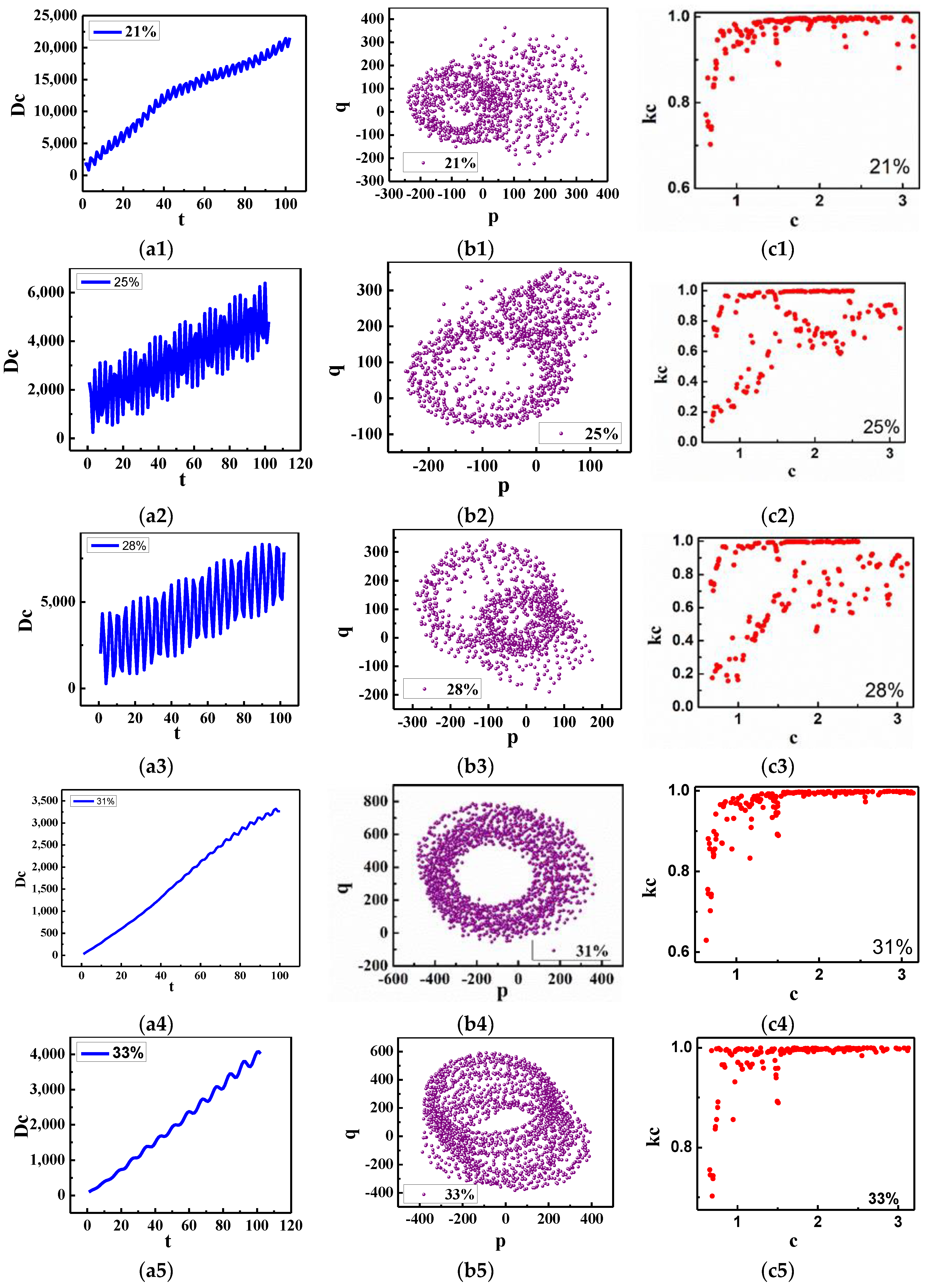
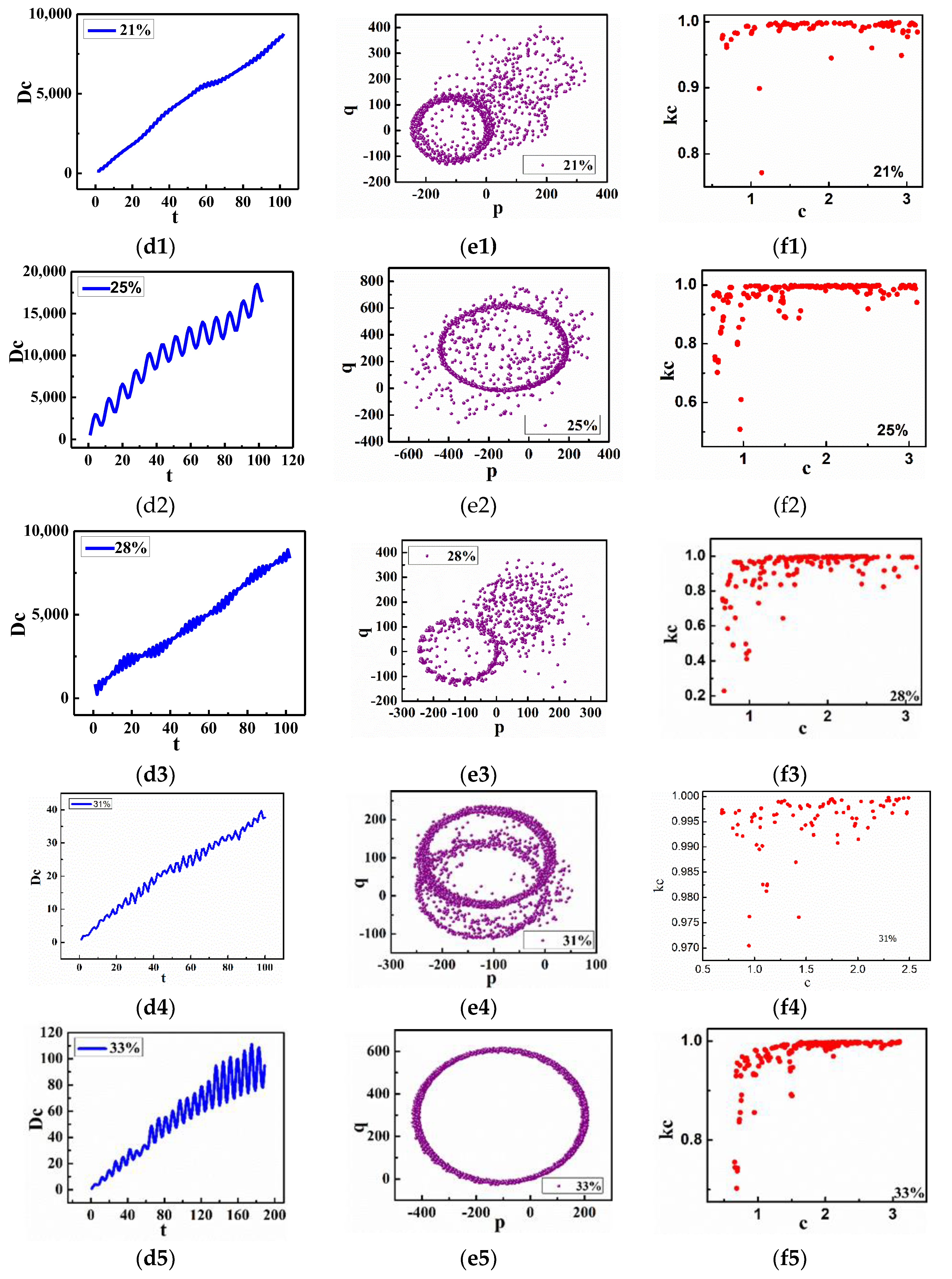
3.4. The 0-1 Test Method

Thinking about the flame image, gray scale time series can reflect the interrelationships among combustion processes. It is applicable to the 0-1 test. Defining the time series as x(j), two additional transfer variables $p\left(n\right)$ and $q\left(n\right)$ can be defined as follows:

$$p\left(n\right)={{\displaystyle \sum }}_{j=1}^{n}x\left(j\right)cos\left(jc\right),n=1,2, \cdots ,N,$$

(3)

and

$$q\left(n\right)={{\displaystyle \sum }}_{j=1}^{n}x\left(j\right)sin\left(jc\right),n=1,2,\cdots ,N,$$

(4)

where n = 1, ⋯, N and c $\in$ [0, π] is a random frequency. However, different c will result in different $p\left(n\right)$ and $q\left(n\right),$ and some values of c will lead to resonance. In order to reduce resonance-causing distortion of results, the constant c is limited to the interval of [π/5,4π/5]. Gottwald and Melbourne suggested the 100 random numbers generated in the section [32,33].

If the discrete time series trajectory of $p\left(n\right)$ and $q\left(n\right)$ approximates Brownian motion, this proves the time series is chaotic.

To determine the growth of $p\left(n\right)$ and $q\left(n\right)$, it is convenient to look at the modified mean square displacement (MSD), defined as $M_c\left(n\right)$, which is the definition of asymptotic properties:

$$M_c\left(n\right)=\underset{N\to \infty }{lim}\frac{1}{N}{\displaystyle \sum }_{j=1}^N\{[p\left(j+n\right)-p{\left(j\right)}^2]+{\left[q\left(j+n\right)-q\left(j\right)\right]}^2\},$$

(5)

where N is the total number of all signal points and n is the magnitude of the time delay for calculating the displacement. From time j to time j + n, the square of the displacement on planes p(n) and q(n) is the term in brackets. $M_c\left(n\right)$ shows the average of all these squared displacements assessed over all time lags of the trajectory. For regular time series $M_c\left(n\right)$ is bounded, while for chaotic time series it increases linearly with time.

There is still a revised least squares displacement, which shows the same asymptotic increase as $M_c\left(n\right)$, but has better convergence quality, defined as D_c(n):

$$D_c\left(n\right)=M_c\left(n\right)-{\left(E\left(\phi \right)\right)}^2\frac{1-\cos \left(nc\right)}{1-\cos \left(c\right)},$$

(6)

where

$${\left(E\left(\phi \right)\right)}^2=\underset{N\to \infty }{\lim }\frac{1}{N}{{\displaystyle \sum }}_{j=1}^{N}x\left(j\right).$$

(7)

The performance of $D_c\left(n\right)$ can also be used to measure the convergence and divergence of $p\left(n\right)$ and $q\left(n\right).$ If the given time series is ordered, $D_c\left(n\right)$ is a bounded quantity; if the given time series is chaotic, $D_c\left(n\right)$ increases linearly with n. For the range of n, $n\le n_{cut}=\frac{N}{10}$ is generally selected. After calculating $M_c\left(n\right)$ or $D_c\left(n\right)$ the index sought is provided by any metric K_c, representing its asymptotic growth rate.

Linear regression and the correlation coefficient are two methods to distinguish K_c.

One way to define chaotic index K_c is as the correlation coefficient between $D_c\left(n\right)$ and linear growth. Linear growth is defined as the ratio between the product of covariance (cov($\xi$, $\eta$)) and standard deviation or variance (var($\xi$)):

$$K_c=\frac{\mathrm{cov}\left(\xi ,\eta \right)}{\sqrt{\mathrm{var}\left(\xi \right)·\mathrm{var}\left(\eta \right)}},$$

(8)

where ξ = 1, 2, $\cdots$, n, $\eta$ = $\left(D_c\left(1\right),D_c\left(2\right),D_c\left(3\right),D_c\left(4\right),\cdots D_c\left(n\right)\right)$. It is commonly believed that the correlation coefficient will be between −1 and 1, and Gottwald and Melbourne proved that the correlation is usually at 0 to 1.

Parameter K provides asymptotic characteristics of $p\left(n\right)$ and $q\left(n\right)$ dynamic systems. However, the value of parameter c will greatly affect the dynamic characteristics of the system. Therefore, different c will produce different K values and resonance phenomena. In order to solve this problem, Gottwald and Melbourne suggested using different c values to repeatedly calculate K values and taking the median of all K_c results as the final index of chaos.

The second way holds that the linear regression method defines a straight line, which is suitable for the logarithmic graph of $D_c$ against n to minimize the square deviation.

This method minimizes the residual error of the linear model:

$$K_c=\underset{n\to \infty }{\lim }\frac{\ln D_c\left(n\right)}{\ln n}.$$

(9)

4. Results and Analysis

Quantitative information is obtained from the average of statistical and spectral parameters, which are calculated on some parts of the registration area.

4.1. Flame Image Feature

Using suitable functions available in MATLAB, the feature vectors described above were calculated for all flame images grabbed during the experimental campaign. In the experiment, pictures were taken from the start of flame ignition: 75 pictures were taken every 10 s, and 1000 pictures were taken continuously. In Figure 3, the 1st (first second), 300th (40th second), 500th (67th second), 800th (108th second), and 1000th (135th second) pictures were respectively selected under oxygen content of 21%, 25%, 28%, 31%, and 33%. The development process of flame could be clearly seen from the evolution rule of flame state in the picture sequence.

In the same combustion time, with increased oxygen content, the burning time of the flame became longer, and its burning area and intensity were also larger. It can be seen from Figure 3 that with increased oxygen content in the combustion-supporting gas, the flame length shows a trend of increasing at the beginning and then decreasing. With increased oxygen content in the combustion-supporting gas, on the one hand, the waste oil biodiesel can be burned more fully; on the other hand, the intensity of combustion is increased, so under the condition of 25% oxygen concentration, the more sufficient combustion of waste oil biodiesel causes a short increase in flame length. With a further increase of oxygen concentration, the intensity of combustion increased, resulting in decreased flame length.

The flame length of waste oil biodiesel combustion fluctuated greatly, and gradually decreased with the increased oxygen content of combustion-supporting gas. Due to the influence of viscosity, the atomization effect of waste oil biodiesel is poor. Inadequate atomization will lead to large-diameter oil droplets. The existence of large-diameter oil droplets will cause the flame length of waste oil combustion to fluctuate greatly. With the increased oxygen content in combustion-supporting gas, the combustion effect of waste oil biodiesel was improved, and the fluctuation degree of flame length gradually decreased. The fluctuation degree of flame luminance was large, and gradually decreased with the increased oxygen content. As the combustion state of the flame in the test was a transition process from carbonization flame to oxidation flame, the luminance of the flame was related to the content of free carbon in the transition stage, and the instability of the content of free carbon causes the luminance to fluctuated greatly. With increased oxygen content, the content of free carbon decreased gradually and the fluctuation degree of flame luminance decreased gradually. With increased oxygen enrichment degree, the proportion of the outer flame increased, and the average gray scale of the whole flame decreased due to the lower gray scale of the outer flame image. When the oxygen enrichment was 21%, the higher average gray scale of the flame was caused by the burning of free carbon contained in the flame to emit bright light spots. However, under other oxygen enrichment conditions, with increased oxygen enrichment, the higher flame luminance was due to higher oxygen concentration and combustion intensity.

4.2. Power Spectrum Analysis of Time Series

A typical frequency domain signal stored by a single pixel is shown in Figure 4. From the five gray scale time series a1 to a5, it was found that the fluctuation range of the flame image gradually tended to be stable with increased oxygen content under the gray scale threshold value of 70, and the time series under the first three working conditions were violently vibrated and decreased; in particular, the gray scale was violently vibrated under the oxygen content of 21%, the surface temperature was very unstable under this working condition, and the combustion was not fully carried out. From the gray scale time series of b1 to b5 species, it could be found that with the continuous advancement of combustion time, the fluctuation of gray scale time series of flame below a threshold value of 170 under the first three working conditions was still very large, the fluctuation amplitude was larger and more severe than in a, and the combustion instability of flame was fully reflected. With the passage of time, under the combustion condition of increasing oxygen enrichment degree, the fluctuation region of flame gray value was stable, and the oscillation amplitude was obviously decreased, which indicates that the high-temperature region of the flame could be maintained for a longer time and the flame could continuously combust more stably.

Images c1 to c5 took the comparison of power maps of two gray scale time series under different oxygen contents. Under working conditions c1, c2, and c3, the power spectrum of the flame gray scale sequence fluctuated obviously, the black line fluctuated more violently, and the peaks and troughs of the two sequences were more dense, with the two time sequences showing overlapping parts. Under conditions c4 and c5, the power spectrum fluctuation amplitude of the time series and the oscillation frequency decreased, which indicates that the combustion stability was further strengthened.

Meanwhile, it can be seen from all the images in Figure 4 that the combustion of the flame was not a periodic change process. The change of oxygen enrichment degree under the initial combustion condition had a significant impact on the combustion effect.

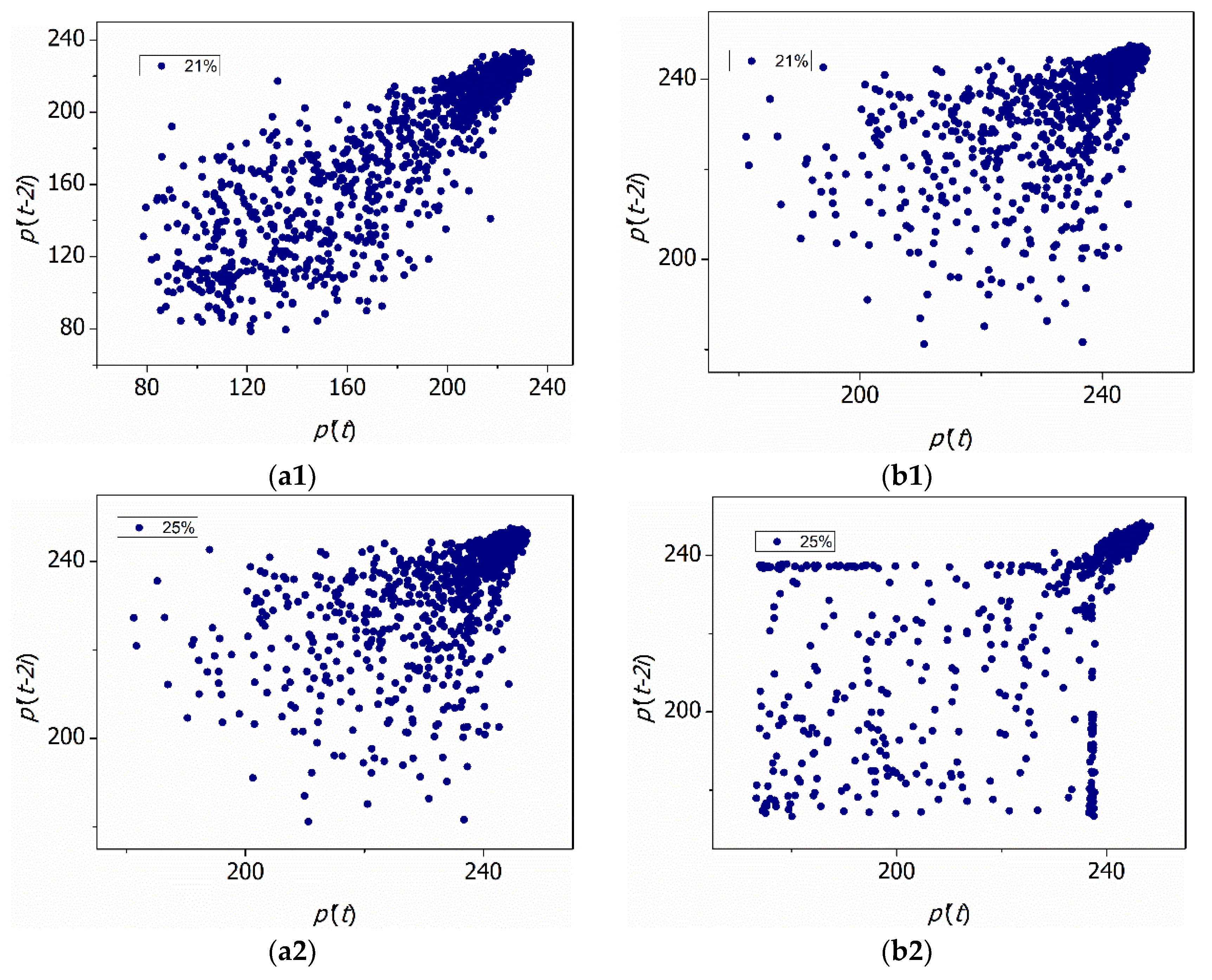
4.3. Phase Reconstruction Method

Figure 5 shows two-dimensional scatter diagrams of flame gray scale time series phase space reconstruction. According to the definition of chaos, it can be seen that under five combustion conditions, the phase points of the time series show a tendency to approach a certain attractor set, which indicates that the gray scale time series showed strong chaotic characteristics in the phase space after the phase space reconstruction. With increased oxygen content, the attraction of the attractor was gradually strengthened, and the distribution of discrete points was gradually concentrated and closed. Especially at 33% oxygen content, the phase points developed and evolved from the above four elongated discrete forms into circular discrete forms. In Figure 5, the images on the left represented the time series under the threshold with gray scale greater than 70, and those on the right represent the time series under the threshold with gray scale greater than 170.

4.4. 0-1 Test Results

Two kinds of threshold analysis were carried out on the flame gray image. One was where the image gray scale was greater than 70, and the image presented at this time was all areas of the flame; the other was where the gray scale was greater than 170, and the high-temperature combustion area of the flame was presented at this time, with brighter luminance. The 0-1 test results are showed in Figure 6 of the gray scale threshold is 70 and Figure 7 of the gray scale threshold is 170. From the calculation rults, it can be seen that with increased oxygen content, the whole flame and its high-temperature region gradually presented strong chaotic characteristics, which shows that with increased oxygen enrichment degree, the combustion effect of the flame was better, the combustion stability was further strengthened, the combustion reaction duration was longer, and the combustion reaction of waste oil biodiesel was more sufficient. The index of judging chaos by the 0-1 test method was mainly to see whether D_c-t is Brownian motion. Under the two thresholds, the movement rule of the time series was from higher divergence to centralized development, which indicates that the fluctuation of the time series was further reduced. Combined with the flame images in a certain period from ignition to full combustion to gradual extinguishment, it can be found that the flame was easier to extinguish and the chaotic characteristics of its high-temperature region were more obvious under the condition of less oxygen enrichment.

However, in the process of using chaos 0-1 to test and calculate, a phenomenon was found. There are two indices for determining chaos: through D_c-t and p-q diagrams, which are used for qualitative analysis, and K_c-c value, used for quantitative analysis. In the calculation process, it was found that the K_c value of the time series was basically close to 1 under the five working conditions, and the K_c value had a wide distribution area under conditions of 25% and 28% oxygen content. After many times of calculation, it could be determined that 40% K_c value was distributed between 0.5 and 0.2, which indicates that at this time, the system was in a weak chaotic state and the p-q trajectory diagram showed a phenomenon from bounded to disordered. With increased oxygen content, the combustion was more complete and K_c value tended to 1 completely. At this time, the system became completely chaotic. A bounded and stable p-q trajectory graph also appeared in the calculation. This was because the calculation of the time series sometimes fluctuated when using the 0-1 chaos test. At this time, the qualitative analysis could no longer meet the discrimination requirements, and we should take the result of the quantitative analysis, namely K_c value, as the standard.

4.5. Calculation Results of the Largest Lyapunov Exponent

In order to verify the feasibility of the 0-1 test, this paper also used the traditional largest Lyapunov exponent (LLE) to analyze the time series. The results are shown in

Table 2. Calculation results of largest Lyapunov exponent (LLE).

Gray Scale	Oxygen Enrichment Concentration
	21%	25%	28%	31%	33%
70	1.3260	1.3187	1.2078	1.7055	1.9866
170	0.9812	0.6193	0.3063	3.0770	2.8896

. After calculating the gray scale time series of the flame images under the two thresholds, all LLEs were positive, which shows that the system was chaotic and the feasibility of the 0-1 test is verified once again.

When the gray threshold value was 70, the LLEs of the five working conditions were between 1 and 2, without obvious oscillation and fluctuation. This shows that the increased oxygen content would not significantly affect the distribution of the whole flame area from the overall distribution of the flame, but the chaotic trend became more obvious. When the oxygen content was 33%, the gray scale time series had strong chaotic characteristics.

When the gray scale threshold was 170, the main research at this time was the combustion situation in the high-temperature region of the flame. It could be seen that with increased oxygen content in the combustion-supporting air, the high-temperature combustion distribution of the flame showed strong chaotic characteristics after 30%, indicating that the combustion effect of the flame was the best at this time.

5. Conclusions

(1) According to the test results, it was found that different oxygen concentrations had a great influence on the combustion strength and stability of waste oil biodiesel. In this paper, the common flame gray scale in flame image processing was taken as the research index. Under the stable combustion condition, the average gray value of the image was maintained at a high level and fluctuates slightly up and down. During unstable combustion, the average gray value of the image was lower than that of the stable combustion condition. When the fluctuation range was large and flameout occurred, the average gray value of the image rapidly dropped extremely low.

(2) Using common methods to judge the chaotic characteristics of time series (phase space reconstruction, largest Lyapunov exponent, power spectrum, and the 0-1 chaotic test), flame gray scale time series under different thresholds were calculated and analyzed. The results show that all gray scale distributions of the flame showed chaotic characteristics for the oxygen-enriched combustion of waste oil biodiesel. With gradually increasing oxygen content, the flame showed more intense chaotic characteristics, and all kinds of discrimination indices showed strong chaotic characteristics.

(3) The nonlinear characteristics of the biodiesel oxygen-enriched combustion system showed a gradual transition from quasi-periodic to chaotic, and the high-temperature combustion area was gradually expanded and strengthened. This shows that the combustion system became more complex and more chaotic and the combustion effect was improved after the oxygen-enriched combustion method was applied. The increased oxygen enrichment degree induced a gradual transition from unstable to stable for stable and efficient combustion of the flame. When the oxygen content reached 33%, the combustion effect of the flame was the best in all test conditions. After calculation, it was found that the oxygen enrichment degree and chaotic K_c correlation coefficient were 0.88 and 0.86 respectively under two groups of gray scale time series. Which indicate that with the increase of oxygen content, the chaotic intensity was gradually increasing and the combustion effect was getting better and better.

References

1. Aransiola, E.F.; Ojumu, T.V.; Oyekola, O.O.; Madzimbamuto, T.F.; Ikhu-Omoregbe, D.I.O. A review of current technology for biodiesel production: State of the art. Biomass Bioenerg. 2013, 61, 276–297. [Google Scholar] [CrossRef]
2. Ashraful, A.M.; Masjuki, H.H.; Kalam, M.A.; Rizwanul Fattah, I.M.; Imtenan, S.; Shahir, S.A.; Mobarak, H.M. Production and comparison of fuel properties, engine performance, and emission characteristics of biodiesel from various non-edible vegetable oils: A review. Energy Conversi. Manag. 2014, 80, 202–228. [Google Scholar] [CrossRef]
3. Reddy, V.M.; Biswas, P.; Garg, P.; Kumar, S. Combustion characteristics of biodiesel fuel in high recirculation conditions. Fuel Process. Technol. 2014, 118, 310–317. [Google Scholar] [CrossRef]
4. Docquier, N.; Sébastien, C. Combustion control and sensors: A review. Prog. Energy Combust. Sci. 2002, 28, 107–150. [Google Scholar] [CrossRef]
5. Ballester, J.; Tatiana, G.-A. Diagnostic techniques for the monitoring and control of practical flames. Prog. Energy Combust. Sci. 2010, 36, 375–411. [Google Scholar] [CrossRef]
6. Zhang, C. Study on Combustion Characteristics of Biodiesel in Furnace; Central South University: Hunan, China, 2012. [Google Scholar] [CrossRef]
7. Wang, C. Study on the Influence of Air Preheating Temperature on Combustion Characteristics of Biodiesel; Central South University: Hunan, China, 2013. [Google Scholar] [CrossRef]
8. Jiang, Y.; Jiang, S.; Huang, L.; Chen, L.; Zhong, W. Experimental Study on Temperature Field of Biodiesel Combustion Flame. J. Cent. South Univ. (Nat. Sci. Ed.) 2015, 46, 540–3545. [Google Scholar] [CrossRef]
9. Jiang, S.; Zhong, W.; Zhang, C.; Wang, C. Study on Flame Characteristics of Biodiesel in Furnace Based on Image Processing Technology. J. Agric. Mach. 2013, 44, 24–29. [Google Scholar] [CrossRef]
10. Ibrahim, A. Performance and combustion characteristics of a diesel engine fuelled by butanol–biodiesel–diesel blends. Appl. Therm. Eng. 2016, 103, 651–659. [Google Scholar] [CrossRef]
11. Calder, J.; Roy, M.M.; Wang, W. Performance and emissions of a diesel engine fueled by biodiesel-diesel blends with recycled expanded polystyrene and fuel stabilizing additive. Energy 2018, 149, 204–212. [Google Scholar] [CrossRef]
12. Qubeissi, A.M. Predictions of droplet heating and evaporation: An application to biodiesel, diesel, gasoline and blended fuels. Appl. Therm. Eng. 2018, 136, 260–267. [Google Scholar] [CrossRef]
13. Kilic, G.; Sungur, B.; Topaloglu, B.; Ozcan, H. Experimental analysis on the performance and emissions of diesel/butanol/biodiesel blended fuels in a flame tube boiler. Appl. Therm. Eng. 2018, 130, 195–202. [Google Scholar] [CrossRef]
14. Jeon, J.; Park, S. Effect of injection pressure on soot formation/oxidation characteristics using a two-color photometric method in a compression-ignition engine fueled with biodiesel blend (B20). Appl. Therm. Eng. 2018, 131, 284–294. [Google Scholar] [CrossRef]
15. Lei, S.; Turan, A. Nonlinear/Chaotic Modeling and Control of Combustion Instabilities. Int. J. Bifurc. Chaos 2010, 20, 1245–1254. [Google Scholar] [CrossRef]
16. Margolis, S.B. Chaotic combustion of solids and high-density fluids near points of strong resonance. Proceedings of the Royal Society A: Mathematical. Phys. Eng. Sci. 1991, 433, 131–150. [Google Scholar] [CrossRef]
17. Lei, S.; Turan, A. Chaotic modelling and control of combustion instabilities due to vaporization. Int. J. Heat Mass Transf. 2010, 53, 4482–4494. [Google Scholar] [CrossRef]
18. Ferrante, L.; Miccio, M.; Miccio, F.; Solimene, R. Fluidized Bed Combustion of Liquid Biofuels: Application of Integrated Diagnostics for Micro-explosions Characterization. Energy Fuels 2008, 22, 4213–4222. [Google Scholar] [CrossRef]
19. Kuzmych, O.; Aitouche, A.; El Hajjaji, A.; Bosche, J. Nonlinear control for a diesel engine: A CLF-based approach. Int. J. Appl. Math. Comput. Sci. 2014, 24, 821–835. [Google Scholar] [CrossRef]
20. Wang, L.Y.; Yang, L.P.; Ma, X.Z.; Li, J. Analysis of chaos combustion process in spark ignition natural gas engine. J. Beijing Univ. Technol. 2012, 38, 689–964. [Google Scholar]
21. Lorenz, E.N. Deterministic nonperiodic flow. J. Atmos. Sci. 2004, 20, 130–141. [Google Scholar] [CrossRef]
22. Rand, D.A.; Young, L.S. Dynamical systems and turbulence, Warwick 1980; Springer: New York, NY, USA, 1981. [Google Scholar] [CrossRef]
23. Grassberger, P.; Procaccia, I. Characterization of Strange Attractors. Phys. Rev. Lett. 1983, 50, 346–349. [Google Scholar] [CrossRef]
24. Packard, N.H.; Crutchfield, J.P.; Farmer, J.D.; Shaw, R.S. Geometry from a time series. Phys. Rev. Lett. 2008, 45, 712. [Google Scholar] [CrossRef]
25. Wolf, A.; Swift, J.B.; Swinney, H.L.; Vastano, J.A. Determining Lyapunov exponents from a time series. Phys. D Nonlinear Phenom. 1985, 16, 285–317. [Google Scholar] [CrossRef]
26. Sano, M.; Sawada, Y. Measurement of the Lyapunov Spectrum from a Chaotic Time Series. Phys. Rev. Lett. 1985, 55, 1082–1085. [Google Scholar] [CrossRef]
27. Cheng, M.-Y.; Prayogo, D.; Ju, Y.-H.; Wu, Y.-W.; Sutanto, S. Optimizing Mixture Properties of Biodiesel Production Using Genetic Algorithm-Based Evolutionary Support Vector Machine. Int. J. Green Energy 2016, 13, 1599–1607. [Google Scholar] [CrossRef]
28. Saurabh, A.; Kabiraj, L.; Wahi, P.; Sujith, R.I. Route to chaos for combustion instability in ducted laminar premixed flames. Chaos Interdiscip. J. Nonlinear Sci. 2012, 22, 23129. [Google Scholar]
29. Maheshwari, N.; Balaji, C.; Ramesh, A. A nonlinear regression based multi-objective optimization of parameters based on experimental data from an IC engine fueled with biodiesel blends. Biomass-Bioenergy 2011, 35, 2171–2183. [Google Scholar] [CrossRef]
30. Davies, M.L.; Halford-Maw, P.A.; Hill, J.; Tinsley, M.R.; Johnson, B.R.; Scott, S.K.; Kiss, I.Z.; Gaspar, V.; Kiss, I. Control of Chaos in Combustion Reactions. J. Phys. Chem. A 2000, 104, 9944–9952. [Google Scholar] [CrossRef]
31. Gotoda, H.; Nikimoto, H.; Miyano, T.; Tachibana, S. Dynamic properties of combustion instability in a lean premixed gas-turbine combustor. Chaos: Interdiscip. J. Nonlinear Sci. 2011, 21, 13124. [Google Scholar] [CrossRef]
32. Gottwald, G.A.; Melbourne, I. On the implementation of the 0-1 test for chaos. SIAM J. Appl. Dyn. Syst. 2009, 8, 129–145. [Google Scholar] [CrossRef]
33. Gottwald, G.A.; Melbourne, I. On the validity of the 0-1 test for chaos. Nonlinearity 2009, 22, 1367–1382. [Google Scholar] [CrossRef]
34. Ding, S.-L.; Song, E.-Z.; Yang, L.-P.; Litak, G.; Yao, C.; Ma, X.-Z. Investigation on nonlinear dynamic characteristics of combustion instability in the lean-burn premixed natural gas engine. Chaos Solitons Fractals 2016, 93, 99–110. [Google Scholar] [CrossRef]
35. Ding, S.-L.; Song, E.-Z.; Yang, L.-P.; Litak, G.; Wang, Y.-Y.; Yao, C.; Ma, X.-Z. Analysis of chaos in the combustion process of premixed natural gas engine. Appl. Therm. Eng. 2017, 121, 768–778. [Google Scholar] [CrossRef]
36. Liping, Y.; Xiuzhen, M.; Enzhe, S. Influence of Mixture Quality on Nonlinear Combustion Process of Natural Gas Engine. In Proceedings of the International Conference on Intelligent System Design & Engineering Application (IEEE), Changsha, China, 13–14 October 2010. [Google Scholar] [CrossRef]
37. Dong, Z.; Liu, M. Intelligent Diagnosis Method of High Temperature and Low Oxygen Flame Images; Electronic Industry Press: Beijing, China, 2012; pp. 40–100. [Google Scholar]
38. Yang, W.; Blasiak, W. Chemical Flame Length and Volume in Liquified Propane Gas Combustion Using High-Temperature and Low-Oxygen-Concentration Oxidizer. Energy & Fuels 2004, 18, 1329–1335. [Google Scholar]
39. Fleury, A.; Trigo, F.; Pacífico, A.; Martins, F. An inference model for combustion diagnostics in an experimental oil furnace. Expert Syst. 2017, 35, e12245. [Google Scholar] [CrossRef]
40. Hernandez, R.; Ballester, J. Flame imaging as a diagnostic tool for industrial combustion. Combust. Flame 2008, 155, 509–528. [Google Scholar] [CrossRef]
Figure 1. Schematic diagram of spray nozzle structure.
Energies 12 04479 g001
Figure 2. Flame monitoring system located in the combustion chamber.
Energies 12 04479 g002
Figure 3. Flame combustion image sequence under different oxygen contents.
Energies 12 04479 g003
Figure 4. Gray scale time series with different thresholds and their power spectra: time series when gray scale threshold is (a1a5) 70 and (b1b5) 170, and (c1c5) power spectra of two time series.
Energies 12 04479 g004aEnergies 12 04479 g004b
Figure 5. Reconstruction of 2-D scatter diagrams from time series phase space for flame images with different oxygen content at (a1a5), 70 gray scale threshold and (b1b5), 170 gray scale threshold.
Energies 12 04479 g005aEnergies 12 04479 g005b
Figure 6. Results of the 0-1 test with gray scale threshold of 70: (a1a5) Dc-t phase diagram, (b1b5), p-q phase diagram, and (c1c5), Kc-c phase diagram.
Energies 12 04479 g006
Figure 7. Results of the 0-1 test with a gray scale threshold of 170: (d1d5) Dc-t phase diagram, (e1e5) p-q phase diagram, and (f1f5) Kc-c phase diagram.
Energies 12 04479 g007