Article

Comparison of the Greenhouse Gas Emission Reduction Potential of Energy Communities

1
Copernicus Institute of Sustainable Development, Utrecht University, Princetonlaan 8a, 3584 CB Utrecht, The Netherlands
2
Institute for Renewable Energy, Eurac Research, Viale Druso 1, 39100 Bolzano, Italy
*
Author to whom correspondence should be addressed.
These authors contributed equally to this work.
Energies 2019, 12(23), 4440; https://doi.org/10.3390/en12234440
Submission received: 12 October 2019 / Revised: 14 November 2019 / Accepted: 19 November 2019 / Published: 22 November 2019
(This article belongs to the Special Issue Assessment of Photovoltaic-Battery Systems)

Abstract

:
In this research, the greenhouse gas (GHG) emission reduction potentials of electric vehicles, heat pumps, photovoltaic (PV) systems and batteries were determined in eight different countries: Austria, Belgium, France, Germany, Italy, the Netherlands, Portugal and Spain. Also, the difference between using prosuming electricity as a community (i.e., energy sharing) and prosuming it as an individual household was calculated. Results show that all investigated technologies have substantial GHG emission reduction potential. A strong moderating factor is the existing electricity generation mix of a country: the GHG emission reduction potential is highest in countries that currently have high hourly emission factors. GHG emission reduction potentials are highest in southern Europe (Portugal, Spain, Italy) and lowest in countries with a high share of nuclear energy (Belgium, France). Hence, from a European GHG emission reduction perspective, it has most impact to install PV in countries that currently have a fossil-fueled electricity mix and/or have high solar irradiation. Lastly, we have seen that energy sharing leads to an increased GHG emission reduction potential in all countries, because it leads to higher PV capacities.

Graphical Abstract

1. Introduction

European Union (EU) strategies for a low carbon built environment include the electrification of heating systems in buildings through heat pumps [1], and electrification of transport which combines vehicles with efficient powertrains and the opportunity of using renewable energy sources (RES) [2]. Currently, heat pumps account for 5% in sales for heating requirement and 3% in energy for heating. However, in the International Energy Agency scenarios towards a sustainable future, heat pumps make up from 10% to 30% of the heating equipment stock [3]. At the same time, the global EV fleet has shown a large expansion in recent years, from 1.3 million EVs in 2015 to 5.1 million EVs in 2018 [3], and this development will only be intensified since electric light duty vehicles are expected to reach cost parity with internal combustion engine vehicles (ICEVs) around 2025 in many major markets, driven mainly by declining battery costs [4]. PV technology has evolved in the past decades into a major renewable electricity supplying technology with a total installed capacity of 600 GW [5]. As a result of the large deployment of PV systems, there is an ongoing transition from centralized to decentralized electricity generation. Hence, the role of residential consumers on the electricity market is changing, from being solely consumers of electricity, to becoming so-called prosumers, i.e., both producing and consuming electricity [6].
The integration of electric vehicles and heat pumps into the electricity system provides opportunities but also poses challenges. Both technologies are synergistic with renewable energy sources, and especially PV generation, in terms of a primary renewable energy input and increased self-consumption [7,8]. However, the electrification of heating and transport systems also poses challenges to the electricity grid, since heating and charging requirements often coincide with peak electricity demand hours. Staffell and Pfenninger (2018) found that heat supply electrification could increase peak electricity demand in the UK by 20% within 15 years [9], whereas another study found that a 50% penetration rate of heat pumps can result into an increase of 27.5% in peak electricity demand in the UK [10]. Similarly, in the case of uncontrolled charging, the EV charging demand can lead to congestion problems, high capacity reinforcement investment needs and less efficient power supply [11,12,13]. To enable an effective transition to an electrified and sustainable energy system, the concepts of electricity storage, smart grids, and demand response are getting increased attention. Especially, battery energy storage systems (BESS) are expanding fast, with the aim of providing short-term storage. A BESS can improve the efficiency of the power system by providing additional flexibility to grid operators, such as the provision of ancillary services, peak shaving, congestion management and reduction of reserve provision from conventional units [14,15,16]. Battery storage capacity is growing fast, actually tripled in less than three years, largely driven by lithium ion batteries, which now account for just over 80% of all battery capacity [4]. In this context, photovoltaic (PV) systems, battery-electric vehicles (BEVs), BESS, and heat pumps (HPs) are key technologies in decarbonising cities. However, this development will require integration technologies such as smart grids and ICT to enable a seamless operation.
The term “smart grid” generally refers to an electricity grid which uses information and communication technologies tools to balance electricity demand and generation, taking into account the intermittent nature of RES, demand side management (DSM) and electricity storage [17]. The main aim of smart grids is to ensure cost-optimal use of RES electricity while minimizing the need for grid re-enforcement due to the strong increases in electricity demand and intermittent decentralized generation. The research on smart grids also includes the concepts of energy communities or energy sharing [18]. An energy community can be broadly defined as a group of consumers and/or prosumers, that together share energy generation units and electricity storage. The idea is that it is financially beneficial to exchange energy within this community, rather that exchanging it with the grid. This would decrease requirements for grid re-enforcement, and thus allow for a larger deployment of RES (such as PV systems) in urban environments.
To analyze different business cases for PV prosumers, taking into account electricity storage, BEVs and other technologies, the EU-funded PVP4Grid project was initiated [19]. The main project aim is to increase the market share and value of PV, by enabling consumers to become prosumers, in a system-friendly manner. Among other activities, the project has analyzed different grid concepts or scenarios: (1) consumers purchasing electricity individually from the grid, (2) consumers purchasing and producing electricity individually (with the possibility to invest in PV and/or BESS), and (3) consumers forming energy communities, together optimizing purchasing electricity and investments in PV and BESS. The objective is to show how the overall costs for consumers change, and what the benefits are of forming energy communities. The results indicate that investments in BESS and especially PV systems are more than offset by savings in electricity purchase, and that these benefits are further increased when forming energy communities [20].
Next to financial considerations, environmental concerns also play an important role in investments decisions of homeowners [21]. Furthermore, an important underlying rationale of offering incentives for decentralized renewable electricity generation is the mitigation of greenhouse gas (GHG) emissions. Therefore, in this study an assessment is performed on the GHG emission reduction potential of various decentralized energy technologies of a reference European community, taking their full life cycle into account. The focus in this paper is on technologies that enable the electrification of heating and transport systems. As explained above, EV and HP technologies are key in decarbonizing cities, and at a state of technological development that result into growing market shares worldwide. However, electrification will only be viable if power generation is decarbonized in parallel [22], and supported by grid integration measures. To further increase the comprehensiveness of the GHG impact assessment, it is performed for eight different countries: Austria, Belgium, France, Germany, Italy, the Netherlands, Portugal and Spain. These eight countries are the target countries defined in the PVP4Grid project and they provide a comprehensive selection from Southern, Western and Central Europe in terms of climate and generation mix. In this way, it can be determined in which countries the prosumer concepts have the highest climate mitigation potential.
Since the electrification of heating and transport is primarily aimed at reducing GHG emissions, numerous authors have performed life-cycle assessments (LCAs) of these technologies, to establish a.o. their GHG reduction potentials. Of the technologies considered here, PV systems likely have the longest history of LCA studies, with first examples of somewhat basic LCA studies dating back roughly forty years [23,24]. Since the publication of those early works, the field of LCA has developed significantly, with many analyses of PV modules and systems (see e.g., a comprehensive review in [25]), and renewable energy technologies in general have been thoroughly studied [26,27]. For all technologies studied here, a large number of LCA studies are available. Many publications focus on the manufacturing of the technologies, but additionally, publications are available that also include or even focus on the use-phase.
For BEVs, most commonly a comparison is made for passenger vehicles, focusing on a comparison between traditional ICEVs vs. BEVs or plug-in hybrid-electric vehicles (PHEVs), hence the results are expressed as environmental impact per passenger-kilometer [28,29,30,31,32,33,34,35]. Also for heatpumps, LCAs conducted often make a comparisong between the novel technology and its incumbent competitor, which is in the case of heating mostly a natural gas fired boiler [36,37,38,39,40,41,42,43]. LCAs of battery storage systems are much less widespread, as was discussed by Pellow et al. [44], especially those including use-phase impacts. For all technologies mentioned here, the use-phase makes a substantial contribution to the overall life-cycle environmental impact. Since the increased attention for the concept of decarbonistation of the built environment, several LCAs have also been conducted that analyse e.g., zero-energy buildings or even neighborhoods and micro-grids [45,46,47].
In traditional LCA approaches, average emission factors (AEFs) are used to reflect the GHG intensity to account for the electricity consumption during the lifetime of a technology. This implicitly assumes emission factors are constant during the year. In reality, emission factors fluctuate during the season and the day because of variable renewable electricity generation, which have low emission factors, and as a result of the economic dispatch of conventional technologies, which have large individual differences in GHG intensity [48]. In a future energy system with a very high share of RES, the demand even has to adjust to the electricity supply of variable renewable electricity generation, i.e., DSM. This stresses the importance of using time-varying emission factors instead of AEFs. For most of the LCA studies mentioned above, AEFs were used, with the exception of two studies focusing on the application of batteries [49,50]. Time-varying emission factors have also been used to more accurately determine the impact of energy efficiency measures [51,52] and for deployment of wind power [53], but never in a such comprehensive manner as in our study. As part of this study, the hourly emission factors (HEFs) of the eight aforementioned countries are determined for the year 2017 and used to determine the scope 2 emissions (i.e., emissions related to the use of electricity) of the prosumer concepts.
The contribution of this study is threefold. First, different policy scenarios are compared, quantifying the climate impact of different policy options. Second, eight European countries are compared, which provides insight in how differences between countries influence the GHG mitigation potential of a technology, and simultaneously gives a practical indication of where prosumer concepts have the largest mitigation potential. Third, hourly emission profiles are constructed and the impact of their use is assessed. This is an improvement to current LCA methodology, and moreover the emission profiles are added as Supplementary Materials to enable their use by other scholars and practitioners.
The paper is further structured as follows. In Section 2, all used methods are explained. Section 3, the Results section, is divided into four parts. First, the HEFs are presented. Then, the GHG emissions of the European Communities are compared. Subsequently, GHG impact of individual technologies will be compared per country. Lastly, the impact of using HEFs, as opposed to AEFs, is examined. The paper concludes with the discussion and conclusions in Section 4.

2. Materials and Methods

2.1. Goal and Scope

The typical EU community has been defined in [20] and is shown in Figure 1. This all-electric community consisted of four single housing units, two stand-alone commercial consumers and one apartment building that consisted of one commercial consumer and six apartments. In total, 23 people lived in this community, and they owned a total of 11 BEVs. All rooftops had potential for PV, and heating was supplied by HPs. Also, there was space available for installing one central battery.
Three scenarios were defined: Baseline scenario, the All-electric–No sharing scenario and the All-electric–Sharing scenario. The Baseline scenario entailed one metering point per household and no investment options in PV or BESS. In this scenario, the transport need was assumed to be met by ICEVs and heating was supplied by largely fossil fuel-based heating (see Section 2.3.3). The All-electric–No sharing also entailed individual metering points, but with investment options in PV and BESS. Lastly, the All-electric–Sharing scenario entailed possibility for investment and one central metering point (i.e., energy sharing is allowed). Both the All-electric scenarios had HPs and BEVs deployed. The economic optimization in [20] determined the final configuration of installed PV and BESS capacity. This differed per country because of difference in household electricity profiles, solar irradation and national policies. To calculate the GHG emissions, life-cycle emissions of the aforementioned technologies were taken into account, as well as the household electricity consumption. Construction and decommissioning of the buildings themselves and of other household appliances were outside of the scope of this research. The year of focus was 2017.

2.2. Hourly Emissions Factors

In general, an emission factor can be defined as emissions G H G over an amount of Energy E. For the HEFs, a distinction can be made between the HEFs of electricity generated in a country and the HEFs of electricity consumed in a country. The H E F gen of country j in hour t can be calculated according to Equation (1a,b):
G H G gen , j t = k = 1 K E gen , j k t E F j k
H E F gen , j t = G H G g e n , j t k = 1 K E gen , j k t
where EF is the Emission Factor of generator k ( 1 , 2 , K ) . For the EF of a generator, the weighted average of generators with the specific fuel type in the accordant country was taken from the ecoinvent v3 database [54]. When calculating this weighted average E F , we accounted for the annual generation from different types of generators within each fuel type (e.g., combined cycle vs. conventional generators).
A shortcoming of taking the H E F gen to account for GHG emissions of electricity consumption, is that it neglects import and export of electricity. In reality, electricity consumed is a mixture of electricity generated in a country j and electricity imported from country l ( 1 , 2 , L ) with L being the number of countries that country j has interconnection lines with. So as an intermediate step, the HEF on the high-voltage (HV) lines of a country is be calculated according to Equation (2a,b):
G H G HV , j t = G H G gen , j t + l = 1 L E import , j t l H E F gen , t l
H E F HV , j t = G H G HV , j t E gen , j t + l = 1 L E import , j l t
For countries that were the focus of this study, the H E F gen calculated in Equation (1b) was taken, for other countries the AEF was used from ecoinvent. This resulting mix was exported to neighbouring countries l. So finally, the H E F cons was calculated by using Equation (3a,b):
G H G cons , j t = G H G HV , j t l = 1 L E export , j l t H E F HV , j t
H E F cons , j t = G H G cons , j t E gen , j t + l = 1 L E import , j l t E export , j l t
Electricity generation data were taken from ENTSO-E [55], which reports the hourly generation per fuel type for the EU28 member states. The fuel types encompass Biomass, Fossil Brown Coal/Lignite, Fossil Coal-derived gas, Fossil Gas, Fossil Hard Coal, Fossil Oil, Fossil shale Oil, Fossil Peat, Geothermal, Hydro (pumped, Run-of-river and Water Reservoir), Marine, Nuclear, Solar, Waste, Wind Offshore and Wind Onshore. The treatment of missing data can be found in Appendix A.

2.3. GHG Emissions of Applied Technologies

To account for a shift in technologies, from a scenario with traditional space heating, ICEVs and without any installed PV capacity towards a scenario with HPs for space heating, BEVs and installed PV and BESS, we took into account the GHG emissions related to manufacturing of all mentioned technologies. Using data from the ecoinvent v3 database, we expressed the GHG emissions released during manufacturing in functional units that allowed us to calculate annual GHG emissions attributed to manufacturing of the selected technologies. In Section 2.3.1, Section 2.3.2 and Section 2.3.3 we describe in more detail the underlying data and assumptions made to select the appropriate input data.

2.3.1. Manufacturing of PV and BESS

In the all-electric technology scenarios, investments in PV and BESS were made. To assess the effect that these investments have on annual emissions, we took into account the GHG emissions from manufacturing of these technologies.
For PV systems, we assumed the installation of multi-crystalline, roof-mounted PV systems. Here, we distinguished between flat-roof mounted systems for the apartment and commercial buildings, and slanted-roof systems for the three detached houses (all shown in Figure 1). We chose multi-crystalline systems as these currently have lowest installed system cost, hence they would be the optimal choice in a cost-optimization exercise.
It must be noted that the data in ecoinvent v3 for PV systems is outdated, hence the emissions associated with manufacturing of these systems are much higher than they would be for modern PV systems. However, as we discussed in Section 2.1, we wanted to base all results on LCA data from a single database for consistency between different technologies.
However, for BESS there is unfortunately no complete dataset available in ecoinvent v3 that includes both the battery cells as well as the energy management system and inverter. Hence, for BESS, we based our results on data presented in [8] for the storage and balance-of-system components of BESS. In this study, we assumed a battery C-rate of 0.5, which is in line with most currently commercially available BESS.

2.3.2. Manufacturing of ICEVs and BEVs

To account for the annual emissions related to the operation of passenger vehicles, we compared conventional ICEVs in the baseline scenario with BEVs in the full-electric scenarios. The GHG emissions of both were modelled based on data in ecoinvent v3. This database includes LCA data for a large variety of ICEVs of different sizes and fuel types. For BEVs, there is only one type of passenger vehicle in ecoinvent. For this study, we compared medium EURO5 passenger cars with this single type of BEV. To account for fuel type, we used data from Eurostat [56], which describes the share of diesel vs. petrol engine cars. For Italy we assumed the shares to be the weighted averages of the seven other countries since there were no data available for Italy in the Eurostat dataset.
Since the data from ecoinvent include both the manufacturing of the vehicles, as well as the energy use while driving, we corrected the data for BEVs to exclude electricity use, since the emissions from charging the BEVs were modelled separately.

2.3.3. GHG Emissions Related to Heat Supply

In the baseline scenarios, GHG emissions related to space heating and hot water demand were modelled based on the current shares of different heating technologies in the eight target countries. The Heat Roadmap Europe 4 project published a dataset in 2015 [57] detailing the heating and hot water technologies in several European countries, including our eight target countries. Using these shares, we calculated an average emissions factor for each unit of heat demand (gCO 2 -eq/MJ th ), using as input country specific emissions factors from ecoinvent for each of the heating technologies.
For the all-electric scenarios, we assumed all heat (and hot water) demand to be fulfilled by means of air source HPs. Since the electricity use of the HPs were modelled separately, emissions related to the electricity use of HPs were calculated directly by using the HEFs. Emissions related to manufacturing of the HPs were modelled based on data from ecoinvent v3 that expresses the impact of manufacturing and other auxiliary processes per MJ of heat demand.

2.4. Community-Level GHG Emissions

Using the HEFs, the time series of electricity flows to and from the grid and within the community, and the emissions related to manufacturing of the selected technologies, we calculated the annual emissions for each building in the community, and for the community as a whole. Broadly speaking, GHG emissions in our study can be attributed to:
  • Electricity consumption from the grid
  • Fuel combustion in ICEVs in the baseline scenario
  • Fuel combustion for heating in the baseline scenario
  • Manufacturing of vehicles, PV and battery systems, and heating technologies
  • Electricity feed-in to the grid from PV (avoided or “negative” emissions)
The GHG emissions from grid electricity consumption were calculated by multiplying the two time series of H E F con and grid electricity consumption E G 2 L :
G H G grid , t = H E F con , t · E grid , t
Similarly the emissions avoided by feed-in of PV electricity to the grid were calculated by multiplying the time series of H E F con and PV grid feed-in E PV feed in . The emissions for fuel combustion for car transport and heating, were calculated by multiplying the annual driven kilometers and annual heat demand by the emission factors for transport ( E F car , in gCO 2 -eq per passenger·km) and heating ( E F heat , in gCO 2 -eq/MJ th ), respectively. These emissions factors, taken from ecoinvent v3, also include the GHG impacts of manufacturing the respective technologies.
In the all-electric scenarios, heating and car transport are obviously fully electrified, hence there was no direct fuel combustion. In these scenarios, we attributed the emissions to each process by taking into account the time series of BEV charging and HP electricity demand. Since we modeled the impacts of electricity use for these processes directly, the emission factors E F car and E F heat in this case only included the impacts related to manufacturing. Additionally, in the all-electric scenarios PV systems were installed, hence the emission factors attributed to BEV charging and heat-pump demand were corrected for the share of PV electricity in the overall household electricity demand. Hence, if the complete electricity demand at time t was met by PV electricity, the emission factor at time t for electricity use was 0 gCO 2 -eq/kWh.

2.5. Input Data

The results from the economic optimization from Fleischhacker et al. [20] can be found in Table 1. As mentioned above, these results were the result of national policies, country-specific solar irradiation and the country-specific electricity profiles. These numbers were taken as input for calculating the GHG emissions reduction potential, together with the timeseries of electricity demand from [20]. The study of Fleischhacker et al. analyzed the electricity flows from and to the grid, battery, BEV, HP and PV systems, for the eight target countries, and for each of the building units as shown in Figure 1.
As mentioned above, the generation data per fuel type were taken from [55]. This is a database where individual Transmission System Operators (TSOs), associated in ENTSO-E, upload the hourly load values per production type of the individual countries.
The life-cycle emissions of the technologies as well as the AEFs of countries outside of the scope of this study are taken from ecoinvent v3 [54]. This is a highly regarded, comprehensive life-cycle inventory (LCI) database with LCI data on a vast amount of processes, materials and energy flows.
The time series of the heat demand, electricity demand and BEV charging demand were supplied by the individual country members of the PVP4Grid project. The PV generation time series and battery charging and discharging profiles were a result of a combination of the data supply of the individual countries in the PVP4Grid project and the model results of [20].

3. Results

The results consist of four parts. First, the HEFs are analyzed. Second, the absolute emissions of the previously defined typical European communities are analyzed. This provides insight into the GHG emission reduction potential that of current national policies, as well as the impact of allowing energy sharing. Third, the normalized GHG emission reduction potential are shown for the eight target countries. This provides insight into which technologies have most impact in which location. Lastly, we elaborate on the difference between using AEFs and HEFs. This shows what technologies consume or produce, and times with high or low emission factors.

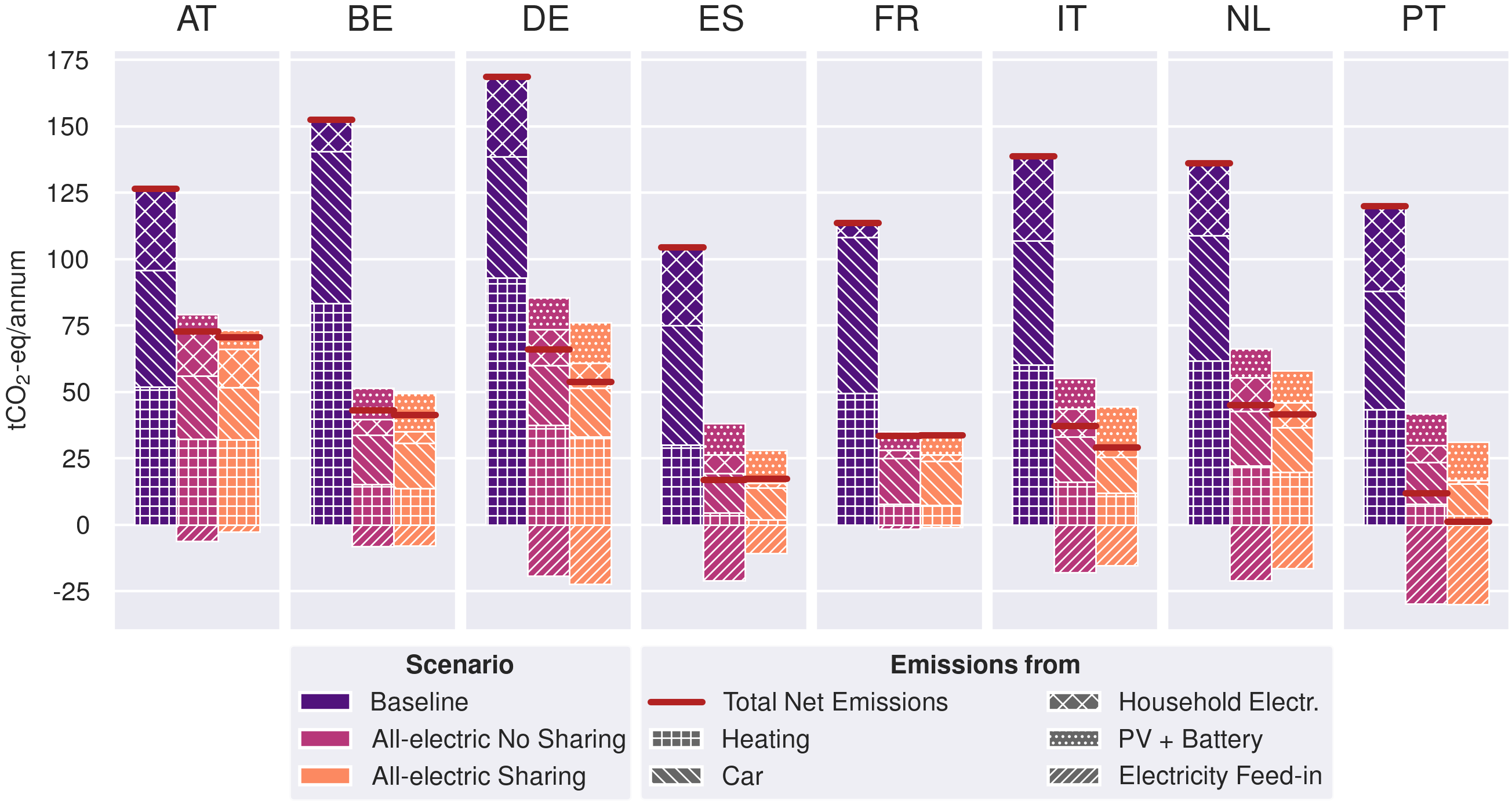
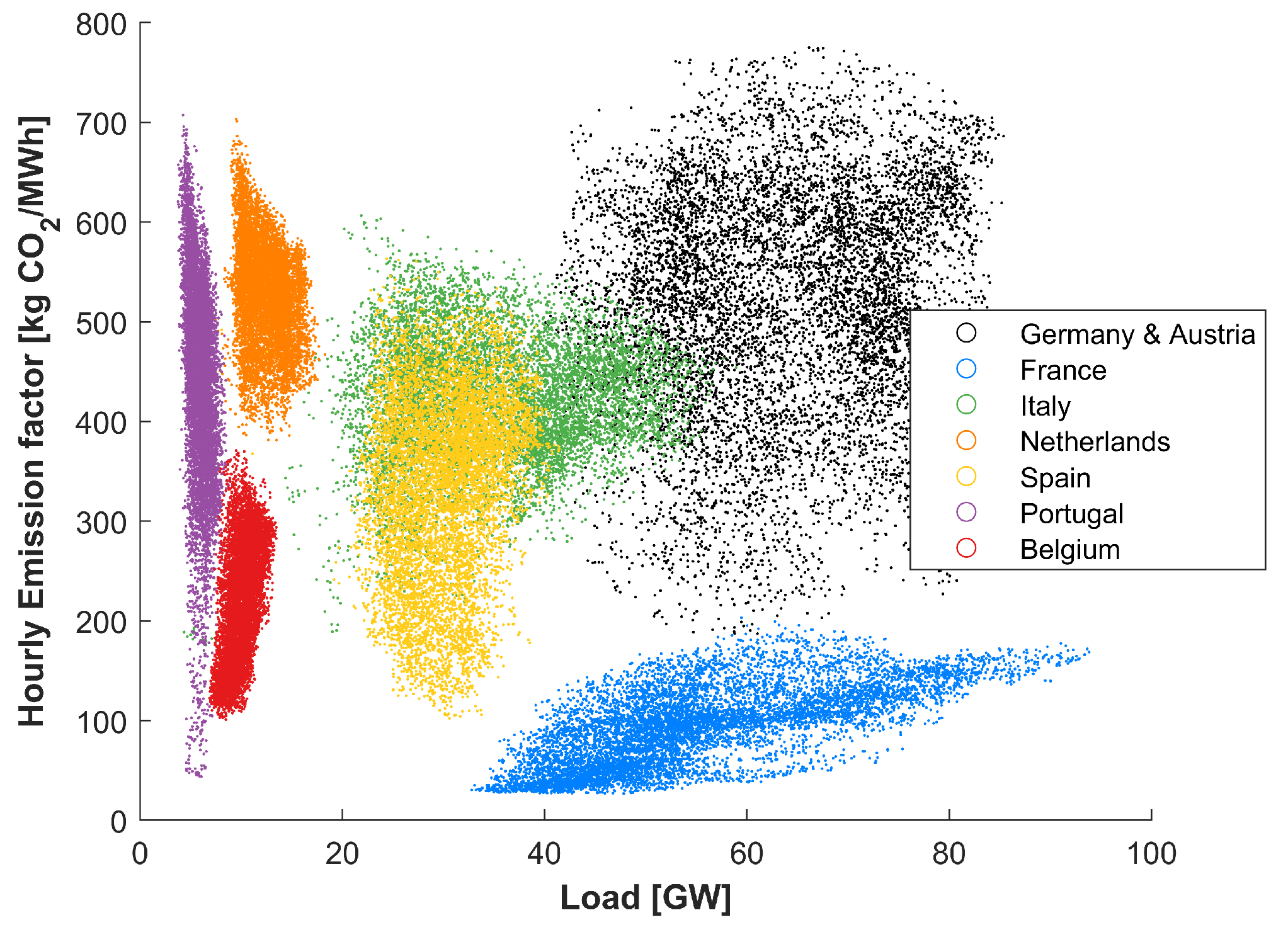
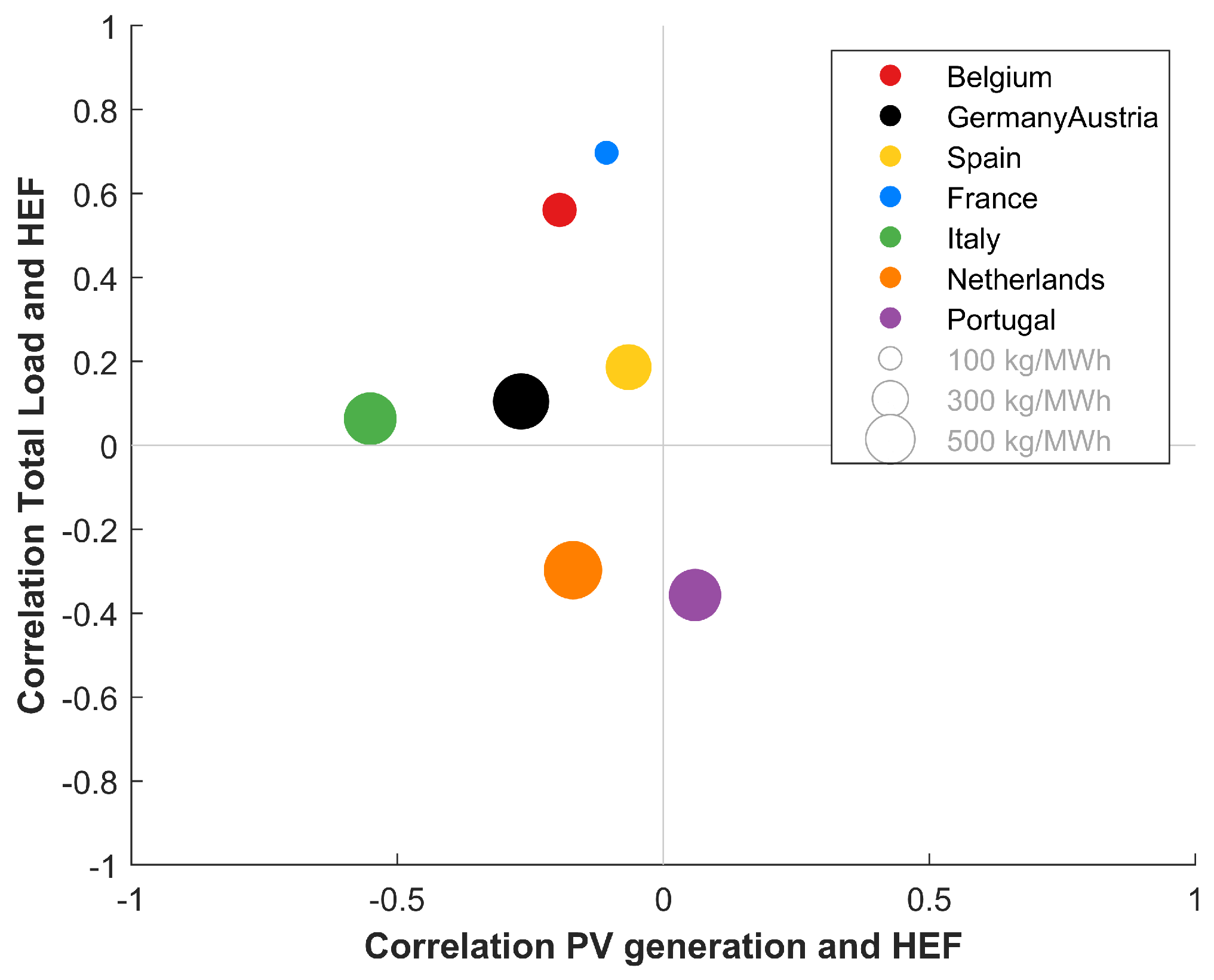
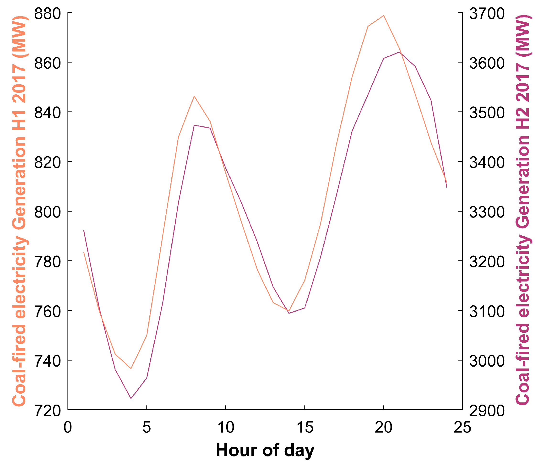
3.1. Hourly Emission Factors

To use time-varying emission factors in the LCA of the prosumer concepts, HEFs for all seven bidding zones were constructed. Note that Austria and Germany were still combined in one bidding zone in 2017, before being separated in late 2018. The time series of the HEFs of the seven bidding zones in 2017 are added to this paper as a Supplementary file.
Figure 2 shows the distribution of all HEFs for the seven bidding zones in 2017. A bidding zone is a geographical area where electricity trading takes place without transport restrictions within their boundaries [1]. From this figure, several observations can be made. The differences between H E F gen and H E F con is caused by the electricity import of a country: when imported electricity has a lower EF than the H E F gen of a country, this results in a lower H E F con of that country. This is seen most in Italy and the Netherlands. Italy imports much electricity from Switzerland and France, which have low EFs. The Netherlands has very high H E F gen , which means import of electricity mostly results in a lower H E F con , but the main difference is caused by the substantial electricity import from Norway which has a low EF. Belgium, on the other hand, has a higher H E F con than H E F gen because it imports a lot of electricity from the Netherlands. This relates to the low HEFs in general for France and Belgium, which is largely due to a high share of nuclear power generation in these countries (72.6% and 49.4%, respectively). Nuclear power generation has the lowest emission factor of all sources; around 12 kg/MWh. The multi-modal shape of these distributions also reflects the general load profile; the first mode reflects night hours where nuclear has an even larger share.
Figure 2 also shows the large variation in H E F con for some bidding zones, especially Spain, Portugal, Germany and Austria. Figure 3 explores this in more detail, showing the H E F con depicted against a country’s total electricity load. Germany and Austria have a large variation both in load and in H E F con . Spain and especially Portugal on the other hand, have a large variation in H E F con , while having relatively low variation in load. This could be explained by having a high share of RES in the generation mix. Also, some countries show an upward trend in H E F con with increasing load, mainly France and Belgium, while others show a negative trend (mainly the Netherlands). This is related to nuclear energy supplying the base load in the former, while coal serves as base load in the latter. The correlations between the load and the H E F con are shown in Figure 4. This figure also shows the correlation between PV-generated electricity and H E F con . A negative correlation can be expected, because in general the EF of PV is lower than the average of the generation mix. This is true for all countries, except for Portugal. A possible explanation is that electricity load serves as a confounding variable; an increased electricity demand in hours with high shares of PV-generated electricity, for example because of air-conditioning, could also lead to more coal-fired electricity generation, ultimately increasing the H E F con . This means that PV systems can have additional GHG emission reduction potential in Portugal, because new systems would replace a relatively dirty electricity mix. In Section 3.2, Section 3.3 and Section 3.4, H E F con is used for the determination of emissions related to electricity and for readability purposes is referred to as HEF (i.e., without subscript “con”).

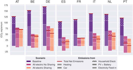
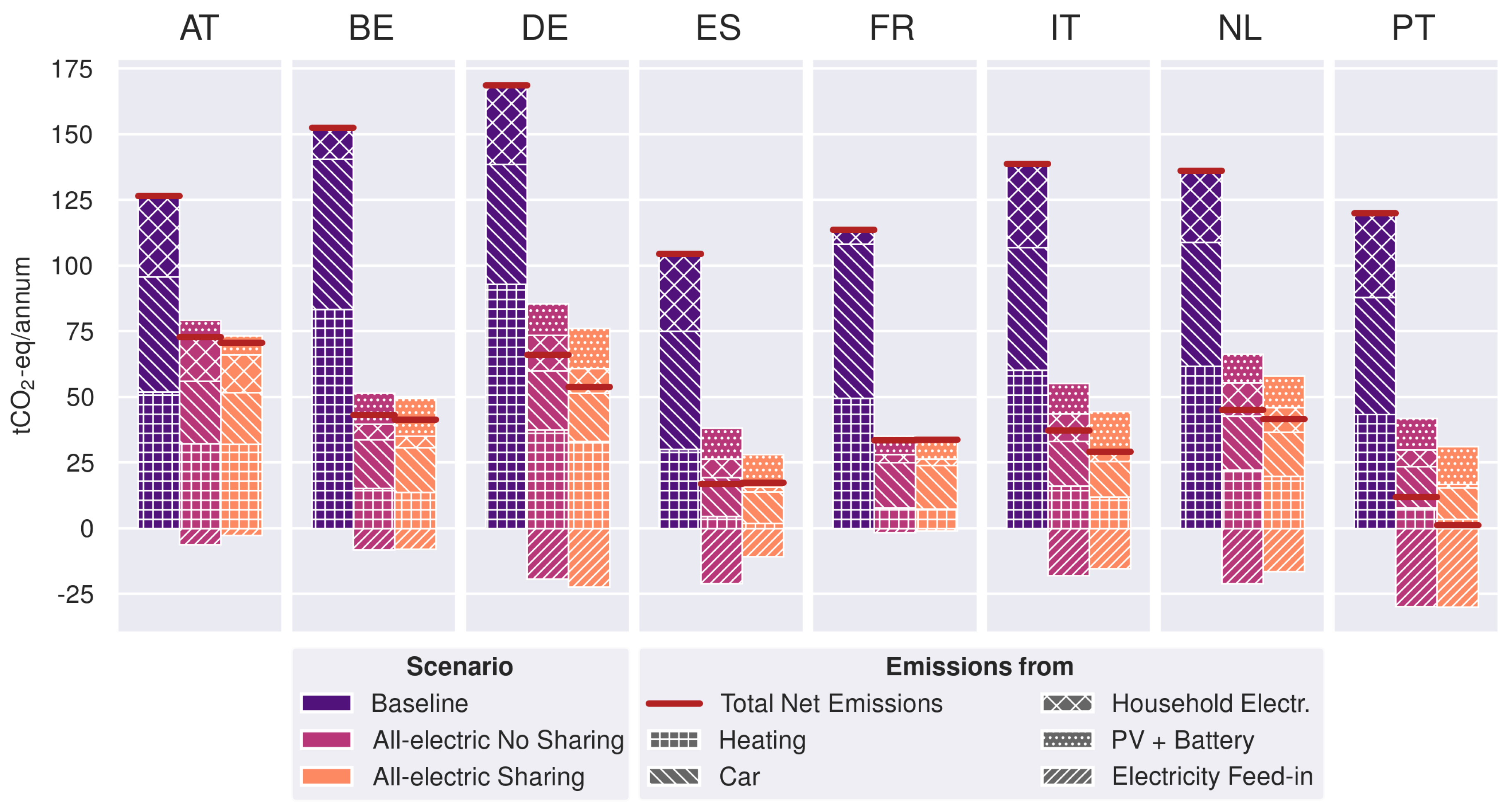
3.2. GHG Emissions of European Communities

In Figure 5 we provide an overview of the total annual community-level GHG emissions among the different technologies and grid-interaction scenarios for all countries. In this figure we see that for most countries the switch towards fully electrified heating and personal transport has a profound effect on total GHG emissions of the communities. This effect is moderated by the HEFs of a country: e.g., in France, the effect is much lower than in the other countries. Furthermore, investments in (mainly) PV can decrease the annual emissions of communities substantially, provided that the economic parameters of installing and operating PV systems are suitable. Also here, we see large differences between the countries. In France, the PV and battery result in more emissions than not having PV and a battery; this can be explained by the higher emission factor of PV compared to nuclear: 84 kg/MWh versus 13 kg/MWh, respectively. Furthermore, PV electricity is generated in hours with a relatively low HEFs (see Figure 4), which results in a lower impact of PV installment. PV and battery can have the most impact in Portugal. This is the result of favourable policies in Portugal combined with high solar irradiation, which leads to a high value of installed PV capacity. Furthermore, the HEFs of Portugal are relatively high, and especially high in hours with much PV-generated electricity. This even leads to the Portuguese Community having negative net emissions. The high GHG emission reduction potential of PV in the Netherlands is also remarkable, as this is the country with the lowest solar irradiation of all investigated countries. Policies in the Netherlands are relatively favourable, but the very high hourly emission factors also play an important role. Energy sharing leads to GHG emissions reduction in all countries: emissions are lower in the All-electric–Sharing scenario than in the All-electric–No Sharing scenario. This can mostly be explained by the higher amount of installed PV capacity as a result of energy sharing (see Table 1). However, the differences are larger in some countries than in other countries; the higher the self-consumption benefits, the larger the impact of energy sharing (through higher installed capacity).

3.2.1. Baseline Scenario

In the baseline scenario, generally speaking, the largest shares of the total community emissions are from heating and using the passenger car. Due to a relatively low heat demand in especially Spain and Portugal, contributions of heating, car and household electricity use in the baseline scenario are roughly equal.
The differences between the countries for the emissions from heating result mainly from the different heating demand in each of the countries, but are also a result of the different technologies used for space heating. Across Europe, the predominant heating technology is based on (condensing) natural gas boilers, but some countries, like Austria, also have large shares of biomass based district heating, with relatively low emission factors. Warm countries like Portugal and Spain have a relatively low heating demand, resulting in low emissions for heating.
For car usage, the difference between the countries are solely the result of the different driving behaviors (km driven per car per year), as we have assumed the same types of cars are used in each country. Car usage contributes a significant share of overall emissions for the baseline scenario.

3.2.2. All-Electric Scenarios

In the all-electric scenarios, we observe a strong reduction in overall community GHG emissions for most countries. Due to the shift from ICEVs to BEVs, and from largely fossil fuel-based heating to fully electric heating, emissions are reduced strongly for most countries.
Austria, having a relatively low emission factor for heating in the baseline scenario, shows a relatively modest reduction in heating emissions, compared to for instance Belgium, where the application of electricity for space heating, combined with the low grid emission factor results in a strong decrease of GHG emissions. In Portugal and Spain, the low heat demand, high PV yield, and application of HPs nearly reduces the emissions from heating to zero in the scenarios with installed PV.
Emissions from car usage also strongly drop in all countries. The application of electricity for personal transport strongly reduces GHG emissions, despite the fact that manufacturing of BEVs is much more GHG intensive compared to manufacturing of ICEVs. Especially in countries with very low grid emission factors (France, Belgium) or in scenarios with high PV generation (Spain, Portugal, Italy), emissions from personal transport are lowered very substantially.

3.2.3. Benefits of Community Energy-Sharing

One of the goals of the PVP4Grid project was to establish the benefits of energy sharing in European communities. Our results indicate that the benefits of energy sharing, in terms of GHG emissions, are affected by a variety of parameters.
In six of the eight countries, energy sharing in the community (further) reduces the GHG emissions compared to the No sharing scenario. In most cases, this is the result of increased deployment of PV. In the energy-sharing communities, more of the generated PV electricity can be used within the community, which reduces grid feed-in, and thus allows for a higher installed PV capacity in countries with financial constraints for grid feed-in. The fact that less electricity is fed into the grid can however also hamper the GHG emission reduction potential in countries with high grid emission factors.

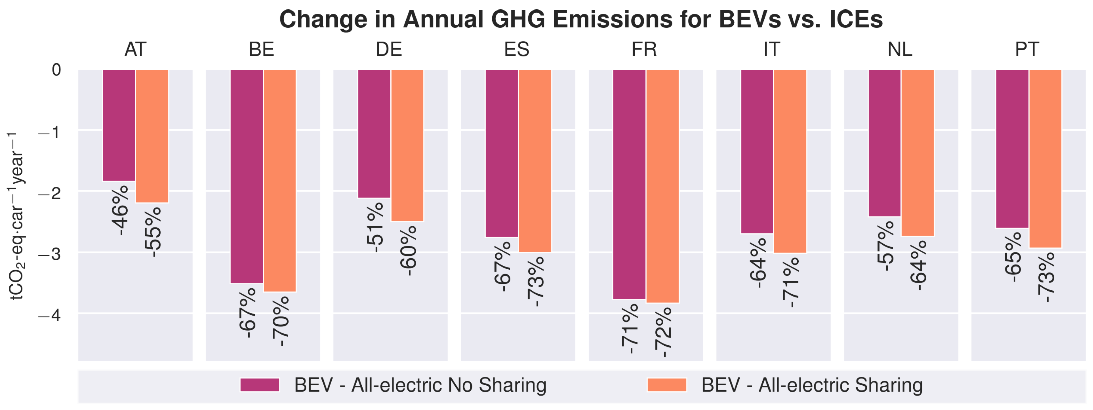
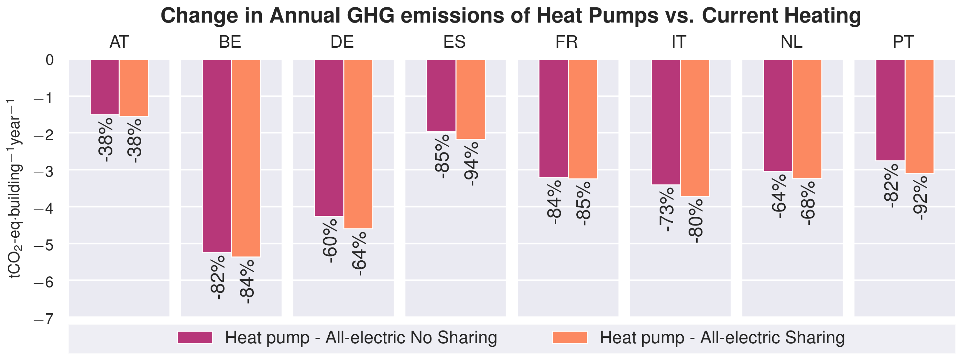
3.3. Normalized GHG Emission Reduction Potentials

To assess the effects of several specific technology transitions, we have analyzed the normalized GHG reductions of BEVs, heat-pumps and PV and BESS. In Figure 6, Figure 7, Figure 8 and Figure 9 we show the reduction in GHG emissions resulting from the transition towards these technologies. To focus on the specific technologies, and avoid the effects from country-level differences of e.g., installed PV capacity resulting from the economic modelling, we normalize the values to a consistent functional unit: 1 BEV for car usage, 1 building for heat supply, 1 kWp for PV systems, and 1 kWh for BESS.

3.3.1. Transition from ICEVs to BEVs

In Figure 6 we see that for all countries, in both scenarios with BEVs, a strong reduction is observed in the GHG emissions resulting from car usage. Emissions from car usage are reduced by 46 to 73%, depending on the source of electricity used for charging, and its associated emission factor.
Absolute reductions in car usage emissions are largest in Belgium and France, where emissions from burning fossil fuels are replace with BEVs charged with very low-emission grid and PV electricity. In Spain and Portugal, due to the high yield of PV systems, a large part of the charging of BEVs is performed with PV electricity, and hence relative reductions are of similar magnitude compared to Belgium and France. Smaller absolute and relative reductions in emissions are observed for the other countries, where the grid emission factor is relatively high and/or PV system yield is substantially lower, hence less charging is performed with PV electricity.

3.3.2. Transition from Fossil Fuel Heat to Heat Pumps

The results for the transition in heat supply from largely fossil fuel-based heat generation to electrified heat generation using HPs is shown in Figure 7. Here, we see a much larger variation between the countries, both in observed absolute and relative changes. Overall, emissions from heat supply drop by 38% to 94%, depending on the GHG intensity of the current heat supply, overall heat demand, and the GHG intensity of the country electricity mix.
In Belgium, the largest absolute reduction of GHG emissions from heat supply is observed. The shift from fossil fuel-based heating to electrified heating with heat-pumps benefits from the low grid emission factor in this country. In France a similar relative reduction is observed, but the absolute reduction is much lower since the heat demand in France is also lower.
In Portugal and Spain, the largest relative reduction in heat supply emissions are found. Due to a combination of low heat demand in these countries, high generation of PV electricity which can be applied in HPs for large parts of the year, emissions are strongly reduced, almost to zero in the Sharing scenario.

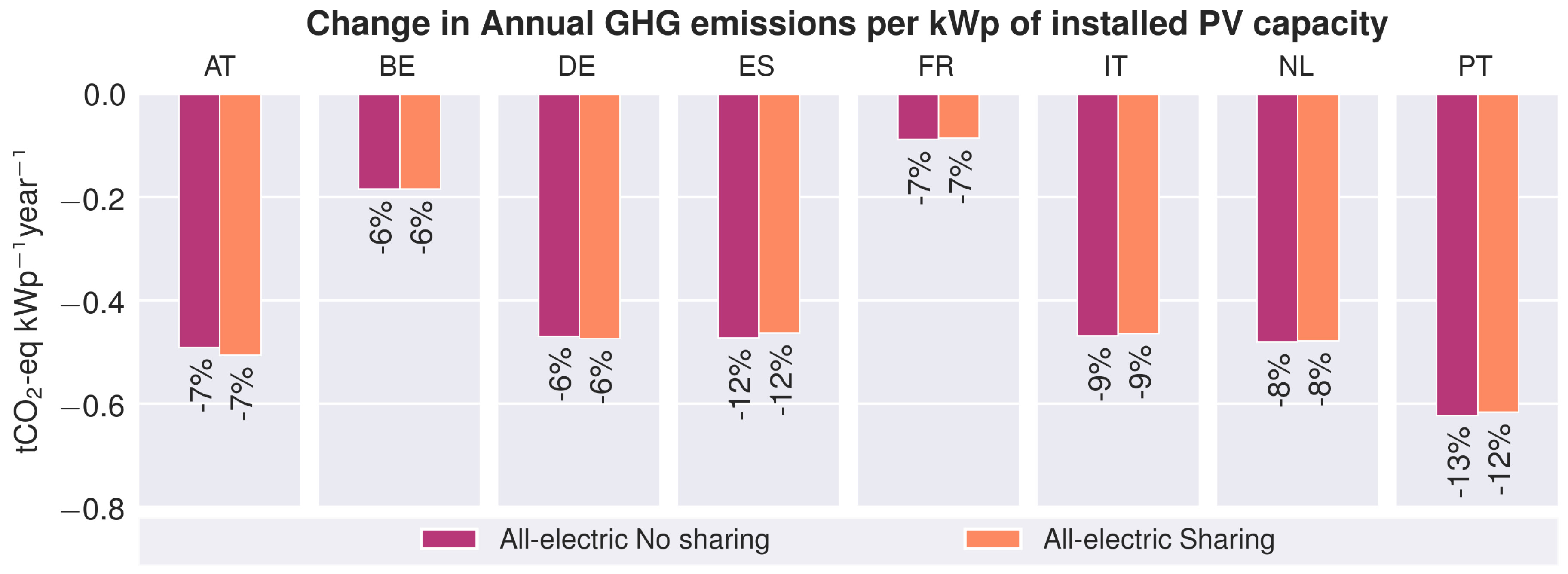
3.3.3. Transition from Grid Consumption to PV Generation

To see and compare the potential for GHG emission reduction of PV systems in the eight countries, we show in Figure 8 the total reductions in GHG emission from electricity supply in the communities in tCO 2 -eq·kWp 1 year 1 . We also present the relative reduction in percent per kWp average per building in the community.
In the all-electric scenarios, the relative reduction of GHG emissions from electricity supply ranges from 6% to 12%, due to the much higher electricity demand in the all-electric scenarios. Absolute reductions are roughly equal for Austria, Germany, Spain, Italy and the Netherlands, and much lower for France and Belgium. In these latter two countries, emissions from electricity consumption are already quite low due to the low grid emission factors in these countries. In Portugal, absolute and relative reductions are the highest, which results from the fact that there is a positive correlation between PV generation and grid emissions factor (as shown in Figure 4). In other words, during the time that PV electricity is generated, grid emission factors are high, and thus the PV electricity that is generated in Portugal mostly replaces electricity from the grid with high emission factors.

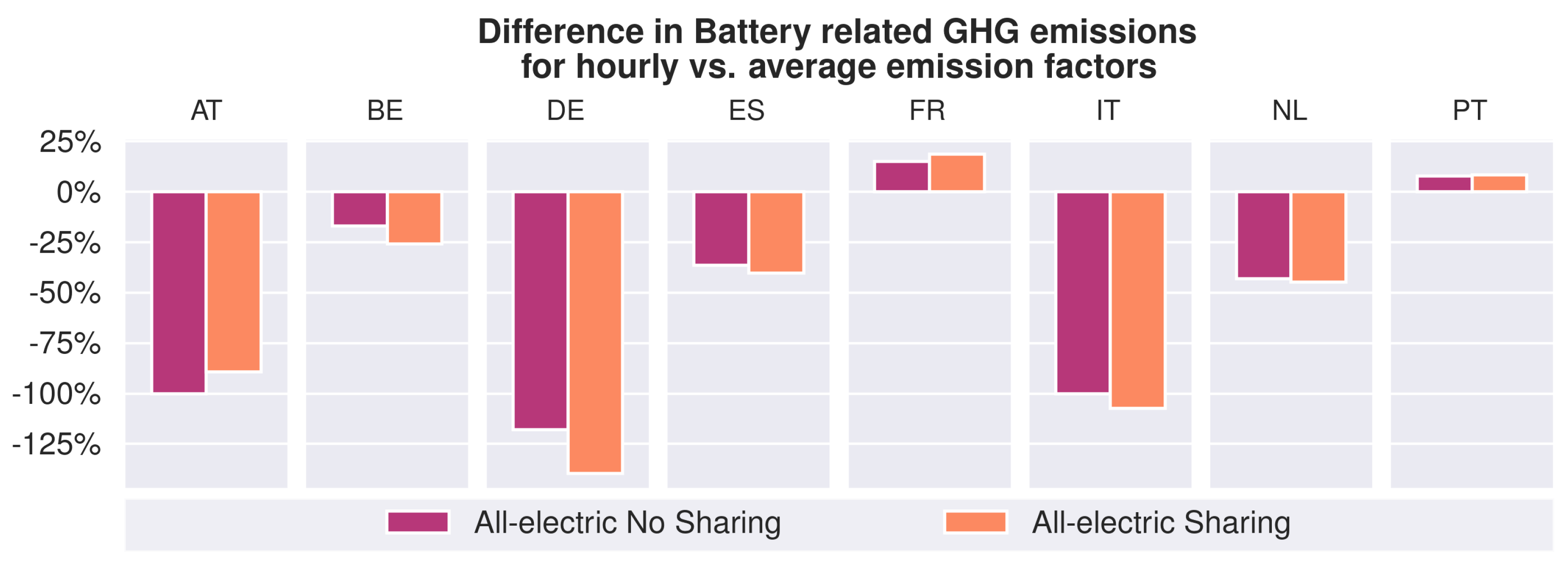
3.3.4. Application of Batteries for Enhanced Self-Consumption of PV Electricity

In the modelling scenarios, relatively small amounts of battery capacities are installed, compared to the installed PV capacities. The batteries are used mainly to store PV electricity that cannot be consumed directly. In theory, batteries could reduce GHG emissions by storing energy at times that grid emission factors are low, and subsequently discharging electricity to the consumers at times that grid emission factors are high. However, since electricity costs for the consumers in the communities do not vary throughout the day in the modelling scenarios from [20], the batteries are used only to store excess PV electricity. In this case, the emissions from battery operation in country j are calculated as follows:
G H G batt , annual , j = t = 1 t = 8760 E charge , t , j · H E F con , t , j t = 1 t = 8760 E discharge , t , j · H E F con , t , j + G H G batt , manufacture
Here, the first summed term represents the emissions attributed to BESS, as PV electricity is prevented from being fed into the grid, which would replace grid electricity and thus create “negative” emissions. The second summed term represents the emissions that are avoided by BESS discharging, replacing the need for grid consumption with the associated HEFs. The final term in Equation (5) represents the emissions resulting from manufacturing of the BESS.
As shown in Figure 9, the installation and operation of batteries results in added GHG emissions in all countries. Emissions are increased when installing batteries, due to the facts that feed-in of PV electricity reduces GHG emissions in our modelling scenario, battery charging/discharging has an efficiency lower than 100%, and the difference between HEFs during daytime and nighttime is relatively small. The largest increase in emissions is observed for Portugal, where the HEFs are higher during the daytime (as discussed before), hence it would be more beneficial to feed-in PV electricity during the day, rather than storing it for use at a later time.

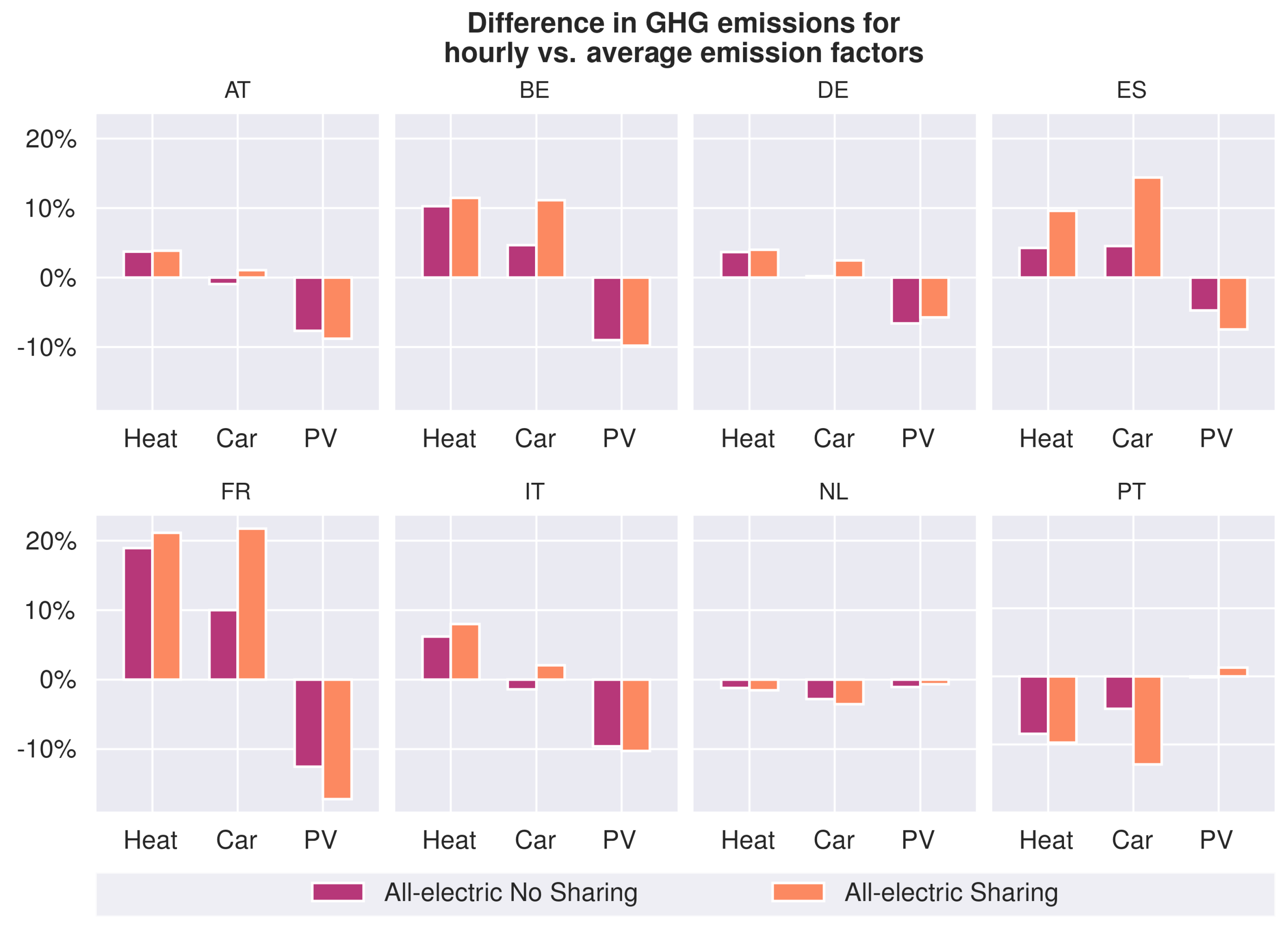
3.4. Difference between AEF and HEF in Determining GHG Emissions

As we discuss in the introduction, the benefits of using HEFs instead of AEFs is that with HEFs the time-based aspect of variable renewable energy generation as well as variable electricity demand is taken into account. Since emission profiles of electricity generation varies throughout the day and over the year, and the all-electric technologies discussed here also do not have constant electricity demand during the day and throughout a year, using HEFs should more accurately account for the effects of these variation on calculated annual GHG emission. In Figure 10 and Figure 11, we compare the application of HEFs vs. AEFs.
In Figure 10, we show the differences between using HEFs and AEFs for our results for car usage, heat supply and PV electricity generation. This figure mainly reflects the different intra-day and seasonal profiles of grid emission factors.
For both heat demand and car usage, we mostly see that the use of HEFs results in higher emissions than when using AEFs. This is especially the case for France and Belgium. For these countries, especially for heat supply, the electricity demand occurs during periods in the year when emission factors are higher than average. As PV systems are added to the communities, the difference between HEFs and AEFs becomes larger, as a relatively larger share of heat demand related electricity from the grid is used during winter. Since car usage is constant throughout the year the difference between HEFs and AEFs for the baseline scenario is much smaller, but grows more strongly as PV systems are added. Contrasting to the results for most countries, are the results for Portugal. Here, grid emission factors are somewhat lower during winter, and during times of limited or no PV generation.
In most countries, the difference between HEFs and AEFs is negative for emission reductions of PV systems. This means that when using HEFs, the emission reductions calculated for PV systems are smaller compared to when using AEFs. This is the result of the fact that in most countries, emission factors are generally lower during the day (and in summer). Only in Portugal, where grid emission are in fact higher during the times of PV generation, this result is not observed. In Figure 11, we present the comparison of using HEFs vs. AEFs for BESS. In this figure, we only show the emissions related to charging and discharging of the BESS, without manufacturing emissions, to highlight the effects of HEFs vs. AEFs (otherwise the emission were calculated according to Equation (5)).
The results show that the emissions attributed to battery charging and discharging are generally lower when using HEFs compared to AEFS, except for Portugal and France. Using HEFs, the emissions in the other countries are lower, as batteries are charged during the day, when grid emission factors are low, and discharged during the night, when grid emission factors are higher. For Austria, Germany and Italy, the difference between HEFs and AEFs is especially large, due to the clear difference of HEFs between charging (daytime) and discharging (nighttime).

4. Conclusions and Discussion

In this research, the GHG emission reduction potential of EVs, HPs, PV and BESS was determined in eight countries: Austria, Belgium, France, Germany, Italy, the Netherlands, Portugal and Spain. Hereby, HEFs were being used to determine the emissions related to electricity use. The selection of technologies and countries represents the important role of electrification in the built environment in transitioning to a sustainable future, taking into account different climatic regions in Europe. Results show there are large differences between countries regarding there HEFs, with France and Belgium being on the lower end of the spectrum (because of high shares of nuclear power plants in their generation mix) Austria, Germany and the Netherlands on the higher end of the spectrum (high shares of coal-fired power plants) and the southern countries Italy, Portugal and Spain in the middle of the spectrum (high shares of renewables, medium shares coal-fired power plants). These results have a strong moderating effect on the GHG emission reduction potential of the technologies. Most technologies have substantial GHG emission reduction potential in all countries. BESS are the exception, as these increase emissions in all countries because of losses in the conversion of electricity. These results imply that from a European GHG emission reduction perspective, it is important to not only focus on e.g., installing PV in countries with high values of solar irradiation, but also look at the current electricity mix of the countries. Furthermore, we have seen that energy sharing leads to an increased GHG emission reduction potential, because energy sharing leads to higher PV capacities—this can be an important notion in designing policies stimilating the deployment of renewable energy. Lastly, we have demonstrated the importance the timing of consuming electricity, signifying the added value of HEFs over AEFs. This is an important finding both from a practical as a scientific perspective, as the AEF is more commonly used in GHG impact assessments.
These findings may be somewhat limited by the data accuracy. As our study entails an extensive amount of data, large databases were used to generate the results (i.e., the transparency data set of ENTSO-E [58] and the ecoinvent database [54]). In some cases, these databases can have missing data (as shown in Appendix A) or are not up-to-date for individual data points (as in the case of e.g., the PV emission factor). Furthermore, the GHG emission reduction potentials of the European Communities are necessarily impacted by the specific configuration of the community, hence, it is important to interpret these results along with the normalized GHG emission reduction potentials that we also reported.
Future research could increase both the geographical and time scope. It should be taken into account that our study focused on one year, namely 2017. With changing generation mixes, the GHG emissions of the technologies almost certainly will change in the future due to electricity consumption or feed-in. Changes in generation mixes can be included in future research in order to make a full LCA. As we have found large differences in HEFs between countries, the analysis can be extended to include even more countries, e.g., other regions within Europe, or countries on different continents. Furthermore, we have shown that fluctuation of HEFs impact the GHG emissions of a technology. Some technologies, mostly BESS and BEVs, have the potential to shift demand over time. The generated HEF profiles can be used as data input for optimization frameworks. This could further increase their GHG emission reduction potential, or in case of BESS reverse the adverse impact. Future research could attempt to quantify this additional potential, and in similar fashion of our study, determine in which countries flexible assets can have the most climate mitigation impact. In this context, the use of marginal emission factors (i.e., the emissions of the power plant that operates at the margin, reflecting the change in emissions as result of a change electricity demand or supply [59] should also be considered.

Supplementary Materials

The hourly emission factor profiles of Belgium, Spain, France, Italy, The Netherlands, Portugal, Germany and Austria for 2017 are available at: https://www.mdpi.com/1996-1073/12/23/4440/s1.

Author Contributions

Conceptualization, W.S. and A.L.; methodology, W.S. and A.L.; validation, W.S. and A.L.; formal analysis, W.S. and A.L.; investigation, W.S. and A.L.; resources, W.S., and A.L.; data curation, W.S. and A.L.; writing–original draft preparation, W.S. and A.L.; writing–review and editing, I.L., W.v.S., W.S. and A.L.; visualization, W.S. and A.L.; supervision, I.L. and W.v.S.; funding acquisition, W.v.S.

Funding

This research was funded by the European Union’s Horizon 2020 research and innovation program under grant agreement No 764786 (project PV-Prosumers4Grid).

Acknowledgments

The authors would like to thank Johannes Radl and Andreas Fleischhacker (TUW) for their modelling work on which this study is based, as well as their help in giving insight in these modelling results.

Conflicts of Interest

The authors declare no conflict of interest. The funders had no role in the design of the study; in the collection, analyses, or interpretation of data; in the writing of the manuscript, or in the decision to publish the results.

Abbreviations

The following abbreviations are used in this manuscript:
Nomenclature
AEFAverage Emission Factor
BESSBattery Energy Storage Systems
BEVBattery Electric Vehicle
DSMDemand Side Management
EFEmission Factor
GHGGreenhouse Gas
HEFHourly Emission Factor
HPHeat Pump
ICEVInternal Combustion Engine Vehicle
LCALife-Cycle Assessment
LCILife-Cycle Inventory
PHEVPlugin Hybrid Electric Vehicle
PVPhotovoltaics
RESRenewable Energy Sources
TSOTransmission System Operator
Indices
jCountry
kGenerator type
lCountry imported from
tHour
Variables
E G 2 L Electricity flow from grid to consumer
E PV feed in Electricity flow from PV system to grid
E F car Emission factor for car transport in gCO 2 -eq passenger 1 · km 1
E F heat Emission factor for heat supply in gCO 2 -eq MJ thermal 1
G H G cons Green House Gas emissions of electricity consumption
G H G gen Green House Gas emissions of electricity generation
G H G HV Green House Gas emissions of electricity on high-voltage lines
H E F cons Hourly Emission Factor of electricity consumption
H E F gen Hourly Emission Factor of electricity generation
H E F HV Hourly Emission Factor of electricity on high-voltage lines

Appendix A. Explanation for Treatment of Missing Data

Appendix A.1. Explanation for Treatment of “Other” Categories

ENTSO-E reports two other generation categories: “Other–Actual Aggregated” and “Other Renewable”. The share of these categories in the total electricity generation is reported in Table A1. Furthermore, to validate the generation data, a check was performed with the power statistics reported in (ENTSO-E, 2019c). Table A1 also shows the correlation between the generation (minus the net export) and this total load. What stands out in Table A1 is the high share of Other for Italy (31.5%), and the low correlation with the power statistics for the Netherlands (0.548). Therefore, data of two countries received more attention, which is elaborated on later. For the other six countries, the Other categories are proportionally attributed to the known generation data. So Other Renewable is proportionally attributed to the generation of renewable sources (biomass, hydro, solar, geothermal and wind) in the relevant hour. Other—Actual Aggregated is proportionally attributed to non-renewable generation for that hour.
Table A1. Shares of other categories and correlation transparency and power statistics ENTSO-E [55,58].
CountryOther (% of Total Generation)Other Renewable (% of Total Generation)Correlation with ENTSO-E Power Stats
Belgium6.2N.A.0.950
FranceN.A.N.A.0.988
Germany and Austria6.80.30.981
Italy31.50.00.973
NetherlandsN.A.N.A.0.548
Portugal0.6N.A.0.941
Spain0.20.30.950

Appendix A.2. Explanation for Allocation of Missing Data in Italy

Attributing the Other generation proportionally to the known generation values could lead to incorrect results, for example if one generation source has better data availability than the other. Therefore, data report by the Italian TSO Terna was directly investigated, to be able to validate the generation data per source.

Appendix A.2.1. Biomass

Terna reports the hourly electricity generated from biomass [60]. These values are substantially higher than the values obtained from data transparency: average of 344 MW over 2017 on transparency, while the data reported by Terna have an average of 1943 MW. This explains 17% of the Other category.

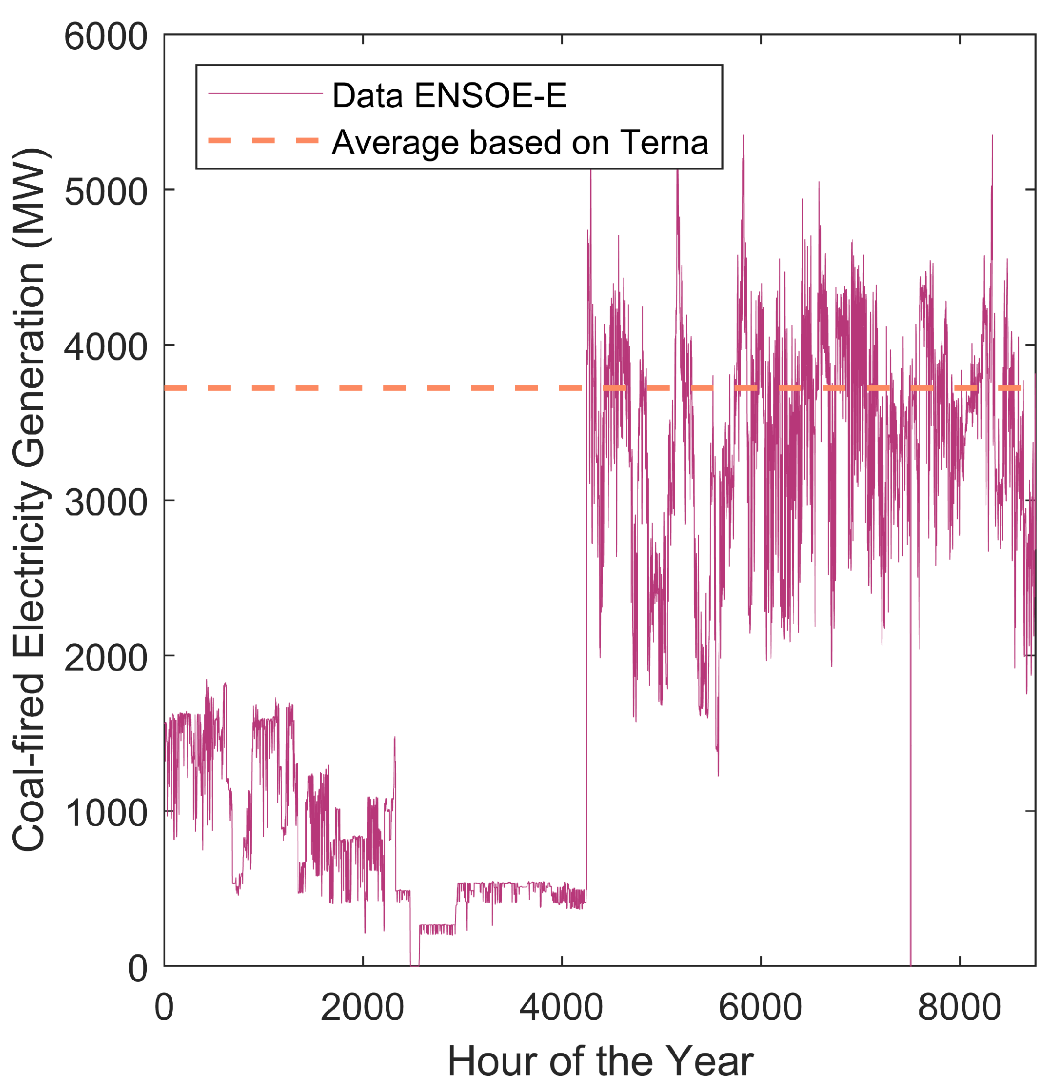
Appendix A.2.2. Coal

As can be seen in Figure A1, the coal-fired electricity generation in the second half of 2017 as reported in (ENTSO-E, 2019a) is in line with the yearly average from 2017 as reported by Terna (Terna, 2019). On 26 June, the coal-fired electricity generation increases from 495 MW from 22:00–23:00 to 3968 MW from 23:00 to 24:00.
It can be concluded that data are missing for the first half of 2017. There are two options to scale up the coal generation for the first half of 2017:
  • Assume coal provides baseload power, take a fixed load factor and calibrate the load factor to be in line with the total of coal as reported by Terna.
  • Multiply the available data by a factor which is calibrated to be in line with the total of coal as reported by Terna.
To decide this, we analyzed if coal could be seen as purely baseload fuel; Figure A2 provides insight on this. As can be seen, the first half and the second half show a similar pattern, with slightly higher generation in a few hours in the morning and the evening. As the data from the second half of 2017 can be considered reliable, we conclude that coal does not serve solely as baseload. Therefore, we decided to increase the coal load by a flat factor for the first half of 2017. For the period with missing data, we see two distinct periods: until 7 April 23:00, the average coal-fired electricity generation was 1104 MW, from 7 April 23:00 to 26 June 23:00 423 MW. For both periods, the data are scaled to be in line with the Italian average.
Figure A1. Reported coal generation in Italy in 2017 in [55] and the average coal-based electricity generation reported by [60].
Energies 12 04440 g0a1
Figure A2. Average hourly coal-fired electricity generation in Italy in first half 2017 (left y-axis) and second half 2017 (right y-axis).
Energies 12 04440 g0a2

Appendix A.2.3. Fossil Oil and Fossil Gas

For fossil oil and fossil gas, no long periods of missing data were found. Therefore, it was concluded that these only part of generation from these sources was reported. The totals taken from the transparency data base were 71.7 TWh for gas and 1.34 TWh for oil. Terna reported totals of 140 TWh and 4.1 TWh, respectively. Therefore, we multiplied the generation values from transparency data by 1.96 for gas and 3.13 for oil.

Appendix A.3. Explanation Missing Data The Netherlands

For the Netherlands, we assumed that coal would run as baseload, based on [48]. Two of the six coal-fired power plants were closed on 1 July 2017. We set the electricity generation from coal as a fixed percentage of the capacity in that hour (i.e., the load factor over 2017). This load factor was determined using the total electricity generated from coal that was reported by the Dutch statistics agency CBS [61]. The remaining gap between generation values in transparency data, and total load reported in power statistics, was attributed to gas-fired power plants. The new total is 9.6% higher than the statistics reported by CBS. In [62], according to the Dutch TSO, TenneT, it is stated that the data should be corrected after official statistics are reported by CBS. We followed this notion, and corrected the total gas-fired electricity generation to be in line with the official statistics.

References

  1. European Commission. Regulation of the European Parliament and of the Council on the Internal Market for Electricity; European Union: Brussels, Belgium, 2016. [Google Scholar]
  2. European Commission. Electrification of the Transport System: Studies and Reports; Technical Report; European Union: Brussels, Belgium, 2017; Available online: http://ec.europa.eu/newsroom/horizon2020/document.cfm?doc_id=46372 (accessed on 6 November 2019).
  3. IEA. Perspectives for the Clean Energy Transition; Technical Report; IEA: Paris, France, 2019. [Google Scholar]
  4. IEA. World Energy Outlook 2018; Technical Report; IEA: Paris, France, 2018. [Google Scholar]
  5. Schmela, M.; Beauvais, A.; Chevillard, N.; Paredes, M.G.; Heisz, M.; Rossi, R.; China Photovoltaic Industry Association (CPIA); Whitten, D.; US Solar Energy Industries Association. Global Market Outlook: 2019–2023; Technical Report; SolarPower Europe: Brussels, Belgium, 2019. [Google Scholar]
  6. Kubli, M.; Loock, M.; Wüstenhagen, R. The flexible prosumer: Measuring the willingness to co-create distributed flexibility. Energy Policy 2018, 114, 540–548. [Google Scholar] [CrossRef]
  7. Fischer, D.; Madani, H. On heat pumps in smart grids: A review. Renew. Sustain. Energy Rev. 2017, 70, 342–357. [Google Scholar] [CrossRef]
  8. Litjens, G.; Worrell, E.; van Sark, W. Lowering greenhouse gas emissions in the built environment by combining ground source heat pumps, photovoltaics and battery storage. Energy Build. 2018, 180, 51–71. [Google Scholar] [CrossRef]
  9. Staffell, I.; Pfenninger, S. The increasing impact of weather on electricity supply and demand. Energy 2018, 145, 65–78. [Google Scholar] [CrossRef]
  10. Eggimann, S.; Hall, J.W.; Eyre, N. A high-resolution spatio-temporal energy demand simulation to explore the potential of heating demand side management with large-scale heat pump diffusion. Appl. Energy 2019, 236, 997–1010. [Google Scholar] [CrossRef]
  11. Mwasilu, F.; Justo, J.J.; Kim, E.K.; Do, T.D.; Jung, J.W. Electric vehicles and smart grid interaction: A review on vehicle to grid and renewable energy sources integration. Renew. Sustain. Energy Rev. 2014, 34, 501–516. [Google Scholar] [CrossRef]
  12. Sundström, O.; Binding, C. Flexible charging optimization for electric vehicles considering distribution grid constraints. IEEE Trans. Smart Grid 2012, 3, 26–37. [Google Scholar] [CrossRef]
  13. Yong, J.Y.; Ramachandaramurthy, V.K.; Tan, K.M.; Mithulananthan, N. A review on the state-of-the-art technologies of electric vehicle, its impacts and prospects. Renew. Sustain. Energy Rev. 2015, 49, 365–385. [Google Scholar] [CrossRef]
  14. Schram, W.L.; Lampropoulos, I.; van Sark, W.G.J.H.M. Photovoltaic systems coupled with batteries that are optimally sized for household self-consumption: Assessment of peak shaving potential. Appl. Energy 2018, 223, 69–81. [Google Scholar] [CrossRef]
  15. Katsanevakis, M.; Stewart, R.A.; Lu, J. Aggregated applications and benefits of energy storage systems with application-specific control methods: A review. Renew. Sustain. Energy Rev. 2017, 75, 719–741. [Google Scholar] [CrossRef]
  16. Lampropoulos, I.; Alskaif, T.; Blom, J.; van Sark, W. A framework for the provision of flexibility services at the transmission and distribution levels through aggregator companies. Sustain. Energy Grids Netw. 2019, 17, 100187. [Google Scholar] [CrossRef]
  17. Siano, P. Demand response and smart grids—A survey. Renew. Sustain. Energy Rev. 2014, 30, 461–478. [Google Scholar] [CrossRef]
  18. Dóci, G.; Vasileiadou, E. “Let’s do it ourselves” Individual motivations for investing in renewables at community level. Renew. Sustain. Energy Rev. 2015, 49, 41–50. [Google Scholar] [CrossRef]
  19. PVP4Grid. PV-Prosumers4Grid—Enabling Consumers to Become PV Prosumers in a System-Friendly Manner. 2019. Available online: https://www.pvp4grid.eu/ (accessed on 1 October 2019).
  20. Fleischhacker, A.; Radl, J.; Revheim, F.; Lettner, G.; Schwabeneder, D.; Auer, H. Quantitative Analyses of Improved PVP4Grid Concepts and Report on Testing; Technical Report; Deliverable D3.2 of the Project PVP4Grid; Technische Universitaet Wien: Vienna, Austria, 2019; Available online: http://www.pvp4grid.eu (accessed on 1 October 2019).
  21. Steg, L.; Vlek, C. Encouraging pro-environmental behaviour: An integrative review and research agenda. J. Environ. Psychol. 2009, 29, 309–317. [Google Scholar] [CrossRef]
  22. Lyons, L. Digitalisation: Opportunities for Heating and Cooling; Publications Office of the European Union: Luxembourg, 2019. [Google Scholar] [CrossRef]
  23. Lindmayer, J.; Anderson, J.; Clifford, A.; Lafky, W.; Scheinine, A.; Wihl, M.; Wrigley, C. Solar Breeder: Energy Payback Time for Silicon Photovoltaic Systems. Report No. SX/111/1Q; Technical Report; Solarex Corporation: Rockville, MD, USA, 1977. [Google Scholar]
  24. Wihl, M.; Scheinine, A. Analysis and simulation of the energy source of the future—The solar breeder. In Proceedings of the 13th Photovoltaics Specialists Conference, Washington, DC, USA, 5–8 June 1978; pp. 908–910. [Google Scholar]
  25. Bhandari, K.P.; Collier, J.M.; Ellingson, R.J.; Apul, D.S. Energy payback time (EPBT) and energy return on energy invested (EROI) of solar photovoltaic systems: A systematic review and meta-analysis. Renew. Sustain. Energy Rev. 2015, 47, 133–141. [Google Scholar] [CrossRef]
  26. Asdrubali, F.; Baldinelli, G.; D’Alessandro, F.; Scrucca, F. Life cycle assessment of electricity production from renewable energies: Review and results harmonization. Renew. Sustain. Energy Rev. 2015. [Google Scholar] [CrossRef]
  27. Pehl, M.; Arvesen, A.; Humpenöder, F.; Popp, A.; Hertwich, E.G.; Luderer, G. Understanding future emissions from low-carbon power systems by integration of life-cycle assessment and integrated energy modelling. Nat. Energy 2017. [Google Scholar] [CrossRef]
  28. Abdul-Manan, A.F. Uncertainty and differences in GHG emissions between electric and conventional gasoline vehicles with implications for transport policy making. Energy Policy 2015. [Google Scholar] [CrossRef]
  29. Bauer, C.; Hofer, J.; Althaus, H.J.; Del Duce, A.; Simons, A. The environmental performance of current and future passenger vehicles: Life Cycle Assessment based on a novel scenario analysis framework. Appl. Energy 2015. [Google Scholar] [CrossRef]
  30. Cerdas, F.; Egede, P.; Herrmann, C. LCA of Electromobility. In Life Cycle Assessment; Springer International Publishing: Cham, Switzerland, 2018; pp. 669–693. [Google Scholar] [CrossRef]
  31. Höltl, A.; Macharis, C.; De Brucker, K. Pathways to Decarbonise the European Car Fleet: A Scenario Analysis Using the Backcasting Approach. Energies 2017, 11, 20. [Google Scholar] [CrossRef]
  32. Kawamoto, R.; Mochizuki, H.; Moriguchi, Y.; Nakano, T.; Motohashi, M.; Sakai, Y.; Inaba, A. Estimation of CO2 Emissions of Internal Combustion Engine Vehicle and Battery Electric Vehicle Using LCA. Sustainability 2019, 11, 2690. [Google Scholar] [CrossRef]
  33. Moro, A.; Lonza, L. Electricity carbon intensity in European Member States: Impacts on GHG emissions of electric vehicles. Transp. Res. Part D Transp. Environ. 2018. [Google Scholar] [CrossRef] [PubMed]
  34. Onat, N.C.; Noori, M.; Kucukvar, M.; Zhao, Y.; Tatari, O.; Chester, M. Exploring the suitability of electric vehicles in the United States. Energy 2017, 121, 631–642. [Google Scholar] [CrossRef]
  35. Wu, Z.; Wang, M.; Zheng, J.; Sun, X.; Zhao, M.; Wang, X. Life cycle greenhouse gas emission reduction potential of battery electric vehicle. J. Clean. Prod. 2018. [Google Scholar] [CrossRef]
  36. Abusoglu, A.; Sedeeq, M.S. Comparative exergoenvironmental analysis and assessment of various residential heating systems. Energy Build. 2013, 62, 268–277. [Google Scholar] [CrossRef]
  37. Blom, I.; Itard, L.; Meijer, A. LCA-based environmental assessment of the use and maintenance of heating and ventilation systems in Dutch dwellings. Build. Environ. 2010, 45, 2362–2372. [Google Scholar] [CrossRef]
  38. Genkinger, A.; Dott, R.; Afjei, T. Combining Heat Pumps with Solar Energy for Domestic Hot Water Production. Energy Procedia 2012, 30, 101–105. [Google Scholar] [CrossRef]
  39. Greening, B.; Azapagic, A. Domestic heat pumps: Life cycle environmental impacts and potential implications for the UK. Energy 2012, 39, 205–217. [Google Scholar] [CrossRef]
  40. Koroneos, C.J.; Nanaki, E.A. Environmental impact assessment of a ground source heat pump system in Greece. Geothermics 2017, 65, 1–9. [Google Scholar] [CrossRef]
  41. Nitkiewicz, A.; Sekret, R. Comparison of LCA results of low temperature heat plant using electric heat pump, absorption heat pump and gas-fired boiler. Energy Convers. Manag. 2014, 87, 647–652. [Google Scholar] [CrossRef]
  42. Ozdogan Dolcek, A.; Tinjum, J.M. Life-cycle assessment of various types of residential ground-coupled heat pump systems: Wisconsin, US case. Sol. Energy 2019. [Google Scholar] [CrossRef]
  43. Shah, V.P.; Debella, D.C.; Ries, R.J. Life cycle assessment of residential heating and cooling systems in four regions in the United States. Energy Build. 2008, 40, 503–513. [Google Scholar] [CrossRef]
  44. Pellow, M.A.; Ambrose, H.; Mulvaney, D.; Betita, R.; Shaw, S. Research gaps in environmental life cycle assessments of lithium ion batteries for grid-scale stationary energy storage systems: End-of-life options and other issues. Sustain. Mater. Technol. 2019, e00120. [Google Scholar] [CrossRef]
  45. Lausselet, C.; Borgnes, V.; Brattebø, H. LCA modelling for Zero Emission Neighbourhoods in early stage planning. Build. Environ. 2019, 149, 379–389. [Google Scholar] [CrossRef]
  46. Lund, K.M.; Lausselet, C.; Brattebø, H. LCA of the Zero Emission Neighbourhood Ydalir. IOP Conf. Ser. Earth Environ. Sci. 2019, 352. [Google Scholar] [CrossRef]
  47. Smith, C.; Burrows, J.; Scheier, E.; Young, A.; Smith, J.; Young, T.; Gheewala, S.H. Comparative Life Cycle Assessment of a Thai Island’s diesel/PV/wind hybrid microgrid. Renew. Energy 2015, 80, 85–100. [Google Scholar] [CrossRef]
  48. Schram, W.; Lampropoulos, I.; Alskaif, T.; Sark, W.V. On the Use of Average versus Marginal Emission Factors. In Proceedings of the 8th International Conference on Smart Cities and Green ICT Systems (SMARTGREENS 2019), Heraklion, Crete, Greece, 3–5 May 2019; SciTePress: Heraklion, Crete, Greece, 2019; pp. 187–193. [Google Scholar]
  49. Ryan, N.A.; Lin, Y.; Mitchell-Ward, N.; Mathieu, J.L.; Johnson, J.X. Use-Phase Drives Lithium-Ion Battery Life Cycle Environmental Impacts When Used for Frequency Regulation. Environ. Sci. Technol. 2018, 52, 10163–10174. [Google Scholar] [CrossRef]
  50. Fares, R.L.; Webber, M.E. The impacts of storing solar energy in the home to reduce reliance on the utility. Nat. Energy 2017, 2, 17001. [Google Scholar] [CrossRef]
  51. Bettle, R.; Pout, C.H.; Hitchin, E.R. Interactions between electricity-saving measures and carbon emissions from power generation in England and Wales. Energy Policy 2006, 34, 3434–3446. [Google Scholar] [CrossRef]
  52. Marnay, C.; Fisher, D.; Murtishaw, S.; Phadke, A.; Price, L.; Sathaye, J. Estimating Carbon Dioxide Emissions Factors for the California Electric Power Sector; Technical Report; Lawrence Berkeley National Laboratory: Berkeley, CA, USA, 2002.
  53. Thomson, R.C.; Harrison, G.P.; Chick, J.P. Marginal greenhouse gas emissions displacement of wind power in Great Britain. Energy Policy 2017, 101, 201–210. [Google Scholar] [CrossRef]
  54. Wernet, G.; Bauer, C.; Steubing, B.; Reinhard, J.; Moreno-Ruiz, E.; Weidema, B. The ecoinvent database version 3 (part I): Overview and methodology. Int. J. Life Cycle Assess. 2016, 21, 1218–1230. [Google Scholar] [CrossRef]
  55. ENTSO-E. Actual Generation per Production Type. 2019. Available online: https://transparency.entsoe.eu/generation/r2/actualGenerationPerProductionType/show (accessed on 10 July 2019).
  56. Eurostat. Passenger Cars, by Type of Motor Energy. 2019. Available online: https://ec.europa.eu/eurostat/data/database (accessed on 1 September 2019).
  57. Fleiter, T.; Elsland, R.; Rehfeldt, M.; Steinbach, J.; Reiter, U.; Catenazzi, G.; Jakob, M.; Rutten, C.; Harmsen, R.; Dittmann, F.; et al. Profile of Heating and Cooling Demand in 2015. Technical Report; Deliverable D3.1 of the Project Heat Roadmap Europe. 2017. Available online: https://heatroadmap.eu (accessed on 1 September 2019).
  58. ENTSO-E. Monthly Hourly Load Values. 2019. Available online: https://www.entsoe.eu/data/power-stats/hourly_load/ (accessed on 10 July 2019).
  59. Harmsen, R.; Graus, W. How much CO2 emissions do we reduce by saving electricity? A focus on methods. Energy Policy 2013, 60, 803–812. [Google Scholar] [CrossRef]
  60. Terna. The Evolution of the Electricity Market: All Da. 2019. Available online: https://www.terna.it/en/electric-system/statistical-data-forecast/evolution-electricity-market (accessed on 10 July 2019).
  61. CBS. Elektriciteit en Warmte Productie en inzet naar Energiedrager. 2019. Available online: https://opendata.cbs.nl/statline/CBS/nl/dataset/80030NED (accessed on 10 July 2019).
  62. ENTSO-E. Specific National Considerations; Technical Report; ENTSO-E, Brussels, Belgium: 2016. Available online: https://docstore.entsoe.eu/Documents/Publications/Statistics/Specific_national_considerations.pdf (accessed on 10 July 2019).
Figure 1. Overview of the ‘typical EU community’ analyzed here. Source: Image adapted from [20].
Energies 12 04440 g001
Figure 2. Violin plot of distribution Generation and Consumption Hourly Emission Factors per bidding zone. Solid line indicates mean, dashed lines the 25% and 75% percentiles. Country codes: BE = Belgium, DE = Germany, AT = Austria, ES = Spain, FR = France, IT = Italy, NL = Netherlands, PT = Portugal.
Energies 12 04440 g002
Figure 3. Country electricity load depicted against its H E F con .
Energies 12 04440 g003
Figure 4. The y-axis depicts the correlation between a Country’s electricity load and its H E F con , the x-axis depicts the correlation between a country’s PV-generated electricity and its H E F con .
Energies 12 04440 g004
Figure 5. Overview of total annual greenhouse gas emissions of the whole community. Results are shown for all countries, for the baseline and two all-electric scenarios.
Energies 12 04440 g005
Figure 6. Greenhouse gas emission reduction potentials for battery-electric vehicles in the eight selected countries. Data are shown as the change in annual emissions related to car use, per car, and includes both energy use (fuel or electricity) and upstream emissions related to manufacturing of the vehicles.
Energies 12 04440 g006
Figure 7. Greenhouse gas emission reduction potentials for heat supply with heat-pumps (HPs) in the eight selected countries. Data are shown as the change in annual emissions related to heat supply, expressed as the average per building in the community, including both energy use (fuel or electricity) and upstream emissions related to manufacturing of the heat supply technologies.
Energies 12 04440 g007
Figure 8. Greenhouse gas emission reduction potentials for PV systems in the eight selected countries. Data are shown as the change in annual emissions related to electricity supply, expressed per kWp of installed PV system capacity. The data presented includes both reductions due to reduced electricity consumption, as well as due to feed-in of PV electricity to the grid. The percentages shown indicate the average relative reduction per kWp per building in the community.
Energies 12 04440 g008
Figure 9. Greenhouse gas emission reduction potentials for BESS in the eight selected countries. Data are shown as the change in annual emissions related to due to charging and discharging of the BESS, including upstream emissions related to manufacturing of the BESS. Note that positive bars imply an increase in emissions.
Energies 12 04440 g009
Figure 10. Difference between GHG emissions calculated using hourly emission factors vs. average emissions factors for heat supply, car usage and PV electricity. Positive bars indicate that with HEFs, calculated emissions are higher.
Energies 12 04440 g010
Figure 11. Difference between GHG emissions calculated using hourly emission factors vs. average emissions factors for battery usage. Positive bars indicate that with HEFs, the emissions are higher.The results presented here only include the emissions related to charging and discharging of the battery, to highlight the effects of using HEFs vs. AEFs.
Energies 12 04440 g011
Table 1. Results of economic optimization, from [20].
CountryInstalled PV Capacity No Energy Sharing (kW)Installed PV Capacity Energy sharing (kW)Installed Battery Capacity No Energy Sharing (kWh)Installed Battery Capacity Energy Sharing (kWh)
Austria71.874.510.912.8
Belgium121.7146.719.530.6
France72.986.65.615.6
Germany123.5155.822.434.9
Italy121.9146.718.931.4
Netherlands113.9124.616.424.3
Portugal123.7146.723.537.1
Spain120.8124.625.036.5

