Article

Grid-Synchronization Stability Analysis for Multi DFIGs Connected in Parallel to Weak AC Grids

1
School of Automation, Department of Electrical Engineering, Wuhan University of Technology, Wuhan 430070, China
2
Global Energy Interconnection Research Institute Co. Ltd, State Grid, Beijing 102209, China
*
Author to whom correspondence should be addressed.
Energies 2019, 12(22), 4361; https://doi.org/10.3390/en12224361
Submission received: 18 October 2019 / Revised: 6 November 2019 / Accepted: 12 November 2019 / Published: 15 November 2019
(This article belongs to the Section A3: Wind, Wave and Tidal Energy)

Abstract

:
Recent works have shown that phase-locked loop (PLL) synchronized wind turbines (WTs) suffer stability issues when integrated into weak grids. However, most of the current studies are limited to a single machine case, the interactions among the WTs are usually overlooked. This paper studies the stability of multiple doubly-fed induction generators (DFIGs) that are connected in parallel to a weak AC grid. A state space model of a two-DFIG system is firstly presented. Subsequently, eigenvalue sensitivity analysis shows that instability can occur at low short-circuit ratio (SCR) or heavy loading conditions. Meanwhile, participation factor analysis implies that the unstable mode is primarily induced by the interactions between the PLLs of the two WTs. Further, to make out how the PLLs interact to cause instability, a reduced-order model is proposed for analysis simplicity, and an explanation in terms of transfer function residue is given for illustration. Detailed model-based time domain simulations are conducted to validate the analyses’ results.

1. Introduction

Wind power generation has witnessed a prosperous development over the last two decades. In many parts of the world, the rich wind energy resources are located far from the load centers, resulting in wind farms being integrated into a weak AC grid with a long transmission line. In particular, under some ultra-weak grid conditions, the short-circuit ratio (SCR), which is commonly used for describing grid strength, of transmission lines can even be close to 1.0 [1,2]. The connection to a weak grid significantly challenges the stable operation of wind power generation systems. In the field, Guyuan District, in the Hebei Province of China, has experienced multiple oscillation events with frequencies of around 6–8 Hz [3]. 4 Hz oscillations are also observed in the wind farms of Texas [4] under weak grid conditions.
The studies of these events identify that weak-grid instabilities are highly related to the dynamics of wind converter controls. Vector current control is the dominant control scheme in grid-connected voltage source converters (VSCs). For this control strategy, a phase-locked loop (PLL) is commonly adopted, which functions to synchronize the wind control system with a power grid by tracking the phase angle of converter terminal bus voltage. However, several literatures have demonstrated that the dynamics of PLL may exhibit an adverse effect on the stability of VSCs that are connected to weak AC grids [5,6,7,8,9].
Literature [5] proposes the impedance model of a controlled VSC and shows that the increase of PLL bandwidth can increase the negative resistance of inverter output impedance. This effect is also certified in [6] for a photovoltaic inverter. Literature [7], from the perspective of modal resonance, illustrates that the interactions between PLL and DC-link voltage control can lead to damping degradation of the closed-loop system, and weak grid integration will aggravate this side effect. The partial-VSC interfaced doubly-fed induction generator (DFIG) is also found to suffer similar instabilities due to PLL, except for the full-VSC based permanent magnetic synchronous generator (PMSG) [8]. Alternative synchronizing techniques, such as power synchronization control [9] and virtual synchronous control [10], are proposed to enhance the adaptability of VSC-based devices into low SCR weak grids to overcome the limitation of PLL. Nevertheless, these works only consider a single VSC-based device, the aggregated modeling does not account for the possible dynamic interactions among the converters.
Recently, some works also involve the interaction within multi-VSCs operated nearby. In [11], the synchronization stability for a system comprised of a grid-tied inverter and an active front end rectifier is studied by dq-frame impedance analysis. Instability is attributed to the interaction of the qq channel impedance of the two VSCs and the impedance characters can be shaped by PLL tuning. Literature [12] introduces a stability margin index in the multi-input multi-output framework to study the coupling between two VSCs in parallel, and indicates that the interactions between VSCs become stronger with the decrease of grid SCR. Similar results are also reported for parallel-operated PMSG-based wind turbines in [13]. Differently from a single VSC, the grid-integration stability of a DFIG depends not only on the dynamics of grid-side converter (GSC) controls, but also on the rotor side converter (RSC) controls and the generator due to the structure difference. However, to the knowledge of the authors, the dynamic interactions among DFIGs have not been deeply investigated yet.
This work studies the stability of a system that is composed by multi-DFIGs in parallel connection to a weak AC grid. First, Section 2 constructs a detailed small-signal model for a grid-tied multi-DFIG system, where the full dynamics of GSC/RSC controls and machine are accounted for DFIG modeling. Subsequently, in Section 3, eigenvalue sensitivity analysis is conducted for a two-DFIG system. The impact of grid strengths and operating points on system stability is examined. An important finding is that the dominant mode is mainly governed by the interactions between the PLLs of the two generators, and this mode will lose stability at low SCR or heavy-loading conditions. To figure out how the PLLs interact to cause instability, a reduced order model, which can preserve the dynamic behaviors of this dominant mode, is proposed for the convenience of analysis in Section 4. Subsequently, in Section 5, a residue-based analysis is given to explain the instability origin. Accordingly, a simple guidance on PLL tuning for stability enhancement is also provided. Finally, Section 6 presents the simulation validation, while Section 7 draws the conclusion.

2. Modeling

This section first gives a preliminary description regarding the impact of weak grid on the interactions among the wind generators. Subsequently, a process for small-signal modeling of multi-DFIGs connected in parallel to a grid is presented.

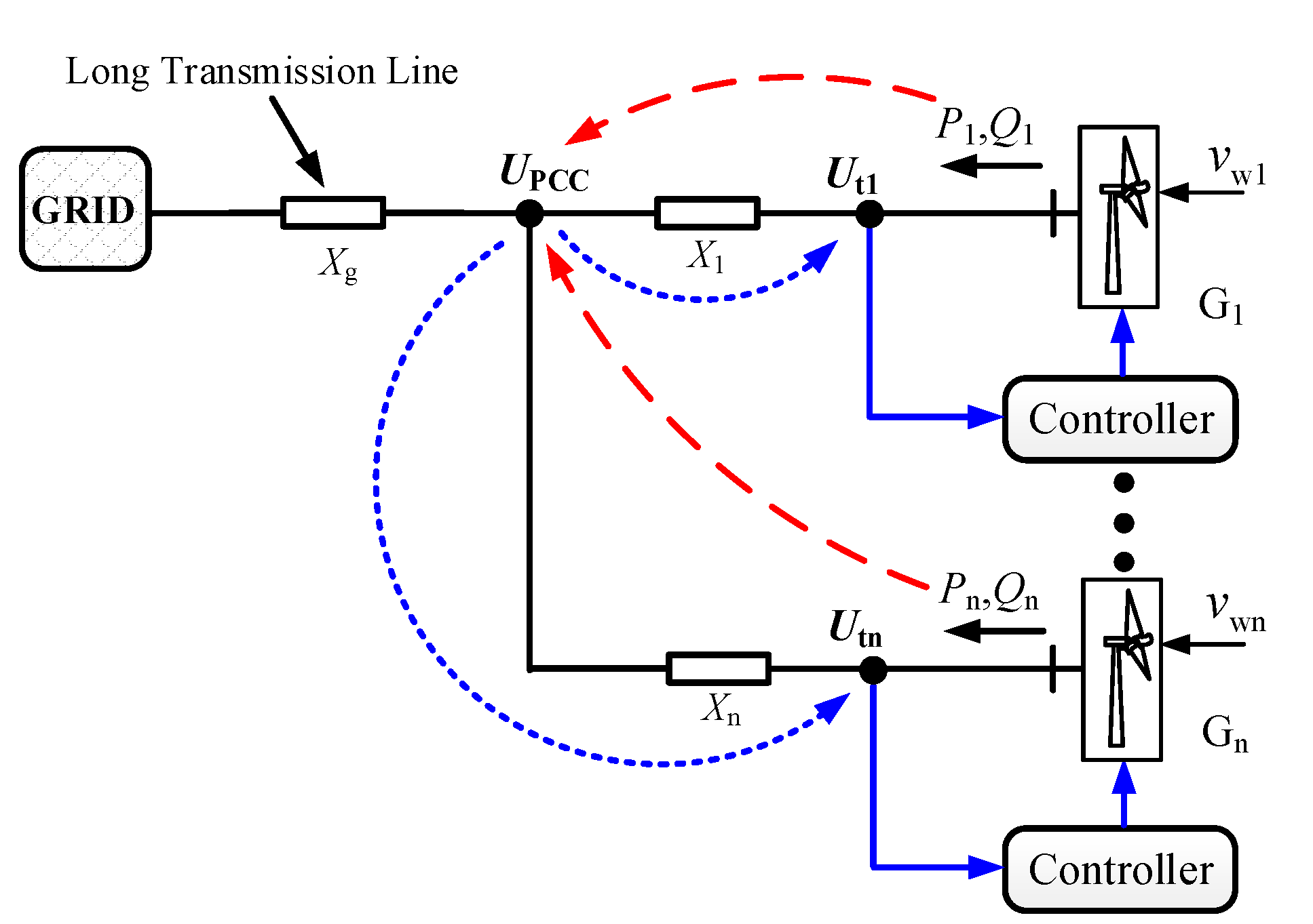
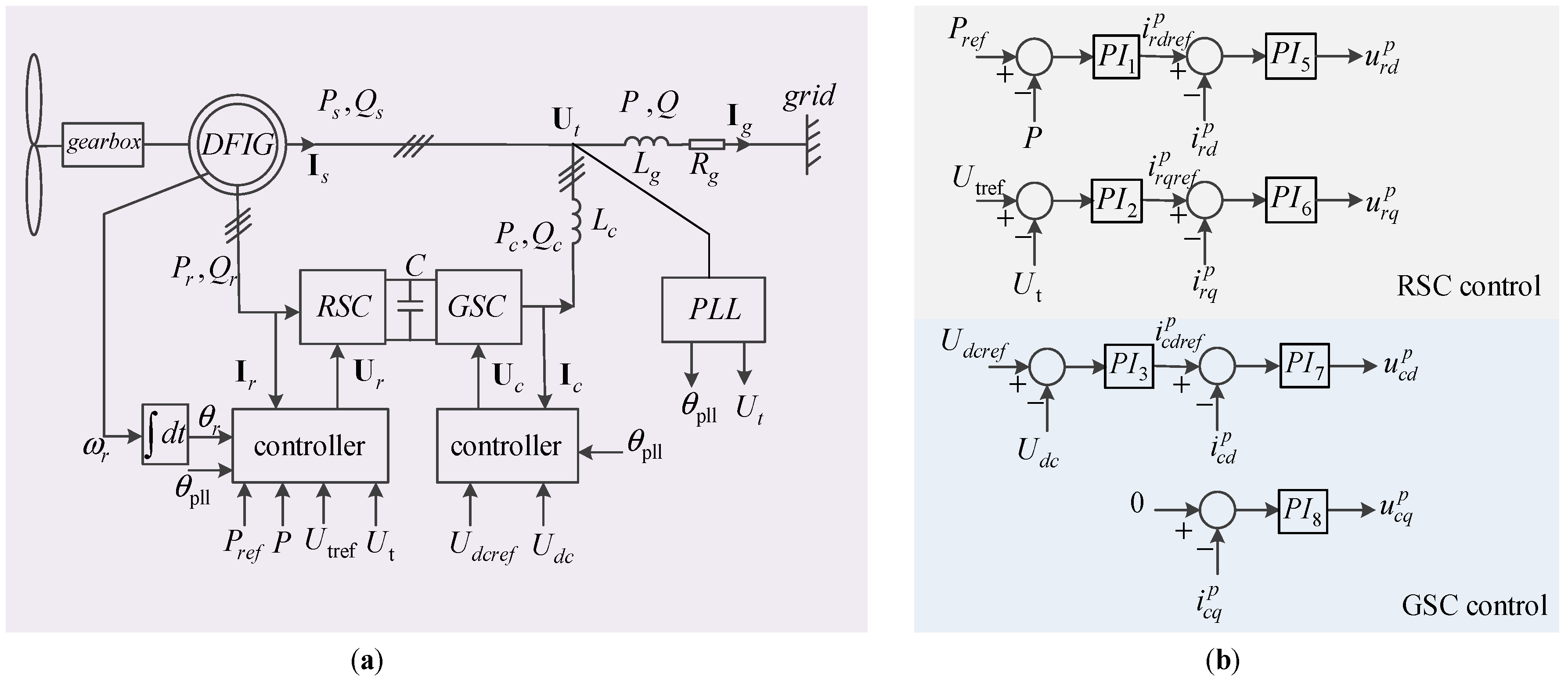
2.1. System Configuration and Multi-WT Interactions

Figure 1 depicts a simplified diagram of a wind farm with multiple radially connected wind turbines (WTs) that were integrated into the bulk power grid. The role of the grid strength on the dynamic interactions among the WTs can be understood, as follows.
As shown in Figure 1, the point of common connection (PCC) voltage acts as a linkage for the interconnection between the WTs and the power grid. A change of PCC voltage will induce the variation of generator’s terminal bus voltage, and then drive the controllers of WT to react and affect its dynamic output powers. In turn, the variations of one WT’s output powers would alter the PCC voltage, thus affecting the terminal bus voltages and output powers of other WTs, and vice versa. In the process above, when the grid impedance is high, the same amount of one generator’s output power fluctuation will cause a larger extent of PCC voltage change, thus bringing a larger effect on other WT’s terminal voltage and output power. Consequently, weaker grid strength will enlarge the level of dynamic couplings among the WTs.

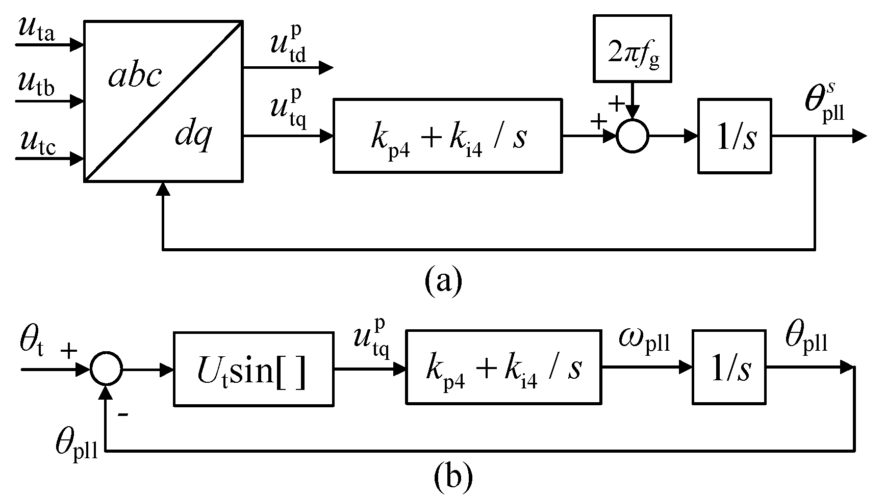
2.2. System Modeling

(1) DFIG System Model:Figure 2 gives the diagram for the typical stator-voltage-oriented vector-controlled DFIG system [14]. The slow turbine dynamics are decoupled from the power grid by the converters, so for the purpose of grid-integration stability investigations, this slow mechanical dynamics are neglected in this paper and a constant power reference Pref is assumed.
The control of DFIG is constructed in the synchronous dq reference frame. Under the synchronous dq reference frame, the voltage and flux equations for machine model are given as
{ U t = R s I s + d ψ s d t + j ω 1 ψ s U r = R r I r + d ψ r d t + j ( ω 1 ω r ) ψ r
{ ψ s = L s I s L m I r ψ r = L m I s L r I r
in which, the stator side uses the generator convention while the rotor side adopts the motor convention.
The associated power and circuit equations can be written as
P r = 1.5   ( u r d i r d + u r q i r q )
P c = 1.5   ( u t d i c d + u t q i c q )
P r P c = C U d c d U d c d t
P = 1.5   ( u t d i g d + u t q i g q )
I g = I s + I c
(2) RSC and GSC Controls: RSC and GSC both contain two cascaded loops. The typical proportional-integral (PI) controllers are implemented in each control loop. The superscript p indicates the dq components of a variable are resolved in the PLL-dq reference frame. For the RSC, the outer active/reactive control loops regulate the active power of the entire generator that was sent to the grid and the terminal bus voltage level, respectively. The GSC utilizes the DC-link voltage control to guarantee the power delivery from the RSC to the grid. Unity power factor control is usually used in the GSC reactive power control channel. The related equations for the DFIG RSC and GSC controls are
i r d r e f p = ( P r e f P ) ( k p 1 + k i 1 s )
i r q r e f p = ( U t r e f U t ) ( k p 2 + k i 2 s )
i c d r e f p = ( U d c r e f U d c ) ( k p 3 + k i 3 s )
u r d p = ( i r d r e f p i r d p ) ( k p 5 + k i 5 s )
u r q p = ( i r q r e f p i r q p ) ( k p 6 + k i 6 s )
u c d p = ( i c d r e f p i c d p ) ( k p 7 + k i 7 s )
u c q p = i c q p ( k p 8 + k i 8 s )
(3) Phase-Locked Loop:Figure 3a gives a typical control scheme of PLL [15]. PLL tracks the phase angle of DFIG terminal bus voltage to realize the synchronization with the power grid. It is worth noting that the input three-phase terminal voltage in Figure 3a can be presented in the synchronous frame with the polar form as Utθt, according to [16], an equivalent form of PLL can be expressed in the synchronous frame, as shown in Figure 3b. The associated equations are
u tq p = U t sin ( θ t θ pll )
θ pll = u tq p ( k p 4 + k i 4 s ) 1 s
The linearized PLL model can be obtained as
Δ θ pll Δ θ t = U t 0 k p 4 s + U t 0 k i 4 s 2 + U t 0 k p 4 s + U t 0 k i 4
(4) Coordinate Transformation: For the control of a DFIG, the d-axis of the synchronous frame is usually selected to align with steady-state terminal bus voltage for the sake of generator local control. The infinite bus voltage is normally assigned as reference for the global coordinate, while assuming the steady-state phase leading of DFIG terminal voltage over the infinite bus voltage is θ0, as depicted in Figure 4, the relations for the components, such as voltages and currents, in the global and local frame can be expressed as
{ f x = f d cos θ 0 f q sin θ 0 f y = f d sin θ 0 + f q cos θ 0
The network circuit equations are given as
U j U i = R i j I i j + j ω 1 I i j L i j
in which, Ui, Uj denote the voltage of node i and j, respectively. Iij represents the current flowing from node i to node j. Rij and Lij are the associated resistance and inductance.
(5) Small-Signal Model for Overall System: Combining all of the equations above for the DFIG subsystem and the power grid, the math model of the overall system can be generated. Linearizing the model around one equilibrium point, the small-signal model in the canonical state-space form can be expressed as
Δ x ˙ = A Δ x + B Δ u
Δ y = C Δ x + D Δ u
where Δx represents the state variables associated with the machine dynamics and control dynamics of each DFIG, Δu can be the reference signals, including ΔPref, ΔUtref, and ΔUdcref, while the output vector Δy is selected as ΔPr, ΔUt, ΔUdc in this paper. The eigenvalues and eigenvectors can be obtained from the state matrix A, and they will be used for the following analysis.

3. Eigenvalue Sensitivity Analysis

Based on the proposed small-signal model, this section presents eigenvalue sensitivity analysis to identify the dominant oscillatory modes and possible instabilities. The impact of grid strengths and operating points will be examined. For simplicity of analysis, a system that is composed of two 2-MW DFIGs in parallel connection to a grid (see the configuration in Figure 1) is studied. The control and machine parameters of the two DFIGs are identical and given in the Appendix A, in which the PI gains of DFIG controllers are mainly referred to the demo model in Matlab [17].

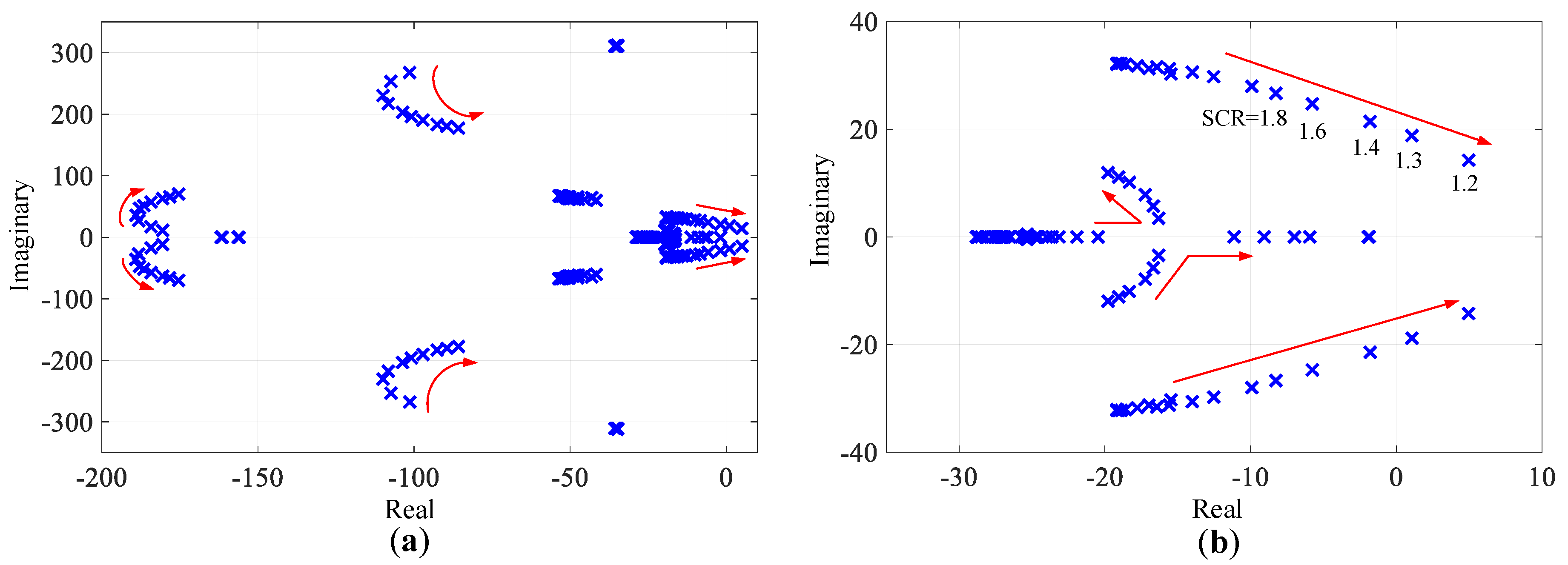
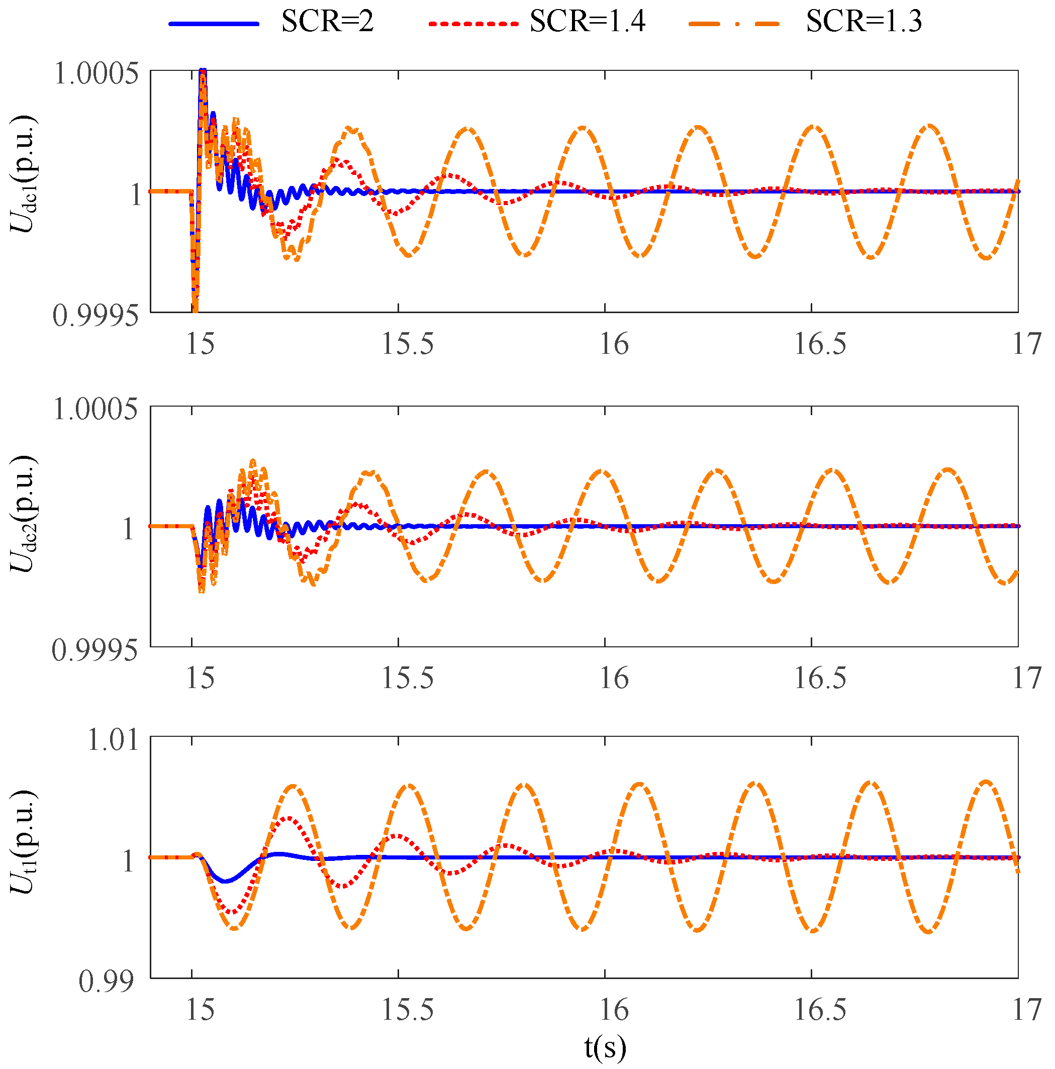
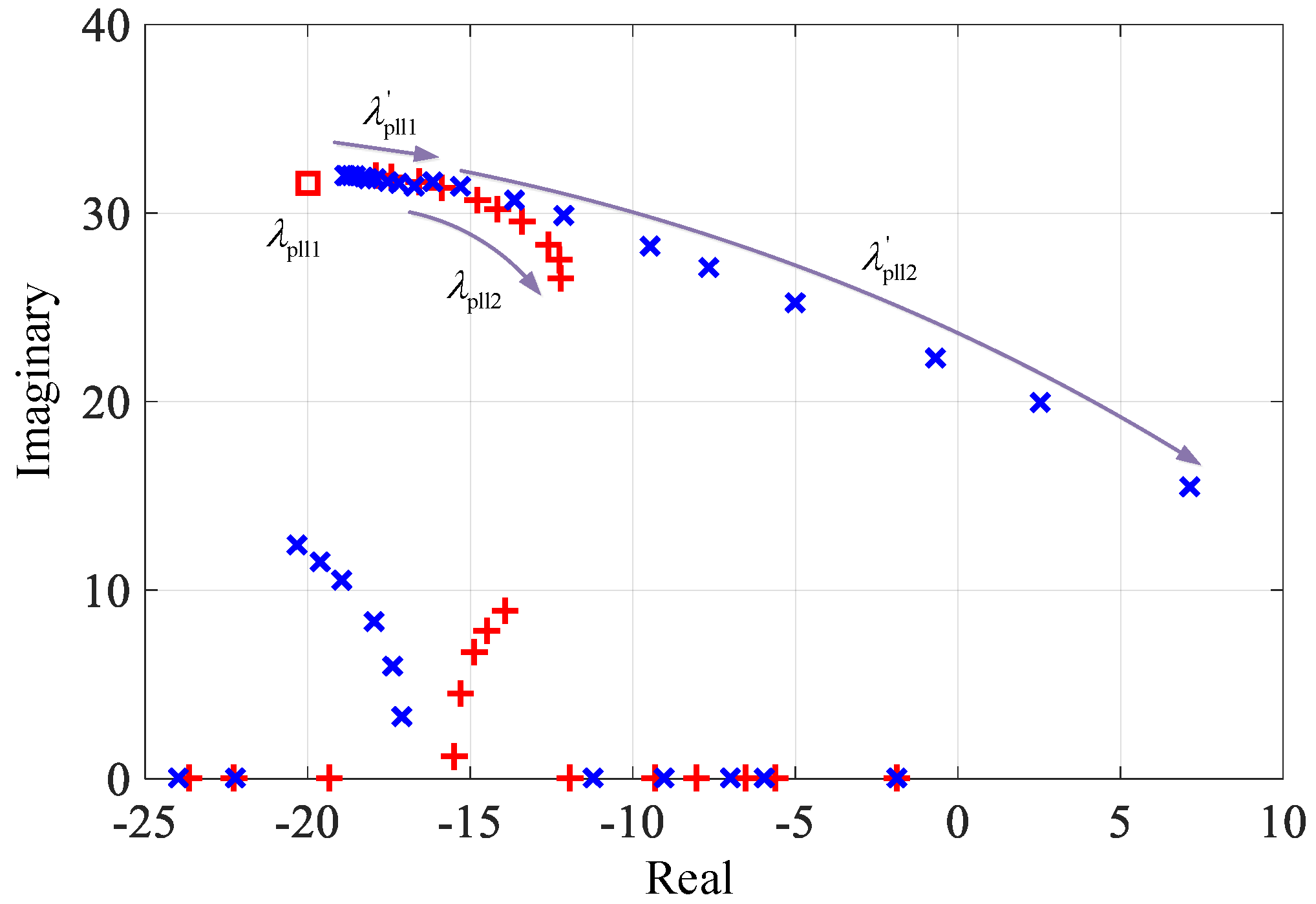
3.1. The Impact of Grid Strengths

A weak grid connection is known to threaten the stability of wind generations. Generally, the short circuit, as the measurement of the grid strength, is defined as SCR =   U pcc 2 /(XlPwf) [18], where Upcc and Pwf denote the PCC voltage and rated power of the wind farm, respectively. In this subsection, it is assumed that the two DFIGs output nominal power, i.e., P1 = P2 = 1 p.u., and the impact of grid strength is checked by gradually increasing the grid impedance. The line resistance is set as Rl = 0.1 Xl.
Figure 5a gives the locus for the main pairs of eigenvalues when the SCR reduces from 5.0 to 1.2. It is shown that the majority of these modes have sufficient damping in this process, except that there is a pair of complex eigenvalues that move from the left-half plane to the right-half plane with the decrease of grid strength. This pair of eigenvalues are the dominant mode of this system. A closer look, as given in Figure 5b, shows that the marginal instability occurs when SCR decreases from 1.4 to 1.3. Meanwhile, the angular frequency of this mode slightly declines with the decrease of SCR, which ranges around 30 rad/s to 18 rad/s.

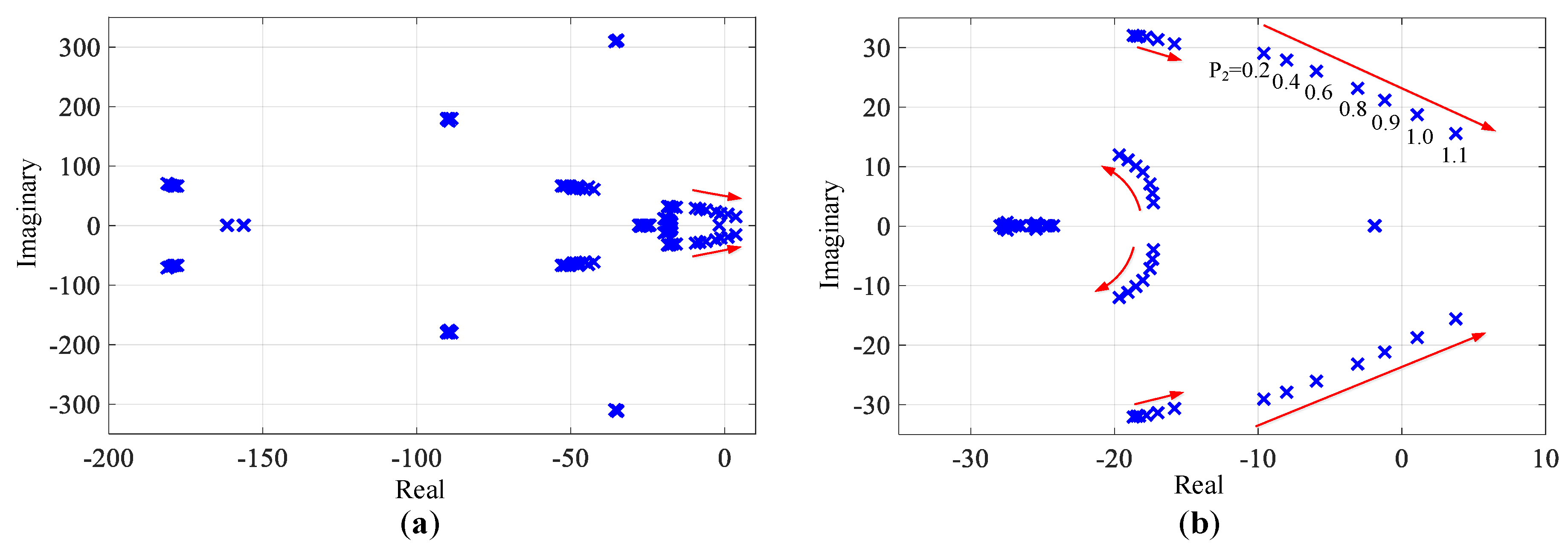
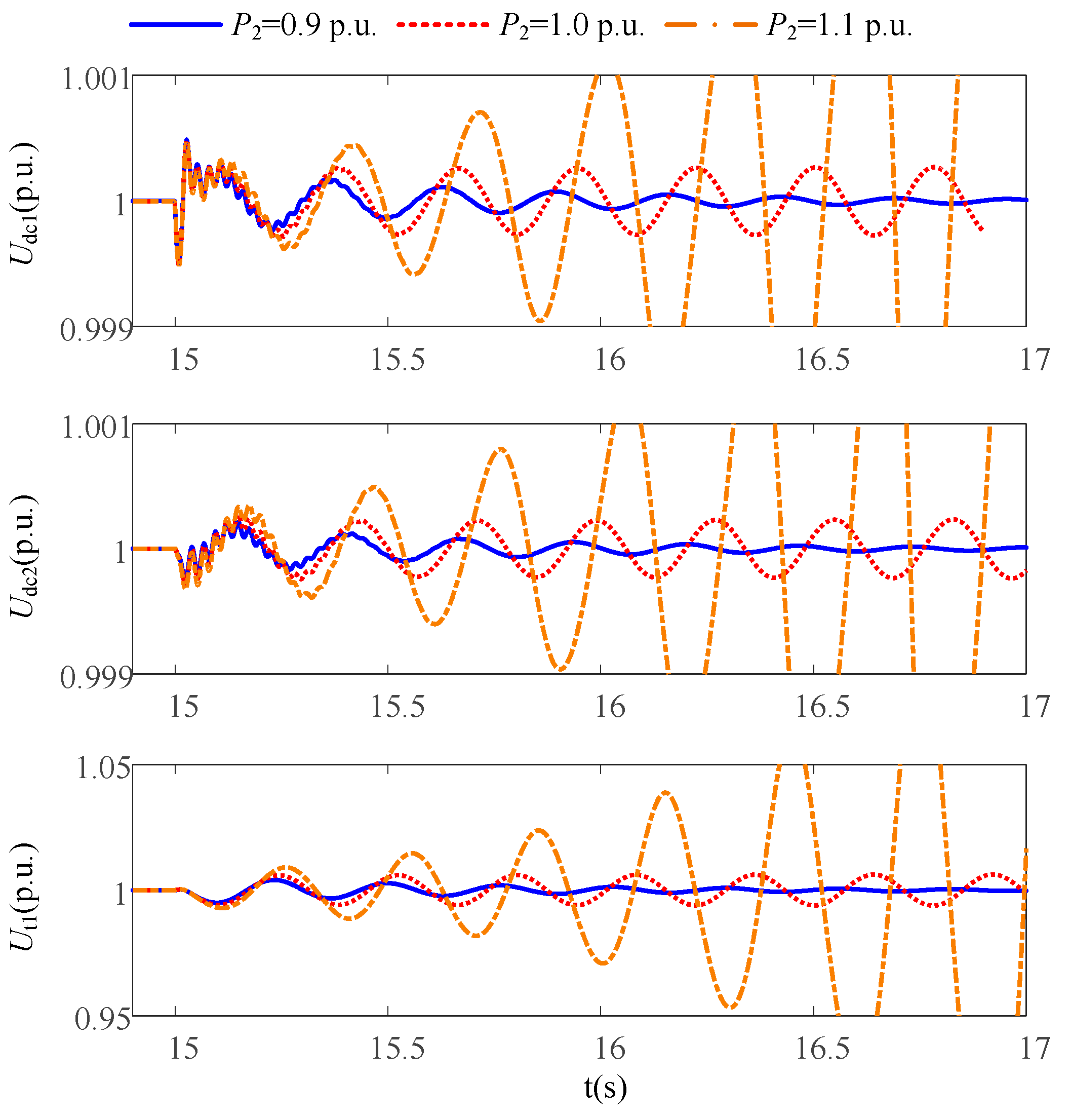
3.2. The Impact of Operating Points

The impact of operating points on stability is also investigated. The SCR is set as 1.3, the output power of G1 is fixed to 1 p.u., while G2 output power varies from 0.2 p.u. to 1.1 p.u. Figure 6a depicts the corresponding eigenvalue locus. When compared to Figure 5, a similar finding is that the same pair of complex eigenvalues is the most sensitive mode to G2’s power change, and it gets unstable with P2 increase; while the rest system modes are more insensitive with adequate damping. A zoom in look, as given in Figure 6b, shows that instability happens when P2 varies from 0.9 p.u. to 1.0 p.u.

3.3. Participation Factor Analysis

Participation factor is a useful tool in eigenvalue analysis, and it is defined as [19]
p k i = ϕ k i ψ i k
where ϕ k i , ψ i k are the kth entry of the right and left eigenvector, respectively. Participation factor, as given in (22), is a measure of the relative participation degree of the kth state variable in the ith mode. When considering normalized eigenvector, the sum of the participation factors to any mode for each state variable is equal to 1. Meanwhile, the dynamics of a state variable are directly affected by the associated controls, e.g., DC-link voltage control significantly contributes to the dynamic state of DC-link voltage. Accordingly, this section utilizes participation factor analysis to explore the correlated state variables and controls to system critical modes.
The operating condition is set as the same as the case in Section 3.1. Two different grid strength conditions, SCR = 4 and SCR = 1.4, are compared. Corresponding participation factor analysis results for the two pair of complex eigenvalues that are located close to the imaginary axis are shown in Table 1 and Table 2, respectively. For SCR = 4, the results in Table 1 show that the dominant mode is mainly governed by the PLL controls of the two DFIGs, and the share of participation for the two DFIGs are nearly equal. This indicates that the interactions between the PLLs of the two generators play a crucial role in system stability. For SCR = 1.4, PLL still accounts for a large contribution on the dominant mode, while the participation level of RSC active/reactive power controls also gets noticeable. This implies that the coupling between PLL and DFIG RSC power controls also becomes stronger under weak grid conditions. In the meanwhile, other different operating scenarios covering a moderate range of variations of generator output powers, grid strengths, and control parameters are also examined. Due to space limitation, the detailed results are not presented here. Nevertheless, one point in common for these case studies that should be clarified is that the above PLL related mode always dominates system stability, and both WT output power increase and grid strength decrease will deteriorate the damping of this mode.

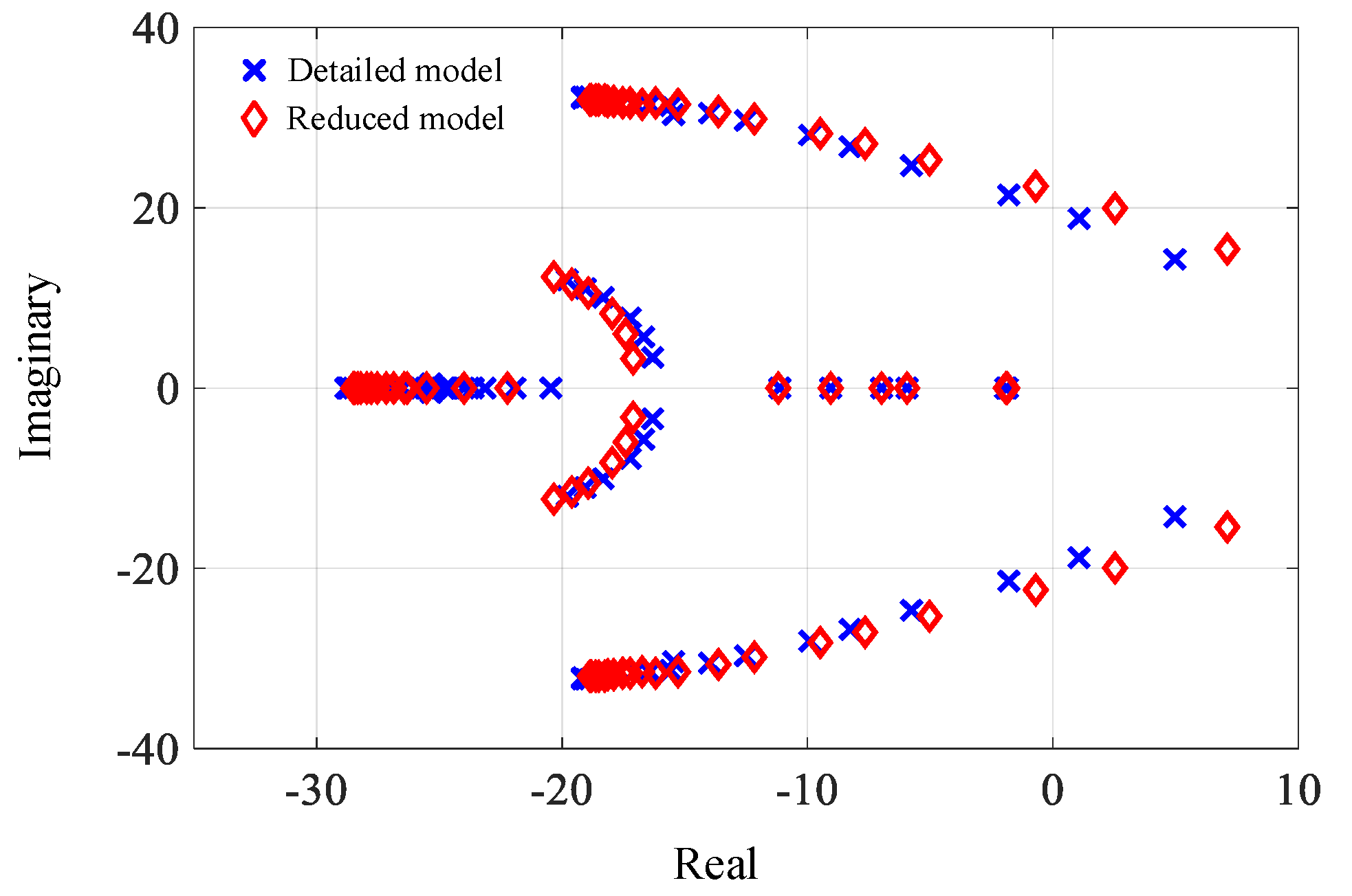
4. Proposed Reduced-Order Model

In the section above, participation factor analysis identifies that the dominant mode is mainly participated by the PLL related state variables, and is also partially contributed by the RSC active/reactive power controls associated states under weak grid conditions. However, other system state variables hardly take part in this mode, and their correlated modes lie far to the imaginary axis, exhibiting a decoupling with this dominant mode. Generally, this is reasonable due to the bandwidths of RSC power controls and PLL being normally designed slower than the RSC inner current controls and GSC controls.
Due to this decoupling, it is possible to reduce the original detailed mode while still preserving the dominant oscillatory behaviors. We make the following assumptions for model reductions: (1) The machine dynamics are omitted by assuming d Ψs/dt = 0, d Ψr/dt = 0 in Equation (1); (2) The dynamics of RSC current controls are neglected by assuming that the current can instantaneously track the reference, i.e., i rd p = i rdref p and i rq p = i rqref p ; (3) The DC voltage dynamics and fast GSC controls are neglected by assuming the RSC power to be equal to the GSC power, namely, Pc = Pr.
Accordingly, the reduced order model only preserves the dynamics of RSC power controls and PLL, each DFIG model is greatly reduced to a four-order subsystem. The eigenvalues of the detailed model and reduced model are compared to validate the feasibility of this simplification. Table 3 gives the comparison results at the operating condition P1 = P2 = 1 p.u., SCR = 2, in which, for the detailed model, only the part of eigenvalues that are close to the eigenvalues of the reduced model are listed. The results demonstrate that the calculated eigenvalues from the reduced model are quite close to the ones from the detailed model. In addition, Figure 7 compares and shows varied grid strength conditions (with the same setting in Section 3.1). It shows that, in the relative grid strength condition, the eigenvalues for the two models almost coincide with each other; while for the very weak grid condition (SCR around 1.4), there is a very slight difference for the two cases. Overall, it can be concluded that the reduced-order model can maintain the primary oscillatory modes of the detailed model well. Owing to its simplicity, it is more readily to make out the instability causes from the reduced model.

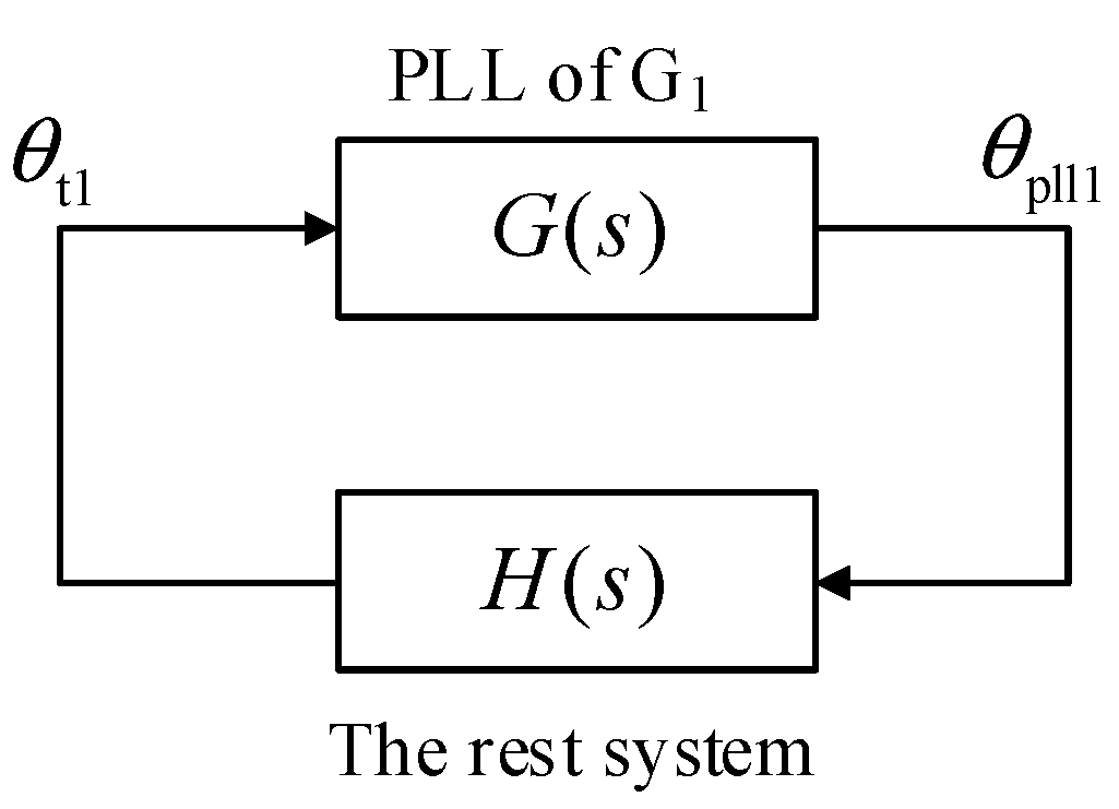
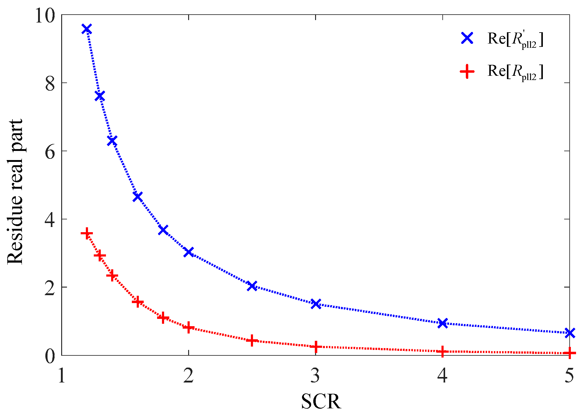
5. Residue-Based Explanation on Weak-Grid Instability

This section gives a further explanation for understanding the identified instability under weak grid conditions in terms of residues. The proposed reduced-order model is utilized for the analysis herein.

5.1. Transfer Function Residue

Given a transfer function Fij(s) from the input ui and the output yi, it can always be expressed as a sum of partial fractions in the following form
F i j ( s ) = y i ( s ) u i ( s ) = k = 1 n R k s λ k + d i j
in which, Rk is the residue corresponding to eigenvalue λk, and it measures the sensitivity of λk to a scalar feedback [20]. The residue is a complex number, which can be described in the complex plane as depicted in Figure 8. For λk, the angle of residue Rk gives the direction, as shown in Figure 8, of how the locus of λk will go, while the magnitude of residue Rk indicates the extent of the movement of λk. How to derive the residues from a transfer function is detailed in [19]. For different input-output pairs, the residues for the same eigenvalue of a system are different. Therefore, the magnitudes of residue, which indicate how much an eigenvalue will be affected for a particular input-output signal path, are useful for the signal selections in feedback control design. As a typical application, residues have been utilized in power oscillation damping controls [21,22,23].

5.2. Explanation on Weak-Grid Instability

Participation factor analysis in Section 3.3 indicates that instability at weak grid conditions is highly related to the interactions between the PLL modes of the two generators. We can express the closed loop system as two subsystems interconnected, as shown in Figure 9, in which the forward term G(s) denote the transfer function of PLL in G1, while the feedback term H(s) represents the transfer function of the rest system, to further explore how the two PLL modes interact to make system unstable. As aforementioned, since the variation of a residue can provide clues regarding the movement of the corresponding mode on the complex plane, the impact of modal interactions within the two subsystems can be assessed by the changes of residues due to the interconnection.
Similar to Equation (23), G(s) and H(s) can be expressed as
G ( s ) = θ pll 1 ( s ) θ t 1 ( s ) = R pll 1 s λ pll 1 + i = 1 m R i s λ i + d g
H ( s ) = θ t 1 ( s ) θ pll 1 ( s ) = R pll 2 s λ pll 2 + j = 1 n R j s λ j + d h
in which, λpll1, λpll2 represents the PLL modes of the two open-loop subsystems and Rpll1 and Rpll2 are the corresponding residues.
To assess the modal interaction within the two subsystems, generally, we can evaluate the impact of mode i in G(s) on the residue of mode j in H(s), as
R j = R j R i λ j λ i
Equation (26) shows that when λi and λj are close, their interaction tends to be stronger for the larger effect on the gain of the residue. This preliminarily answers why PLL mode in G1 tightly couples with the PLL mode in G2.
Figure 10 provides the eigenvalue locus for the two open-loop subsystems and the closed-loop overall system when SCR varies from 5 to 1.2 (Same with the case in Section 3.1). In which, λ pll 1 and λ pll 2 represent the two PLL modes of the closed-loop system. A distinct feature that is given in Figure 10 is that, with the reduction of SCR, the open-loop PLL mode of G2 λ pll 2 slightly shifts to the right, while the corresponding closed-loop mode λ pll 2 experiences a much more dramatic right movement, and it even crosses the imaginary axis. This difference comes from the interaction with G1 PLL mode, and the change of residue of G2 PLL mode due to the interaction with G1 PLL mode can be expressed at the complex frequency λ pll 2 , as
R pll 2 = R pll 2 R pll 1 λ pll 2 λ pll 1
in which, R pll 2 denotes the residue that is associated with the closed-loop G2 PLL mode.
We can compare the value of R pll 2 and R pll 2 to examine the level of movement of the open-loop and closed-loop PLL mode of G2. Figure 11 depicts the real parts of the two residues for SCR that varies from 5 to 1.2. Noting that the real part of a residue is positive indicates that the associated mode moves rightwards in the horizontal direction if the selected input-output channel subjected to a unity feedback. With the inclusion of the interaction with PLL mode of G1, it can find that Re [ R pll 2 ] is always larger than Re [ R pll 2 ] , which implies the larger size of right movement of the closed-loop PLL mode of G2 as compared to the open-loop case. This result is in good agreement with the root locus in Figure 10. Meanwhile, Re [ R pll 2 ] > Re [ R pll 2 ] also demonstrates that the interaction of the two PLL modes is always detrimental for closed-loop stability. In addition, the value of Re [ R pll 2 ] sharply increases with grid strength decline for SCR < 2, which indicates the aggravated deterioration of system stability. Hence, the tendency of residue change can be regarded as a precursor of instability to some extent.

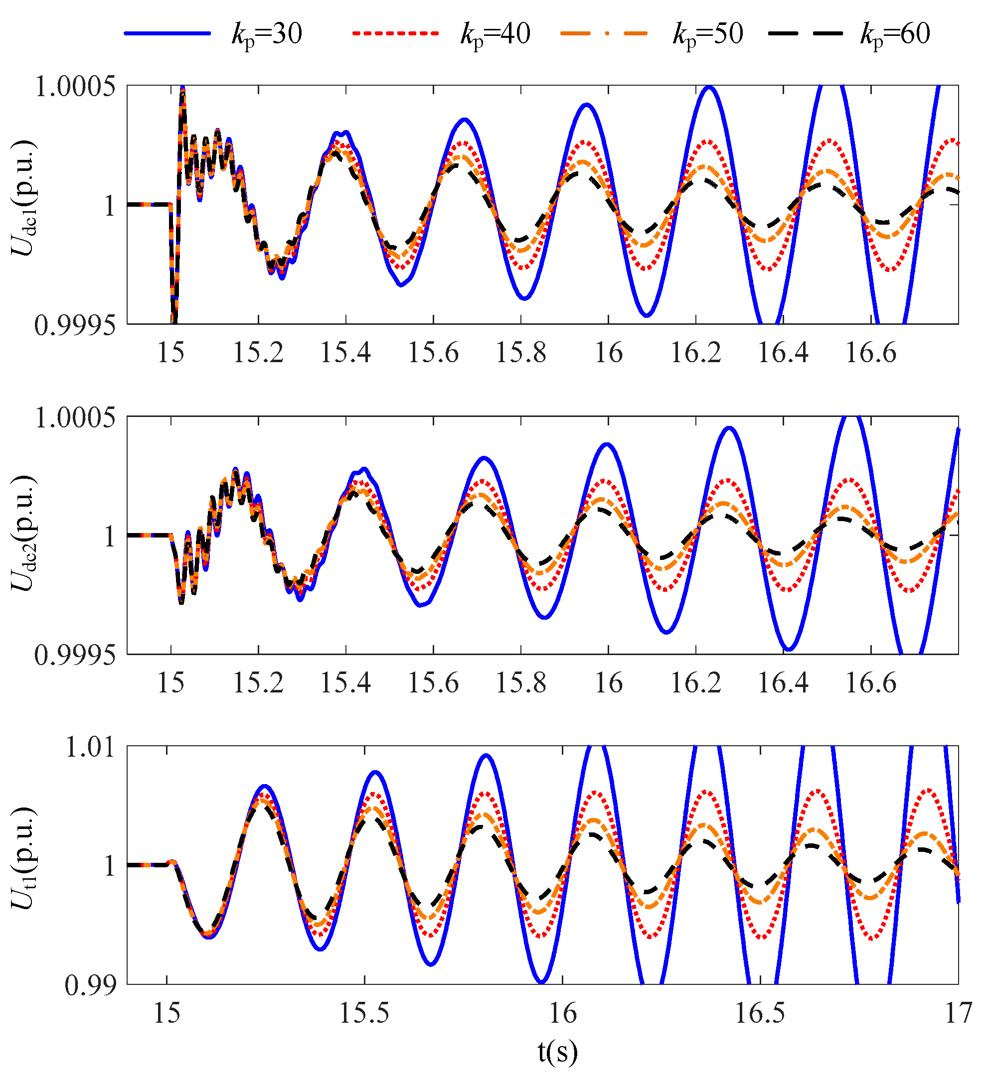
6. Simulation Studies

To validate the analysis above, a detailed model comprised of two 2MW DFIG-based wind turbines in parallel connection to a weak grid is constructed in Matlab/Simulink. For system configuration, refer to Figure 1, and the parameters are identical with the aforementioned analyses cases. For all of the simulation cases, the pre steady state is achieved by proper tuning of control parameters, and at t = 15 s, the tuned controller parameters are restored to the initial values (as given in the Appendix A) and a small disturbance with a 0.01 p.u. step up of G1 active power reference is subjected. The responses of DC-link voltages in G1 and G2, and terminal bus voltage in G1 are recorded.
The impact of grid strengths is examined and the conditions are set the same with the case in Section 3.1. Figure 12 gives the results at SCR = 2, 1.4 and 1.3. It shows that system stability gets worse with the decline of grid strength, the marginal instability happens around SCR = 1.3. These results are in close consistence with the eigenvalue locus results that are given in Figure 5 and Figure 7. Likewise, given SCR = 1.3, the impact of output power variations of G2 is also checked. Figure 13 shows that increased wind power decreases the system’s stability, and sustained oscillation occurs when P2 varies from 0.9 p.u. to 1.0 p.u. The simulation results are also in well accordance with the eigenvalue analysis in Section 3.2.
Eigenvalue participation factor analysis in Section 3.3 identifies that the dominant mode for the loss of stability in weak grids is highly related to the interactions between the PLL controls of the two generators. Further, the residue-based analysis in Section 5.2 demonstrates that the interaction of the two PLL modes is always detrimental for closed-loop stability. Transparently, one feasible countermeasure to enhance system stability is to weaken the interaction of the two PLL modes. As indicated in Equation (27), one of the possible ways of reducing the mode coupling is to separate the locations of the two open-loop modes in the complex plane. As depicted in Figure 10, to diminish the negative interaction impact of λ pll 1 on λ pll 2 , a simple way is to left shift the open-loop mode λ pll 1 . As the left movement of λ pll 1 has no effect on the open-loop mode λ pll 2 , but it weakens the interaction with λ pll 2 , so the damping of the closed-loop dominant mode λ pll 2 can be enhanced. Equation (17) shows that the increase of the proportional gain of PLL controllers can realize this objective. Figure 14 gives the simulation validations; the operating condition is set as: P1 = P2 = 1 p.u., SCR = 1.3, varied proportional gains of PLL in G1 is checked. The results confirm the analysis above, the increase of PLL proportional gain can enlarge the damping of the dominant mode, and sustained oscillation gets dampened. Hence, the residue-based analysis can provide some guidance on parameter tunings of a subsystem to improve the closed-loop stability of the overall system, such analysis from the perspective of subsystem interactions can relieve the computation burden instead of directly analyzing the entire closed-loop system, in particular when the scale of the studied system is large.

7. Conclusions

This work studies the synchronization stability of a system that is composed of two DFIGs that are connected in parallel to a weak AC grid. Based on eigenvalue sensitivity and participation factor analysis, the interactions between the synchronization units, i.e., PLLs, of the two WTs, are found as the major culprit of the weak-grid instability. A residue-based analysis is also provided for understanding such instability, which demonstrates that the interactions between PLLs are always detrimental for closed-loop stability, and a weak grid condition will aggravate this interaction. Additionally, increasing the proportional gain of PLL controllers is recommended as a feasible way to improve system stability under weak grid conditions. In terms of analysis methodology, the combination of participation factor analysis and transfer function residue analysis is promising to be applied for studying the stability of larger-scale practical systems, where the former method can be used to locate the dominant modes and identify the remarkable modal interactions, while the latter helps to understand the mechanism of interactions and instability origins.

Author Contributions

Conceptualization, D.W.; methodology, D.W. and Y.H.; software, D.W.; validation, D.W.; investigation, Y.H. and X.D.; writing-original draft preparation, D.W.; writing-review and editing, D.W., Y.H., M.L. and X.D.; supervision, Y.H. and G.Z.; project administration, Y.H.; funding acquisition, Y.H.

Funding

This work is supported by National Natural Science Foundation of China under Grant 51607130.

Conflicts of Interest

The authors declare no conflict of interest.

Nomenclature

Ls, Lr, LmStator, rotor and mutual inductances
Lls, LlrStator and rotor leakage inductances
Rs, RrStator and rotor resistances
ω1, ωrSynchronous and rotor angular frequency
Ut, θtTerminal voltage magnitude and phase
Ps, QsStator active and reactive powers
Pr, QrRotor active and reactive powers
Pc, QcGrid-side converter active and reactive powers
Pi, QiActive and reactive powers sent to grid by generator i
Uc, UrOutput voltage of grid-side converter and rotor-side converter
Is, Ir, IcStator, rotor and grid-side converter current
Ψs, ΨrStator and rotor flux
LcFilter inductance of grid-side converter
θpll, ωpllPLL output angle and frequency
Udc, CDC-link voltage and capacitance
PCCPoint of common connection
kp, kiProportion and integral control gain
LgTransmission line inductance between the PCC and the infinite bus
LiEquivalent line inductance between generator terminal bus and the PCC
Subscripts:
0Steady-state value
d, qSynchronous rotating reference frame signal d-axis and q-axis components
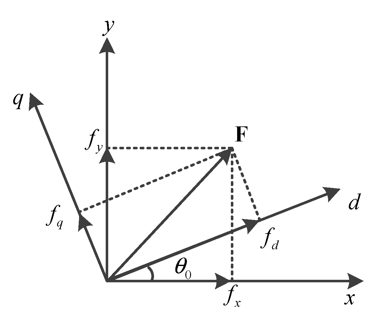
x, yGlobal reference frame signal x-axis and y-axis components
s, rStator and rotor components
refReference signal
Superscript:
pComponents in PLL rotating frame

Appendix A

2-MW DFIG parameters:
Sbase = 2 MWUbase = 690 V(phase to phase RMS value)
ωbase = 2 πfbasefbase = 50 HzRs = 0.022 p.u.Rr = 0.009 p.u.
Lls = 0.171 p.u.Llr = 0.156 p.u.Lm = 3.9 p.u.Lc = 0.3 p.u.
Udcref = 1200 VC = 0.02 FUg = 1 p.u.Rg = 0.1 ω1Lg
Circuit parameters:
L1 = 0.2 p.u., L2 = 0.15 p.u.
Controllers parameters values (p.u.):
RSC active power controlkp1 = 0.4ki1 = 40
RSC terminal voltage controlkp2 = 0.25ki2 = 25
DC-link voltage controlkp3 = 1.5 ki3 = 100
Phase-locked loopkp4 = 40ki4 = 1400
RSC current controlkp5 = kp6 = 0.6ki5 = ki6 = 80
GSC current controlkp7 = kp8=8ki7 = ki8 = 200

References

  1. Zhou, J.Z.; Gole, A.M. VSC transmission limitations imposed by AC system strength and AC impedance characteristics. In Proceedings of the 10th IET International Conference on AC and DC Power Transmission (ACDC), Birmingham, UK, 4–5 December 2012; pp. 1–6. [Google Scholar]
  2. Yang, D.; Wang, X.; Liu, F.; Xin, K.; Liu, Y.; Blaabjerg, F. Adaptive reactive power control of PV power plants for improved power transfer capability under ultra-weak grid conditions. IEEE Trans. Smart Grid 2019, 10, 1269–1279. [Google Scholar] [CrossRef]
  3. Wang, L.; Xie, X.; Jiang, Q.; Liu, H.; Li, Y.; Liu, H. Investigation of SSR in practical DFIG-based wind farms connected to a series-compensated power system. IEEE Trans. Power Syst. 2015, 30, 2772–2779. [Google Scholar] [CrossRef]
  4. Huang, S.H.; Schmall, J.; Conto, J.; Adams, J.; Zhang, Y.; Carter, C. Voltage control challenges on weak grids with high penetration of wind generation: Ercot experience. In Proceedings of the IEEE Power Energy Social General Meeting, San Diego, CA, USA, 22–26 July 2012; pp. 1–7. [Google Scholar]
  5. Harnefors, L.; Bongiorno, M.; Lundberg, S. Input-admittance calculation and shaping for controlled voltage-source converters. IEEE Trans. Ind. Electron. 2007, 54, 3323–3334. [Google Scholar] [CrossRef]
  6. Messo, T.; Jokipii, J.; Mäkinen, A.; Suntio, T. Modeling the grid synchronization induced negative-resistor-like behavior in the output impedance of a three-phase photovoltaic inverter. In Proceedings of the IEEE Fourth International Symposium on Power Electron, For Distributed Generations System, Rogers, AR, USA, 8–11 July 2013; pp. 1–8. [Google Scholar]
  7. Wang, D.; Liang, L.; Shi, L.; Hu, J.; Hou, Y. Analysis of modal resonance between PLL and DC-link voltage control in weak-grid tied VSCs. IEEE Trans. Power Syst. 2019, 34, 1127–1138. [Google Scholar] [CrossRef]
  8. Hu, J.; Huang, Y.; Wang, D.; Yuan, H.; Yuan, X. Modeling of grid connected DFIG-based wind turbines for DC-link voltage stability analysis. IEEE Trans. Sustain. Energy 2015, 6, 1325–1336. [Google Scholar] [CrossRef]
  9. Zhang, L.; Harnefors, L.; Nee, H.P. Power-synchronization control of grid-connected voltage-source converters. IEEE Trans. Power Syst. 2010, 25, 809–820. [Google Scholar] [CrossRef]
  10. Wang, S.; Hu, J.; Yuan, X. Virtual synchronous control for grid-connected DFIG-based wind turbines. IEEE J. Emerg. Sel. Top. Power Electron. 2015, 3, 932–944. [Google Scholar] [CrossRef]
  11. Wen, B.; Dong, D.; Boroyevich, D.; Burgos, R.; Mattavelli, P.; Shen, Z. Impedance-based analysis of grid-synchronization stability for three-phase paralleled converters. IEEE Trans. Power Electron. 2016, 31, 26–38. [Google Scholar] [CrossRef]
  12. Rosso, R.; Andresen, M.; Engelken, S.; Liserre, M. Analysis of the interaction among power converters through their synchronization mechanism. IEEE Trans. Power Electron. 2019, 34, 12321–12332. [Google Scholar] [CrossRef]
  13. Huang, Y.; Wang, D.; Shang, L.; Zhu, G.; Tang, H.; Li, Y. Modeling and stability analysis of DC-link voltage control in multi VSCs with integrated to weak grid. IEEE Trans. Energy Convers. 2017, 32, 1127–1138. [Google Scholar] [CrossRef]
  14. Akagi, H.; Sato, H. Control and performance of a doubly-fed induction machine intended for a flywheel energy storage system. IEEE Trans. Power Electron. 2002, 17, 109–116. [Google Scholar] [CrossRef]
  15. Gole, A.; Sood, V.K.; Mootoosamy, L. Validation and analysis of a grid control system using D-Q-Z transformation for static compensator system. In Proceedings of the Canadian Conference on Electrical and Computer Engineering, Montreal, PQ, Canada, 17–20 September 1989; pp. 745–748. [Google Scholar]
  16. He, W.; Yuan, X.; Hu, J. Inertia provision and estimation of PLL-based DFIG wind turbines. IEEE Trans. Power Syst. 2017, 32, 510–521. [Google Scholar] [CrossRef]
  17. Wind Farm-DFIG Detailed Model, MATLAB Simulink. Available online: https://uk.mathworks.com/help/physmod/sps/examples/wind-farm-dfig-detailed-model.html (accessed on 8 October 2019).
  18. Zhou, J.; Ding, H.; Fan, S. Impact of short-circuit ratio and phase-locked-loop parameters on the small-signal behavior of a VSC-HVDC converter. IEEE Trans. Power Deliv. 2014, 29, 2287–2296. [Google Scholar] [CrossRef]
  19. Kundur, P. Power System Stability and Control; The EPRI Power System Engineering Series; McGraw-Hill: New York, NY, USA, 1994. [Google Scholar]
  20. Rogers, G. Power System Oscillations; Kluwer Academic Publishers: New York, NY, USA, 2000. [Google Scholar]
  21. Heniche, A.; Kamwa, I. Assessment of two methods to select wide-area signals for power system damping control. IEEE Trans. Power Syst. 2008, 23, 572–581. [Google Scholar] [CrossRef]
  22. Pagola, F.L.; Perez-Arriaga, I.J.; Verghese, G.C. On sensitivities residues and participations: Applications to oscillatory stability and control. IEEE Trans. Power Syst. 1989, 14, 278–285. [Google Scholar] [CrossRef]
  23. Morato, J.; Knüppel, T.; Østergaard, J. Residue-based evaluation of the use of wind power plants with full converter wind turbines for power oscillation damping control. IEEE Trans. Sustain. Energy 2014, 5, 82–89. [Google Scholar] [CrossRef]
Figure 1. Simplified diagram of a radially connected wind farm integrated into the power grid.
Energies 12 04361 g001
Figure 2. A grid-tied vector-controlled doubly-fed induction generator (DFIG)-based wind generator system. (a) System main diagram; (b) rotor side converter (RSC) and grid-side converter (GSC) controls.
Energies 12 04361 g002
Figure 3. Block diagram of phase-locked loop (PLL) model: (a) the real structure of the PLL, (b) equivalent representation in synchronous reference frame.
Energies 12 04361 g003
Figure 4. Relationships for the components between the global frame and the local frame.
Energies 12 04361 g004
Figure 5. Eigenvalue locus for short-circuit ratio (SCR) varying from 5 to 1.2 at the condition P1 = P2 = 1 p.u. (a) Locus for major pairs of eigenvalues; and, (b) A zoom in look for dominant eigenvalues.
Energies 12 04361 g005
Figure 6. Eigenvalue locus for P2 varying from 0.2 p.u. to 1.1 p.u. at the condition P1 = 1 p.u. and SCR = 1.3. (a) Locus for major pairs of eigenvalues, (b) A zoom in look for dominant eigenvalues.
Energies 12 04361 g006
Figure 7. Eigenvalue comparisons between reduced- and full-order model for SCR varying from 5 to 1.2.
Energies 12 04361 g007
Figure 8. Residue indicated eigenvalue sensitivity.
Energies 12 04361 g008
Figure 9. System closed-loop representation by a PLL subsystem interconnected with the rest system.
Energies 12 04361 g009
Figure 10. Locus of open-loop and closed-loop PLL modes for SCR varying from 5 to 1.2.
Energies 12 04361 g010
Figure 11. Real parts of the residues that are associated to the open-loop and closed-loop PLL mode of G2 under varied grid strengths.
Energies 12 04361 g011
Figure 12. The responses of DC-link voltage and terminal bus voltage with varied grid strengths at P1 = P2 = 1 pu.
Energies 12 04361 g012
Figure 13. The responses of DC-link voltage and terminal bus voltage with varied output powers of G2 at P1 = 1 p.u. and SCR = 1.3.
Energies 12 04361 g013
Figure 14. The responses of DC-link voltage and terminal bus voltage with varied PLL proportional gains in G1.
Energies 12 04361 g014
Table 1. Participation factors of λ1,2 and λ3,4 at SCR = 4.
EigenvalueParticipating FactorsRelated Controls
λ1,2−15.409 ± j31.153 Δ ω pll 1   =   0.227 ,   Δ θ pll 1 = 0.261G1 PLL
Δ ω pll 2   =   0.238 ,   Δ θ pll 2 = 0.245G2 PLL
λ3,4−19.183 ± j32.153 Δ ω pll 1   =   0.248 ,   Δ θ pll 1 = 0.243G1 PLL
Δ ω pll 2   =   0.232 ,   Δ θ pll 2 = 0.259G2 PLL
Table 2. Participation factors of λ1,2 and λ3,4 at SCR = 1.4.
EigenvalueParticipating FactorsRelated Controls
λ1,2−1.812 ± j21.389 Δ i rdref 1 p   =   0.051 ,   Δ i rqref 1 p = 0.105G1 RSC P and Q
Δ ω pll 1   =   0.170 ,   Δ θ pll 1 = 0.180G1 PLL
Δ i rdref 2 p   =   0.048 ,   Δ i rqref 2 p = 0.107G2 RSC P and Q
Δ ω pll 2   =   0.168 ,   Δ θ pll 2 = 0.179G2 PLL
λ3,4−17.79 ± j31.727 Δ i rdref 1 p = 0.015G1 RSC P
Δ ω pll 1   =   0.235 ,   Δ θ pll 1 = 0.248G1 PLL
Δ i rdref 2 p = 0.018 G2 RSC P
Δ ω pll 2   =   0.238 ,   Δ θ pll 2 = 0.253G2 PLL
Table 3. Eigenvalue comparison between the detailed model and the reduced model at SCR = 2.
Detailed Model EigenvaluesReduced-Order Model Eigenvalues
λ1,2−9.935 ± j28.022−9.47 ± j28.27
λ3,4−16.324 ± j3.396−17.093 ± j3.266
λ5,6−19.038 ± j32.256−18.286 ± j31.906
λ7−1.888−1.888
λ8−27.237−27.938

