Experimental Study of Sensor Fault-Tolerant Control for an Electro-Hydraulic Actuator Based on a Robust Nonlinear Observer

Abstract

Electro-hydraulic actuators (EHAs) have been widely used in modern industries. However, sensor faults and actuator faults in EHA systems can arise due to aging during operation, making the system unstable and unsafe. To solve these issues, fault-tolerant control (FTC) techniques for EHA systems have been studied intensively. In this paper, an FTC is proposed and developed for the mini motion package (MMP) EHA system. First, a mathematical model of the MMP system is formulated and improved to provide position tracking control using a well-known proportional-integral-derivative (PID) controller. Second, an unknown input observer (UIO) reconstruction is performed to estimate the states, disturbances, and sensor faults so that an asymptotically stable control error can be obtained by a linear matrix inequality (LMI) optimization algorithm through Lyapunov’s stability condition. Third, the FTC designed for the nonlinear discrete-time system is formed from fault compensation based on a residual logic signal to implement the fault compensation process and ensure stability and tracking performance with respect to minimizing impacts of disturbances and sensor faults. Here, residual is defined by the difference between state response and state estimation. Finally, numerical simulations and experiments of the MMP system are presented to illustrate the efficiency of the proposed FTC technique.

1. Introduction

Electro-hydraulic actuators have been applied extensively and have become commonplace for controlling the position of systems in modern industries. There have been many applications in a variety of fields, such as position control of cutting tools, aircraft wing control, and control of aircraft landing gears. This is because electro-hydraulic actuators provide stability, precise operation and control of nonlinear systems under heavy load conditions. However, accurate position control is an extremely difficult and challenging issue for the operator when faults appear in the system. In the past few decades, EHA systems have been applied to control the force or the piston position using linearized control techniques [1] and nonlinear adaptive control techniques based on back-stepping control [2,3] or sliding mode control [4]. Nonlinear adaptive control problems for the piston-cylinder position have been addressed. Nevertheless, control will become more difficult if faults or failures occur in EHA systems. These faults can arise from the components of the sensor due to aging or broken cables, or in the components of the actuator such as failures of the electrical machinery in the pump, or leakage, or friction in the pump and the cylinder. Dirty oil also causes disturbances in the system. In addition, if sensor or actuator faults are not dealt with promptly, they accumulate and increase after each closed-loop cycle, and may even damage the system. Therefore, it is essential to construct advanced fault detection and isolation (FDI) and fault-tolerant control (FTC) techniques for augmenting the system to ensure the safety, reliability, and sustainability of the systems. The benefits of FDI or simply fault diagnosis (FD) and FTC techniques for industrial systems have been recognized [5,6,7,8,9,10,11]. The FD algorithm primarily consists of making a binary decision between fault and no fault. Various fault detection and diagnosis (FDD) and FTC techniques have been developed by researchers over the few last decades, such as the FDD technique using an extended Kalman filter (EKF) algorithm for isolation of the sensor faults (SFs) and actuator faults (AFs) [12,13,14]. However, they had private functionalities that the FDD in [13] used to detect faults based on a multiple hybrid Kalman filter, while the FDD in [12,14] implemented a combination of FDI and FTC. Nevertheless, FTC in [12,14] was not highly effective, but their contributions were greatly recognized, because the feedback signal from the sensor was ignored when a sensor fault occurred with the Kalman filter configuration in [14]. The feedback signal for the controller was chosen based on the data from the sensor signal or the estimated state signal of the UIO, which was realized via a switch, as in [8]. It receives the signal from the sensor if the sensor is not faulty, and (conversely) will receive the signal from the estimation state if the sensor is faulty. Nevertheless, this method does not remove the fault, but only performs the FDI function. As a result, the performance difference between FD and FTC was significant. That is, the FD was used to analyze and evaluate the occurrence and location of faults in a tracking system at the same time, while the FTC was used to analyze and evaluate the occurrence and location of faults and remove impacts from faults or unknown input disturbances. Here, the FTC carried out the fault compensation process, wherein the magnitude of the faults and disturbances was determined by the unknown input observer (UIO) scheme based on the system reconstruction approach [8,9]. The compensator performance obtains fault tolerance from the compensated signal of the actuator and sensor fault, which depend on an effective estimation of the fault. Therefore, a fault cancellation process employing the FTC compensation technique was studied and developed [8,9,10,11]. This functionality comprises two tasks: fault detection and fault compensation. The residual signal (RS) can be estimated (this was determined based on the difference between the state response signal and the estimated state signal [10,11,12]), and the magnitude of the fault was specified by the fault estimation of the UIO scheme. Signal compensation is an effective fault-tolerant technology that can operate as a redesigned controller based on pioneering studies in [15,16]. This method performs smoothly at cancelling the effects of sensor and actuator faults, as well as disturbances, so that the system can work well even while faults are occurring (e.g., see [8,9,10,11,12,13,14,15,17]). Its application has been developed by several researchers, with various fault estimators, such as those using the UIO scheme [8,9,18,19,20,21], singular value decomposition (SVD) [10,11,22], sliding mode observer [23,24,25], and a fuzzy state-space observer [26]. A variety of UIO schemes can be used to estimate faults, and these can consist of AFs [27], SFs [18,28,29,30], or both AFs and SFs [9,19,20,21,22,31,32]. However, estimating the magnitude of faults is an extremely difficult and challenging task, and this problem has motivated a number of researchers. Some studies have achieved outstanding success by including advanced observers [9,18,27,28,29], sliding mode observer methods [22,23,24], and UIO reconstruction to estimate the sensor faults of nonlinear systems shown in [8,9,25,28,29,30]. Although several applications have been found, there are still limitations such as the decoupling of the disturbance in [9], leading to difficulties in calculating and applying such results. Another technique for estimating faults in [8] did not require the separation of the disturbance. However, the UIO theory of error in dynamic systems was asymptotically stable, and was a bit cumbersome and limited in terms of its ability to estimate sensor faults. In addition, these theories were implemented in ideal system conditions during the simulation process so that this work will be extremely difficult if applied in practice. Estimating faults will become difficult when the requirements for parameters of a theoretical system and a real system are similar. Thus, we need to estimate parameters between theory and real systems, which was accomplished using a Matlab tool. Once the faults had been estimated, the FTC signal compensation was performed by estimated faults through the residual signal to make a control decision [11,12]. The sensor fault-tolerant control (SFTC) technique can operate well even if a sensor fault occurs, as long as (i) the sensor faults and disturbances are estimated, and (ii) fault compensation is performed. Using this technique, actuator faults and disturbances will be attributed to sensor faults to implement fault compensation after each loop. One of the most important aspects of SFTC for faulty sensors is the ability to estimate faults arising in the sensor, and this technology is proposed and studied in this paper.

Specifically, we consider an SFTC technique using a robust observer-based sensor fault reconstruction method for a nonlinear discrete-time system with a disturbance and sensor fault. First, a mathematical model of the MMP EHA system with bounded disturbances in the discrete-time domain was formulated for adaptive tracking control of an MMP system using a PID controller [3]. Second, a sensor fault estimator, which is the most important component discussed in this paper, is constructed via the UIO reconstruction method for state and fault estimation [8,22,23,24,25]. The UIO, which we proposed by the LMI optimization algorithm, was analyzed and demonstrated (based on Lyapunov stability and the error condition) to make the control error in the dynamic system asymptotically stable. Robust fault estimation can be achieved by integrating the augmented system approach with the LMI optimization algorithm [11,22,23,24,25,27]. In particular, the state and fault estimations were easily obtained from the UIO reconstruction process. This reconstruction process is very convenient, because the unknown input disturbance (UID) does not need to be decoupled from estimated states and sensor faults, as they are calculated [11,12,22,23]. Third, the SFTC compensation carried out from the fault compensation decision is established by the RS via a fault diagnosis. The SFTC is fault-tolerant, because it provides compensated signals to sensors based on effective fault estimation because the MMP system is integrated with a PID tracking controller to achieve good tracking performance. Fourth, simulation results for the nonlinear MMP system with sensor faults are presented for cases with and without SFTC, as proposed in this paper, where the situations with and without UID are considered. Finally, an experimental setup that includes the MMP system is presented. Experimental results are shown for a sinusoidal command signal in a situation in which the sensor faults and the disturbances were excited. The experimental results show that the tracking response is good and that the output is approximately the same as the command within an error of ± 0.25 (mm) (± 0.6 (mm) error in the case without the SFTC). This implies that the tracking performance of the overall system with the implemented SFTC works sufficiently well even when a sensor fault occurs. Therefore, the disturbances and sensor faults are well compensated in the closed-loop system with the SFTC, and the tracking errors are significantly reduced.

The important contributions of this paper are summarized as follows:

• The mathematical modeling of the MMP system which is compared with [3] to apply to the UIO reconstruction.
• Constructing an inequality under matrix is performed to determine observer gain by LMI optimization algorithm.
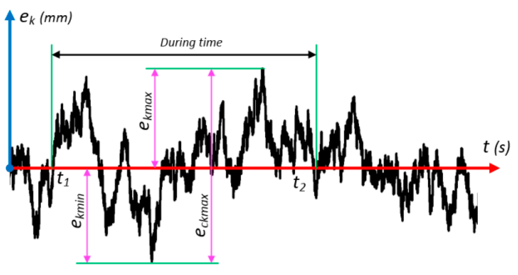
• A procedure for evaluating the tracking performance of the MMP system under disturbances and sensor faults is proposed. Based on this evaluation process, the performance level achieved during simulations and experiments can be easily obtained.
• Our major contribution in this paper shows that the proposed SFTC technique is successfully applied to reduce minimum impacts of faults and disturbances aimed at stability and safety insurance for the system.

This paper is organized as follows. In Section 2, the mathematical model of the MMP EHA system with disturbances and sensor faults is presented. In Section 3, a UIO reconstruction formulated for the nonlinear discrete-time system is performed to satisfy the discrete-time Lipschitz condition and ensure asymptotic stability of the state observer under the LMI optimization algorithm. In Section 4, an SFTC technique is proposed for the fault compensation process based on the sensor fault estimation and the residual signals. In Section 5, numerical simulations and experimental results are presented, and these results are evaluated. Section 6 contains a discussion of the results. Finally, conclusions are presented in Section 7.

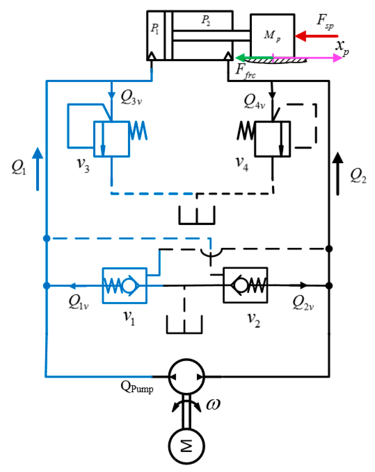
2. Modeling of the EHA System

Considering the dynamics equations of the MMP EHA system, the model in Figure 1 can be derived using Newton’s Second Law to describe the object M_p [3]:

$$m_p{\ddot{x}}_p+B_v{\dot{x}}_p+F_{sp}+F_{frc}+d=A_1{P}_1-A_2{P}_2$$

(1)

Here, $m_p$ is the equivalent mass, while $x_p$, ${\dot{x}}_p$, and ${\ddot{x}}_p$ are the position, velocity, and acceleration, respectively; $A_1$ and $A_2$ are the area in the two chambers; $F_{sp}$, $F_{frc}$, $B_v$, and d are the external load force of the spring, friction force, viscous damping coefficient, and bounded UID, respectively; and $P_1$ and $P_2$ are the pressures in the two chambers.

The spring force $F_{sp}$ can be represented as

$$F_{sp}=K_{sp}{x}_p,$$

(2)

where $K_{sp}$ is the spring stiffness.

The $F_{frc}$ friction force can be represented as [29]

$$F_{frc}=\sqrt{2e}\left(F_{brk}-F_C\right)e^{-{\left(\frac{v_p}{v_{st}}\right)}^2}\hspace{0.17em}\frac{v_p}{v_{st}}\hspace{0.17em}\hspace{0.17em}+F_C\hspace{0.17em}\tanh \left(\frac{v_p}{v_{st}}\right)\hspace{0.17em}\hspace{0.17em},$$

(3)

where $F_{brk}$ and $F_C$ are the breakaway friction and the Coulomb friction, respectively; and $v_p$ and $v_{st}$ are the velocity and Stribek velocity threshold, respectively.

The hydraulic continuity equations for the EHA system can be described as [3]

$${\dot{P}}_1={\Delta }_1\left(Q_1-Q_i-A_1{\dot{x}}_p\right),$$

(4)

$${\dot{P}}_2={\Delta }_2\left(Q_2+Q_i+A_2{\dot{x}}_p\right),$$

(5)

where

$${\Delta }_1={\beta }_e/\left(V_{01}+A_1{x}_p\right),\hspace{0.17em}{\Delta }_2={\beta }_e/\left(V_{02}-A_2{x}_p\right),Q_{13i}=Q_{1v}-Q_{3v}-Q_i,\mathrm{and}{Q}_{24i}=Q_{2v}-Q_{4v}+Q_i.$$

${\beta }_e$ and $Q_i$ are the effective bulk modulus in each chamber and the internal leakage flow rate of the cylinder, respectively; and $V_{01}$ and $V_{02}$ are the initial control volumes of the first and the second chamber, respectively [3].

$$\begin{array}{l}{Q}_1=Q_{pump}+Q_{1v}-Q_{3v}\\ Q_2=-Q_{pump}+Q_{2v}-Q_{4v}\end{array}$$

(6)

Here, $Q_{pump}=D_p\omega$. $Q_{1v}$ and $Q_{2v}$ are the flow rate through the pilot-operated check valve on the left and on the right, respectively. $Q_{3v}$, $Q_{4v}$ and $Q_{pump}$ are the flow rates through the pressure relief valve on the left, on the right, and the pump flow rate, respectively. $D_p$ and $\omega$ are the displacement and the speed of the servo pump, as shown in Figure 1.

Based on the system’s dynamics equations shown in Equations (1)–(6), the dynamic equation for the system can be represented by a state vector ${\left[\begin{array}{cccc}{x}_1& x_2& x_3& x_4\hspace{0.17em}\end{array}\right]}^T={\left[\begin{array}{cccc}{x}_p& {\dot{x}}_p& P_1& P_2\hspace{0.17em}\end{array}\right]}^T$ and rewritten as

$$\left[\begin{array}{c}{\dot{x}}_1\\ {\dot{x}}_2\\ {\dot{x}}_3\\ {\dot{x}}_4\end{array}\right]=\left[\begin{array}{c}{x}_2\\ \frac{1}{m_p}\left[\left(A_1{x}_3-A_2{x}_4\right)-B_v-F_{frc}-K_{sp}{x}_1-d\right]\\ \frac{{\beta }_e}{V_{01}+A_1{x}_1}\left(Q_{pump}+Q_{13i}-A_1{x}_2\right)\\ \frac{{\beta }_e}{V_{02}-A_2{x}_1}\left(-Q_{pump}+Q_{24i}+A_2{x}_2\right)\end{array}\right],$$

(7)

The system of equations expressed in (7) can be represented as

$$\dot{x}=Ax+f\left(x,u\right)+D_{d}d,$$

(8)

where

$$A=\left[\begin{array}{cccc}0& 1& 0& 0\\ {\alpha }_1& {\alpha }_2& {\alpha }_3& {\alpha }_4\\ 0& 0& 0& 0\\ 0& 0& 0& 0\end{array}\right];f\left(x,u\right)=\left[\begin{array}{c}0\\ \frac{-F_{frc}}{m_p}\\ {\Delta }_1\left(D_{p}u+Q_{13i}-A_1{x}_2\right)\\ {\Delta }_2\left(-D_{p}u+Q_{24i}+A_2{x}_2\right)\end{array}\right];D_d=\left[\begin{array}{c}0\\ \frac{-1}{m_p}\\ 0\\ 0\end{array}\right],$$

$${\alpha }_1=\frac{-K_{sp}}{m_p};{\alpha }_2=\frac{-B_v}{m_p};{\alpha }_3=\frac{A_1}{m_p};{\alpha }_4=\frac{-A_2}{m_p};u=\omega$$

Equation (8) shows that the matrix A is a constant matrix. The system of equations shown above can be rewritten as a nonlinear discrete-time state space model as shown below:

$$x_{k+1}=A_k{x}_k+{\varphi }_{x_k,u_k}+D_d{d}_k,$$

(9)

where

$$x_k={\left[\begin{array}{ccc}{x}_{1k}^T& x_{2k}^T& x_{3k}^T\hspace{0.17em}\hspace{0.17em}\hspace{0.17em}\hspace{0.17em}{x}_{4k}^T\end{array}\right]}^T,$$

$$A_k=\left[\begin{array}{cccc}1& T_s& 0& 0\\ T_s{\alpha }_1& 1+T_s{\alpha }_2& T_s{\alpha }_3& T_s{\alpha }_4\\ 0& 0& 1& 0\\ 0& 0& 0& 1\end{array}\right];{\varphi }_{x_k,u_k}=T_{s}f\left(x_k,u_k\right);\hspace{0.17em}\hspace{0.17em}{d}_k=T_{s}d$$

$T_s$ is a sampling time

Obviously, system states are performed from changing the speed of the bi-directional pump, which is controlled by a DC motor. The system is controlled via the input speed ω of the DC motor so that the output position $x_{1k}^{}$ (or the measurement output $y_k^{}$) tracks as closely as possible to a reference position $y_{rk}^{}$. Considering the influences and reducing the impacts of sensor fault on the measurement output signal are the objective of this paper, and these will be described in the following section.

3. UIO for a Nonlinear Discrete-Time System

A nonlinear discrete-time system subjected to an unknown input disturbance can be represented as follows:

$$\{\begin{array}{l}{x}_{k+1}=A_k{x}_k+B_k{u}_k\hspace{0.17em}\hspace{0.17em}+{\varphi }_{x_k,u_k}+D_d{d}_k\\ \hspace{0.17em}y{\hspace{0.17em}}_k\hspace{0.17em}=C_k{x}_k+F_s{s}_k\end{array},$$

(10)

where $x_k\in {ℝ}^n$ is the state vector, $y_k\in {ℝ}^p$ is the output vector, $d_k\in {ℝ}^r$ is the unknown input or disturbance vector, and $s_k\in {ℝ}^q$ is the sensor fault vector.$A_k,B_k,C_k,D_d$, and $F_s$ are known constant matrices with suitable dimensions. ${\varphi }_{x_k,u_k} = \varphi \left(x_k,u_k\right)$ is a nonlinear function vector $\forall x_k,x_k\in {ℝ}^n$, $u_k\in {ℝ}^m$.

If it is assumed that the Lipschitz condition applies to the discrete-time nonlinear function vector ${\varphi }_{x_k,u_k}$, then there exists a constant τ > 0 such that [8,9,11,23]

$$\Vert \Delta {\varphi }_{x_k,u_k}\Vert \le \tau \Vert x_k-{\widehat{x}}_k\Vert ,$$

(11)

where

$$\Vert \Delta {\varphi }_{x_k,u_k}\Vert =\Vert {\varphi }_{x_k,u_k}-{\varphi }_{{\widehat{x}}_k,u_k}\Vert$$

The nonlinear system (10) can be rewritten as

$$\{\begin{array}{l}\overline{E}{\overline{x}}_{k+1}={\overline{A}}_k{\overline{x}}_k\hspace{0.17em}\hspace{0.17em}+{\overline{\varphi }}_{x_k,u_k}+\overline{G}{s}_k+{\overline{D}}_d{d}_k\\ \hspace{0.17em}{y}_k\hspace{0.17em}={\overline{C}}_k{\overline{x}}_k\end{array},$$

(12)

where

$$\begin{array}{c}\hspace{0.17em}\hspace{0.17em}{\overline{A}}_k=\left[\begin{array}{cc}{A}_k& 0\\ 0& -I_p\end{array}\right];\overline{E}=\left[\begin{array}{cc}{I}_n& 0\\ 0& 0_p\end{array}\right]{\overline{D}}_d=\left[\begin{array}{c}{D}_d\\ 0\end{array}\right];{\overline{B}}_k={\left[\begin{array}{cc}{B}_k& 0\end{array}\right]}^T;\\ B_k=0;{\overline{C}}_k=\left[\begin{array}{cc}{C}_k& F_s\end{array}\right];\overline{G}={\left[\begin{array}{cc}0& I_p\end{array}\right]}^T\\ {\overline{x}}_k={\left[\begin{array}{cc}{x}_k^T& s_k{}^T\end{array}\right]}^T\in {ℝ}^{\overline{n}};\hspace{0.17em}{\overline{\varphi }}_{x_k,u_k}={\left[\begin{array}{cc}{\varphi }_{x_k,u_k}^T& 0\end{array}\right]}^T\in {ℝ}^{\overline{n}}\end{array}$$

with $\overline{n} = n + p$.

Based on [11,21], a UIO can be built for the nonlinear discrete-time system as shown below.

$$\{\begin{array}{l}{\overline{z}}_{k+1}=F{\widehat{\overline{x}}}_k+L\left(y_k-{\widehat{y}}_k\right)\hspace{0.17em}+\mathsf{\Gamma }{\overline{\varphi }}_{{\widehat{x}}_k,u_k}\\ {\widehat{\overline{x}}}_k={\overline{z}}_k+H{y}_k\\ {\widehat{y}}_k={\overline{C}}_k{\widehat{\overline{x}}}_k\end{array},$$

(13)

Here, ${\widehat{\overline{x}}}_k\in {ℝ}^{\overline{n}}$, ${\widehat{y}}_k\in {ℝ}^p$, and ${\overline{z}}_k\in {ℝ}^{\overline{n}}$ are the estimate of the state vector ${\overline{x}}_k$, the estimate of the measurement output vector, and the state vector of the observer, respectively. The observer matrices $F\in {ℝ}^{\overline{n}\times \overline{n}}$, $\mathsf{\Gamma }\in {ℝ}^{\overline{n}\times \overline{n}}$, $H\in {ℝ}^{\overline{n}\times p}$, and $L\in {ℝ}^{\overline{n}\times p}$ should be designed according to the state error vector.

The state error can be defined as

$${\overline{e}}_k={\overline{x}}_k-{\widehat{\overline{x}}}_k,$$

(14)

From Equations (12), and (13), we can write as

$$\begin{array}{ll}{\widehat{\overline{x}}}_{k+1}& =F{\widehat{\overline{x}}}_k-L{\widehat{y}}_k\hspace{0.17em}+L{y}_k+\mathsf{\Gamma }{\overline{\varphi }}_{{\widehat{x}}_k,u_k}+H{\overline{C}}_k{\overline{x}}_{k+1}\\ & =\left(F-L{\overline{C}}_k\right){\widehat{\overline{x}}}_k\hspace{0.17em}+L{y}_k+\mathsf{\Gamma }{\overline{\varphi }}_{{\widehat{x}}_k,u_k}+H{\overline{C}}_k{\overline{x}}_{k+1}\end{array}$$

(15)

Equation (12) can be written as:

$$\mathsf{\Gamma }\overline{E}{\overline{x}}_{k+1}=\mathsf{\Gamma }{\overline{A}}_k{\overline{x}}_k+\hspace{0.17em}\mathsf{\Gamma }{\overline{\varphi }}_{x_k,u_k}+\mathsf{\Gamma }\overline{G}{s}_k+\mathsf{\Gamma }{\overline{D}}_d{d}_k,$$

(16)

Subtracting (15) from (16), we obtain:

$$\begin{array}{l}\left(\mathsf{\Gamma }\overline{E}+H{\overline{C}}_k\right){\overline{x}}_{k+1}-{\widehat{\overline{x}}}_{k+1}=\left(\mathsf{\Gamma }{\overline{A}}_k-L{\overline{C}}_k\right){\overline{x}}_k\\ -\left(F-L{\overline{C}}_k\right){\widehat{\overline{x}}}_k\hspace{0.17em}\hspace{0.17em}+\hspace{0.17em}\mathsf{\Gamma }\Delta {\overline{\varphi }}_{x_k,u_k}+\mathsf{\Gamma }\overline{G}{s}_k+\mathsf{\Gamma }{\overline{D}}_d{d}_k\end{array}$$

(17)

Based on Equations (16) and (17), the estimation error of Equation (16) can be written as

$${\overline{e}}_{k+1}=N{\overline{e}}_k+\mathsf{\Gamma }\Delta {\overline{\varphi }}_{x_k,u_k}+\mathsf{\Gamma }{\overline{D}}_d{d}_k,$$

(18)

where

$$N=\mathsf{\Gamma }{\overline{A}}_k-L{\overline{C}}_k,$$

(19)

If the following conditions are satisfied:

$$\mathsf{\Gamma }\overline{E}+H{\overline{C}}_k=I_{\overline{n}},$$

(20)

$$\mathsf{\Gamma }\overline{G}=0$$

(21)

$$\mathsf{\Gamma }{\overline{A}}_k-L{\overline{C}}_k=N$$

(22)

$$\mathsf{\Gamma }{\overline{A}}_k=F$$

(23)

Without loss of generality, the matrix $\mathsf{\Gamma }$ can be defined as

$$\mathsf{\Gamma }=\left[\begin{array}{cc}{I}_n& {\varphi }_1\\ -{\overline{C}}_k& {\varphi }_2\end{array}\right],$$

(24)

where ${\varphi }_1\in {ℝ}^{nxp}$ and ${\varphi }_2\in {ℝ}^{pxp}$ are arbitrary matrices.

By solving the system in Equations (20) to (24), we obtain:

$$\mathsf{\Gamma }=\left[\begin{array}{cc}{I}_n& 0\\ -{\overline{C}}_k& 0\end{array}\right];\hspace{0.17em}{\varphi }_1={\varphi }_2=0,$$

(25)

and

$$H={\left[\begin{array}{cc}0& I_p\end{array}\right]}^T,$$

The inequality in Equation (11) needs to be satisfied for the nonlinear function $\Delta {\overline{\varphi }}_{x_k,u_k}$ as:

$$\Vert \Delta {\overline{\varphi }}_{x_k,u_k}\Vert \le \overline{\tau }\Vert {\overline{x}}_k-{\widehat{\overline{x}}}_k\Vert ,$$

(26)

where

$$\overline{\tau }=\left[\begin{array}{cc}\tau I_n& 0\\ 0& \hspace{0.17em}{0}_p\end{array}\right]\in {ℝ}^{\overline{n}}$$

From (26), the matrix $\mathsf{\Xi }$ can be written as follows:

$$\mathsf{\Xi }={\left[\begin{array}{c}{\overline{e}}_k\\ \Delta {\overline{\varphi }}_{x_k,u_k}\end{array}\right]}^T\left[\begin{array}{cc}-{\overline{\tau }}^T\overline{\tau }& 0\\ 0& I_{\overline{n}}\end{array}\right]\left[\begin{array}{c}{\overline{e}}_k\\ \Delta {\overline{\varphi }}_{x_k,u_k}\end{array}\right]\le 0,$$

(27)

Lemma 1

([9]). The necessary and sufficient conditions for the existence of the UIO in (13) for the system in (12) are as follows.

(a)

$rank(C_k{D}_d)=rank(D_d)$

(b)

$\left[\begin{array}{cc}{A}_k-I_n& D_d\\ C_k& 0\end{array}\right]=n+p$, and$D_d$is a full column rank

(c)

$\left[\begin{array}{cc}{A}_k-z{I}_n& D_d\\ C_k& 0\end{array}\right]=n+p\hspace{0.17em}\hspace{0.17em}\hspace{0.17em}\hspace{0.17em}\forall z$with$\left|z\right|>1$

Lemma 2

([12]). For the following equation

$${\zeta }_{k+1}=\mathsf{\Phi }{\zeta }_k+\Upsilon u_k,$$

(28)

the eigenvalues of the matrix $\mathsf{\Phi }\in {ℝ}^{n\times n}$ belong to the circular region $D\left(\alpha ,\rho \right)$ with center α + j0 and radius $\rho$ if and only if there exists a symmetric positive definite matrix $P\in {ℝ}^{n\times n}$ such that the following condition hold

$$\left[\begin{array}{cc}-P& P\left(\mathsf{\Phi }-\alpha I_n\right)\\ \ast & -{\rho }^{2}P\end{array}\right]<0,$$

(29)

Theorem 1.

For system (12), there exists a robust UIO in the form of (13) such that the output error satisfies$\Vert e_{yk}\Vert \le \mu \Vert d_k^{}\Vert$in a prescribed circular region$D\left(\alpha ,r\right)$if there exists a positive-definite symmetric matrix$\overline{P}\in {ℝ}^{\overline{n}\times \overline{n}}$, matrix$\overline{Q}\in {ℝ}^{\overline{n}\times p}$, and positive scalars$\mu ,$and$\epsilon$such that the following inequalities hold:

$$\left[\begin{array}{ccccc}-\mu I_p& 0& {\overline{C}}_k& 0& 0\\ \ast & -\overline{P}& \overline{P}\mathsf{\Gamma }{\overline{A}}_k^{}-\overline{Q}{\overline{C}}_k^{}& \overline{P}\mathsf{\Gamma }& \overline{P}\left(\mathsf{\Gamma }{\overline{D}}_d\right)\\ \ast & \ast & -\overline{P}+\epsilon {\overline{\tau }}_{}^T\overline{\tau }& 0& 0\\ \ast & \ast & \ast & -\epsilon I_{\overline{n}}& 0\\ \ast & \ast & \ast & \ast & -\mu I_d\end{array}\right]<0,$$

(30)

and

$$\left[\begin{array}{cc}-\overline{P}& \overline{P}\mathsf{\Gamma }{\overline{A}}_k-\overline{Q}{\overline{C}}_k-\alpha \overline{P}\\ \ast & -r^2\overline{P}\end{array}\right]<0,$$

(31)

where$\overline{Q} = \overline{P}L$.

Then, the state observer (13) is asymptotically stable.

Proof of Equation (26).

Consider a Lyapunov function $V_k = {\overline{e}}_k^T\overline{P}{\overline{e}}_k$. The difference between two adjacent steps of the Lyapunov function $\Delta V_k = V_{k+1}-V_k$ is calculated as

$$\begin{array}{ll}\Delta V_k& =V_{k+1}-V_k\\ & ={\overline{e}}_{k+1}^T\overline{P}{\overline{e}}_{k+1}-{\overline{e}}_k^T\overline{P}{\overline{e}}_k\\ & ={\lambda }^T\left[\begin{array}{ccc}{N}_{}^T\overline{P}N-\overline{P}& N_{}^T\overline{P}\mathsf{\Gamma }& N_{}^T\overline{P}\mathsf{\Gamma }{\overline{D}}_d\\ \ast & {\mathsf{\Gamma }}^T\overline{P}\mathsf{\Gamma }& {\mathsf{\Gamma }}^T\overline{P}\mathsf{\Gamma }{\overline{D}}_d\\ \ast & \ast & {\left(\mathsf{\Gamma }{\overline{D}}_d\right)}^T\overline{P}\mathsf{\Gamma }{\overline{D}}_d\end{array}\right]\lambda \end{array}$$

(32)

where $\lambda = {\left[\begin{array}{ccc}{\overline{e}}_k^T& \Delta {\overline{\varphi }}_{x_k,u_k}^T& d_k^T\end{array}\right]}^T$.

Moreover, Equation (27) can be expressed as:

$$\mathsf{\Xi }={\lambda }^T\left[\begin{array}{ccc}-{\overline{\tau }}^T\overline{\tau }& 0& 0\\ 0& I_{\overline{n}}& 0\\ 0& 0& 0\end{array}\right]\lambda \le 0,$$

(33)

Combining Equations (32) and (33) leads to:

$$\begin{array}{ll}\Delta V_k& \le {\lambda }^T\left[\begin{array}{ccc}{N}_{}^T\overline{P}N-\overline{P}& N_{}^T\overline{P}\mathsf{\Gamma }& N_{}^T\overline{P}\mathsf{\Gamma }{\overline{D}}_d\\ \ast & {\mathsf{\Gamma }}^T\overline{P}\mathsf{\Gamma }& {\mathsf{\Gamma }}^T\overline{P}\mathsf{\Gamma }{\overline{D}}_d\\ \ast & \ast & {\sigma }_{33}\end{array}\right]\lambda -\epsilon \mathsf{\Xi }\\ & ={\lambda }^T\left[\begin{array}{ccc}{\sigma }_{11}& N_{}^T\overline{P}\mathsf{\Gamma }& N_{}^T\overline{P}\mathsf{\Gamma }{\overline{D}}_d\\ \ast & {\sigma }_{22}& {\mathsf{\Gamma }}^T\overline{P}\mathsf{\Gamma }{\overline{D}}_d\\ \ast & \ast & {\sigma }_{33}\end{array}\right]\lambda \end{array}$$

(34)

where

$$\begin{array}{l}{\sigma }_{11}=N_{}^T\overline{P}N-\overline{P}+\epsilon {\overline{\tau }}^T\overline{\tau };\hspace{0.17em}{\sigma }_{33}={\left(\mathsf{\Gamma }{\overline{D}}_d\right)}^T\overline{P}\mathsf{\Gamma }{\overline{D}}_d\\ {\sigma }_{22}={\mathsf{\Gamma }}^T\overline{P}\mathsf{\Gamma }-\epsilon I_{\overline{n}}\end{array}$$

To satisfy the measurement error condition $\Vert e_{yk}\Vert \le \mu \Vert d_k\Vert$ of the output, the matrix $\mathsf{\Theta }$ can be represented as

$$\mathsf{\Theta }={\left[\begin{array}{c}{\overline{e}}_k\\ d_k\end{array}\right]}^T\left[\begin{array}{cc}\frac{1}{\mu }{\overline{C}}_k^T{\overline{C}}_k& 0\\ 0& -\mu I_d\end{array}\right]\left[\begin{array}{c}{\overline{e}}_k\\ d_k\end{array}\right]\le 0,$$

(35)

Using Equations (32) and (35), the matrix $T_n$ can be written as

$$T_n=\Delta V_k+\mathsf{\Theta }\le 0,$$

(36)

Finally, an inequality of matrix $T_n$ can be represented as

$$\begin{array}{ll}{T}_n& \le {\lambda }^T\left[\begin{array}{ccc}{\sigma }_{11}+\frac{1}{\mu }{\overline{C}}_k^T{\overline{C}}_k& N_{}^T\overline{P}\mathsf{\Gamma }& N_{}^T\overline{P}\mathsf{\Gamma }{\overline{D}}_d\\ \ast & {\sigma }_{22}& {\mathsf{\Gamma }}^T\overline{P}\mathsf{\Gamma }{\overline{D}}_d\\ \ast & \ast & {\sigma }_{33}-\mu I_d\end{array}\right]\lambda \\ & ={\lambda }^T{\mathsf{\Pi }}_n\lambda \end{array}$$

(37)

where

$$\begin{array}{ll}{\mathsf{\Pi }}_n& =\left[\begin{array}{ccc}-\overline{P}+\epsilon {\overline{\tau }}^T\overline{\tau }+\frac{1}{\mu }{\overline{C}}_k^T{\overline{C}}_k& 0& 0\\ \ast & -\epsilon I_{\overline{n}}& 0\\ \ast & \ast & -\mu I_d\end{array}\right]\hspace{0.17em}\\ & +\left[\begin{array}{ccc}{N}^T\overline{P}N& N^T\overline{P}\mathsf{\Gamma }& N^T\overline{P}\mathsf{\Gamma }{\overline{D}}_d\\ \ast & {\mathsf{\Gamma }}^T\overline{P}\mathsf{\Gamma }& {\mathsf{\Gamma }}^T\overline{P}\mathsf{\Gamma }{\overline{D}}_d\\ \ast & \ast & {\left(\mathsf{\Gamma }{\overline{D}}_d\right)}^T\overline{P}\mathsf{\Gamma }{\overline{D}}_d\end{array}\right]\end{array}$$

(38)

Applying the Schur Complement Lemma [33] to Equation (38) for ${\mathsf{\Pi }}_n < 0$, we have:

$${\mathsf{\Pi }}_{n{}^{\prime }}=\left[\begin{array}{cccc}-\overline{P}& \overline{P}\mathsf{\Gamma }{\overline{A}}_k-\overline{P}L{\overline{C}}_k^{}& \overline{P}\mathsf{\Gamma }& \overline{P}\mathsf{\Gamma }{\overline{D}}_d\\ \ast & -\overline{P}+\epsilon {\overline{\tau }}_{}^T\overline{\tau }+\frac{1}{\mu }{\overline{C}}_k^T{\overline{C}}_k& 0& 0\\ \ast & \ast & -\epsilon I_{\overline{n}}& 0\\ \ast & \ast & \ast & -\mu I_d\end{array}\right],$$

(39)

Similarly, Equation (30) is satisfied by applying the Schur Complement Lemma [32] to Equation (39) for ${\mathsf{\Pi }}_{n{}^{\prime }} < 0$. □

Proof of Equation (27).

Using Lemma 2, inequality (31) is met by applying Equation (18). □

In summary, the design procedure for the sensor fault estimator consists of the following steps:

Step 1:

Build the augmented system (12) for the nonlinear discrete-time system (10).

Step 2:

Determine the matrices $\overline{Q}$, $\overline{P}$, $F$, and $L = {\overline{P}}_{}^{-1}\overline{Q}$ by solving the LMI matrix inequalities (30) and (31).

Step 3:

Obtain the state estimate and the fault estimate as ${\widehat{x}}_k^{} = \left[\begin{array}{cc}{I}_n& o_{n\times p}\end{array}\right]{\widehat{\overline{x}}}_k^{}$, and ${\widehat{s}}_k = {\overline{C}}_s{\widehat{\overline{x}}}_k$, respectively, where ${\overline{C}}_s=\left[\begin{array}{cc}{o}_{r\times n}& I_p\end{array}\right]$.

Remark 1.

This UIO reconstruction only applies to observable systems. For systems that are not possible to observe, the reduced-order observer construction shown in [33,34] should be applied.

Remark 2.

This paper uses the sensor fault reconstruction in [8,26] to design a discrete-time nonlinear observer system for the state observer that is asymptotically stable. Here, constructing and proving Theorem 1 to apply the LMI optimization algorithm was made simpler [8] by using Lyapunov’s stability under matrix equations. With this sensor fault reconstruction, it is possible to estimate the faults using the UIO model, which has advantages such as directly estimating the sensor fault on the UIO without decoupling the disturbance matrix, as shown in [9].

Remark 3.

Constructing a robust UIO reconstruction method using LMI optimization algorithm was utilized by a function$H_{\infty }$as performed in [8]. However, in this paper, by applying Lyapunov stability theory under the formulated matrix equations, a robust UIO reconstruction method for using the LMI optimization algorithm was demonstrated that was simpler than in [8], and in which the state observer is asymptotically stable.

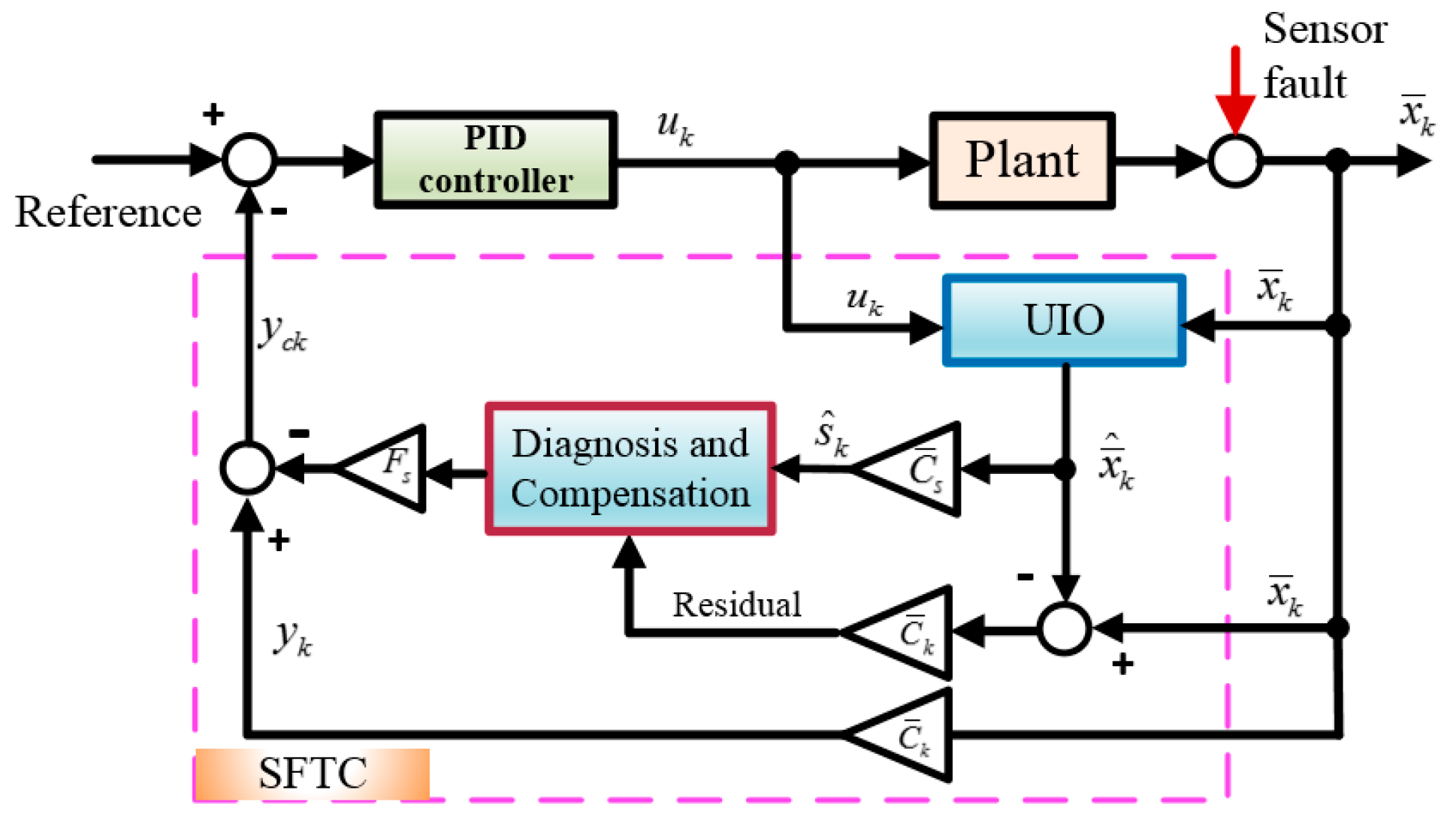
4. Sensor Fault-Tolerant Control for the MMP System

4.1. Fault Diagnosis-Based General Residual from the Sensor Fault Signal

The general residual due to a sensor fault is defined as the difference between the response signal and the feedback estimation signal from the UIO. The residual vector is calculated as [11]

$$r_k=y_k-{\widehat{y}}_k,$$

(40)

The FD method consists of two main tasks: fault detection and fault isolation. The fault detection process involves determining whether a fault has occurred based on information from the RS, which means that $r_k = 0$ if $s_k=0$ without fault, and $r_k \ne 0$ if $s_k \ne 0$ with fault [11]. The fault isolation process is executed to make a binary decision signal based on the fault detection process through executing logic that is constructed via the RS and the threshold value k. The binary decision signal is 0 when $\left|r_k\right| \le k$, and conversely, this signal is 1 when $\left|r_k\right| > k$.

4.2. Sensor FTC Compensation

Sensor fault output from the measurements influences the closed-loop behavior and corrupts the state estimation.

The FTC designed to diagnose the position SFs of the MMP system is shown in Figure 2. The PID main controller performs conventional closed-loop position tracking control such that the measurement signal is employed, as in [5]

$$y_{ck}=y_k-F_s{\widehat{s}}_k,$$

(41)

Fault compensation is performed by a logical process wherein fault magnitude is received from the estimated fault signal based on the residual signal to make a control decision based on the binary signal. The fault compensation process will not be executed if the binary decision signal has a value equal to 0; otherwise, if the binary decision signal is equal to 1, the fault compensation process will be executed using the threshold k. [11].

4.3. PID Control for MMP System

The control error is one of the most important factors to be chosen for evaluating the PID controller performance. The control error is defined as

$$e_k=y_r-y_{ck},$$

(42)

The maximum position error $e_{k\max }$ of the position control error $e_k$ shown in Figure 3 can be described as

$$e_{k\max }=y_{r\max }-y_{ck\max },$$

(43)

where $y_{r\max }$ and $y_{ck\max }$ are the maximum values of the reference and response signals in the time period (t₁, t₂).

The minimum position error $e_{k\min }$ of the position control error $e_k$ is computed for the time period (t₁, t₂) in Figure 3 as

$$e_{k\min }=y_{r\min }-y_{ck\min },$$

(44)

where t₁ and t₂ are the begin time and the end time of the time period used to calculate the position control error. During the time period (t₁, t₂), $y_{r\min }$ and $y_{ck\min }$ are the minimum reference signal and the minimum response signal, respectively, as shown in Figure 3.

The maximum control error of the system during the time (t₁, t₂) is obtained as

$$e_{ck\max }=\max \left(\left|e_{k\max }\right|,\left|e_{k\min }\right|\right),$$

(45)

The control error performance ${\eta }_k$ of the system is defined as follows based on the maximum control error $e_{ck\max }$ during the time period (t₁, t₂):

$${\eta }_k=\left(1-\frac{e_{ck\max }}{s_{k\max }}\right)\times 100\hspace{0.17em}(\%),$$

(46)

$$s_{k\max }=s_{\max }-s_{\min }$$

(47)

where $s_{\max }$ and $s_{\min }$ are the maximum and minimum sensor faults, respectively, during the time period (t₁, t₂).

To explicitly evaluate the effect of a fault, the sensor fault error $e_{sfk}$ is defined as

$$e_{sfk}=e_{fk}-e_{0ck},$$

(48)

where $e_{fk}$ and $e_{0ck}$ are the position control error in the case of sensor fault and the position control error for the case without sensor fault, respectively.

The maximum sensor fault error $e_{sfk\max }$ of the sensor fault error $e_{sfk}$ is computed as

$$e_{sfk\max }=\max \left(\left|e_{fk\max }\right|,\left|e_{0ck\max }\right|\right),$$

(49)

Similarly, the control error performance ${\xi }_k$ of the system during the time period (t₁, t₂) is calculated in terms of the sensor fault error $e_{sfk\max }$ as

$${\xi }_k=\left(1-\frac{e_{sfk\max }}{s_{k\max }}\right)\times 100\hspace{0.17em}(\%),$$

(50)

5. Simulation and Experiment Results

5.1. Parameters of the MMP System

Determining the parameters of the MMP system is complex and difficult when the parameters of the theory system are similar to the parameters of the experimental system. Therefore, we determined the main parameters of the MMP real system to specify the parameters of the real system. These parameters are defined as shown in

Table 1. Basic parameters of the MMP system.

Components	Values	Units
Ah	0.0013	m2
Ar	9.4 × 10-4	m2
Vch	2.09 × 10-4	m3
Vcr	4.0065 × 10-5	m3
mp	10	kg
${\beta }_e$	2.9 × 108	Pa
$K_{sp}$	2383	Nm
ρ	870	Kg/m3
Dp	2.5 × 10−6	m3

based on the values of a real system, namely, a KYB MMP with a φ40–φ20–250 mm cylinder and a 24V DC motor. After the fundamental parameters were confirmed by normal calculations, the other parameters were determined by using the parameter estimation method in Matlab. Finally, the main parameters of the MMP real system are listed in Table 1.

The parameters of the MMP model in Equation (9) were determined to be

$$B_k=\left[\begin{array}{ccc}0& 0& 0\hspace{0.17em}\hspace{0.17em}\hspace{0.17em}\hspace{0.17em}0\end{array}\right]{\hspace{0.17em}}^T;C_k=\left[\begin{array}{ccc}1& 0& 0\hspace{0.17em}\hspace{0.17em}\hspace{0.17em}\hspace{0.17em}0\end{array}\right];F_s=1;T_s=0.001\hspace{0.17em}$$

$$A_k=\hspace{0.17em}\left[\begin{array}{cccc}1& T_s& 0& 0\\ -1.8311\mathrm{e}-01& 9.4639\mathrm{e}-01& 9.7297\mathrm{e}-08& -9.1700\mathrm{e}-08\\ 0& 0& 1& 0\\ 0& 0& 0& 1\end{array}\right]$$

where a sampling time $T_s = 0.001\left(s\right)$ is applied to all of the simulation processes.

The reference signal is given as

$$y_r\left(t\right)=1.5\sin (0.8t)+1.5,$$

(51)

We assume that the sensor fault $s(t)$ is given as

$$s(t)=\{\begin{array}{ll}0& \mathrm{if}\hspace{0.17em}\hspace{0.17em}t<11\\ 1.5t-16.5& \mathrm{if}\hspace{0.17em}\hspace{0.17em}11\hspace{0.17em}\le t\le 12\\ 2251.5-187.5t& \mathrm{if}\hspace{0.17em}\hspace{0.17em}12\le t\le 12.008\\ 0& \mathrm{if}\hspace{0.17em}\hspace{0.17em}12.5\hspace{0.17em}\hspace{0.17em}\le t\le 22.75\\ 5t-455/4& \mathrm{if}\hspace{0.17em}\hspace{0.17em}\hspace{0.17em}22.75\hspace{0.17em}\le t\le 23\\ 1.25& \mathrm{if}\hspace{0.17em}\hspace{0.17em}\hspace{0.17em}23\le t\le 29.5\\ 150-5t& \mathrm{if}29.5\le t\le 30\\ 0& \mathrm{if}\hspace{0.17em}\hspace{0.17em}t>30\end{array},$$

(52)

Based on design experience, we chose positive scalars $\tau = 30$, $r = 0.05$, $\alpha = 0.3$, $\epsilon = 0.2$, and $\mu = 0.1$. We can solve for the matrices $\overline{P}$, $\overline{Q}$, $L$ and $F$ using the LMI defined in (30), and (31) if the solution is feasible. We obtained the following results:

$$\mathsf{\Gamma }=\left[\begin{array}{ccccc}1& 0& 0& 0& 0\\ 0& 1& 0& 0& 0\\ 0& 0& 1& 0& 0\\ 0& 0& 0& 1& 0\\ -1& 0& 0& 0& 0\end{array}\right],H=\left[\begin{array}{c}0\\ 0\\ 0\\ 0\\ 1\end{array}\right]\overline{Q}=\hspace{0.17em}\left[\begin{array}{l}-3.5384\mathrm{e}+01\\ 1.6396\mathrm{e}-05\\ -5.8678\mathrm{e}-12\\ 5.5310\mathrm{e}-12\\ -3.5384\mathrm{e}+01\end{array}\right];L=\left[\begin{array}{l}6.0184\mathrm{e}+03\\ -1.4685\mathrm{e}+02\\ -2.0567\mathrm{e}-04\\ 1.9385\mathrm{e}-04\\ -6.0187\mathrm{e}+03\end{array}\right]$$

$$\overline{P}=[\begin{array}{ccc}1.1636\mathrm{e}+02& -6.0117\mathrm{e}-05& 1.8585\mathrm{e}-11\\ -6.0117\mathrm{e}-05& 3.5111\mathrm{e}-09& -1.5609\mathrm{e}-16\\ 1.8585\mathrm{e}-11& -1.5609\mathrm{e}-16& 3.3143\mathrm{e}-09\\ -1.7518\mathrm{e}-11& 1.4711\mathrm{e}-16& -1.4222\mathrm{e}-23\\ 1.1636\mathrm{e}+02& -6.0116\mathrm{e}-05& 1.8585\mathrm{e}-11\end{array}\begin{array}{cc}-1.7518\mathrm{e}-11& 1.1636\mathrm{e}+02\\ 1.4711\mathrm{e}-16& -6.0116\mathrm{e}-05\\ -1.4222\mathrm{e}-23& 1.8585\mathrm{e}-11\\ 3.3143\mathrm{e}-09& -1.7518\mathrm{e}-11\\ -1.7518\mathrm{e}-11& 1.1636\mathrm{e}+02\end{array}]$$

$$F=[\begin{array}{ccc}9.9991\mathrm{e}-01& 9.7297\mathrm{e}-04& 4.9095\mathrm{e}-11\\ -1.8311\mathrm{e}-01& 9.4639\mathrm{e}-01& 9.7297\mathrm{e}-08\\ 0& 0& 1\\ 0& 0& 0\\ -9.9991\mathrm{e}-01& -9.7297\mathrm{e}-04& -4.9095\mathrm{e}-11\end{array}\begin{array}{cc}-4.6271\mathrm{e}-11& 0\\ -9.1700\mathrm{e}-08& 0\\ 0& 0\\ 1& 0\\ 4.6271\mathrm{e}-11& 0\end{array}]$$

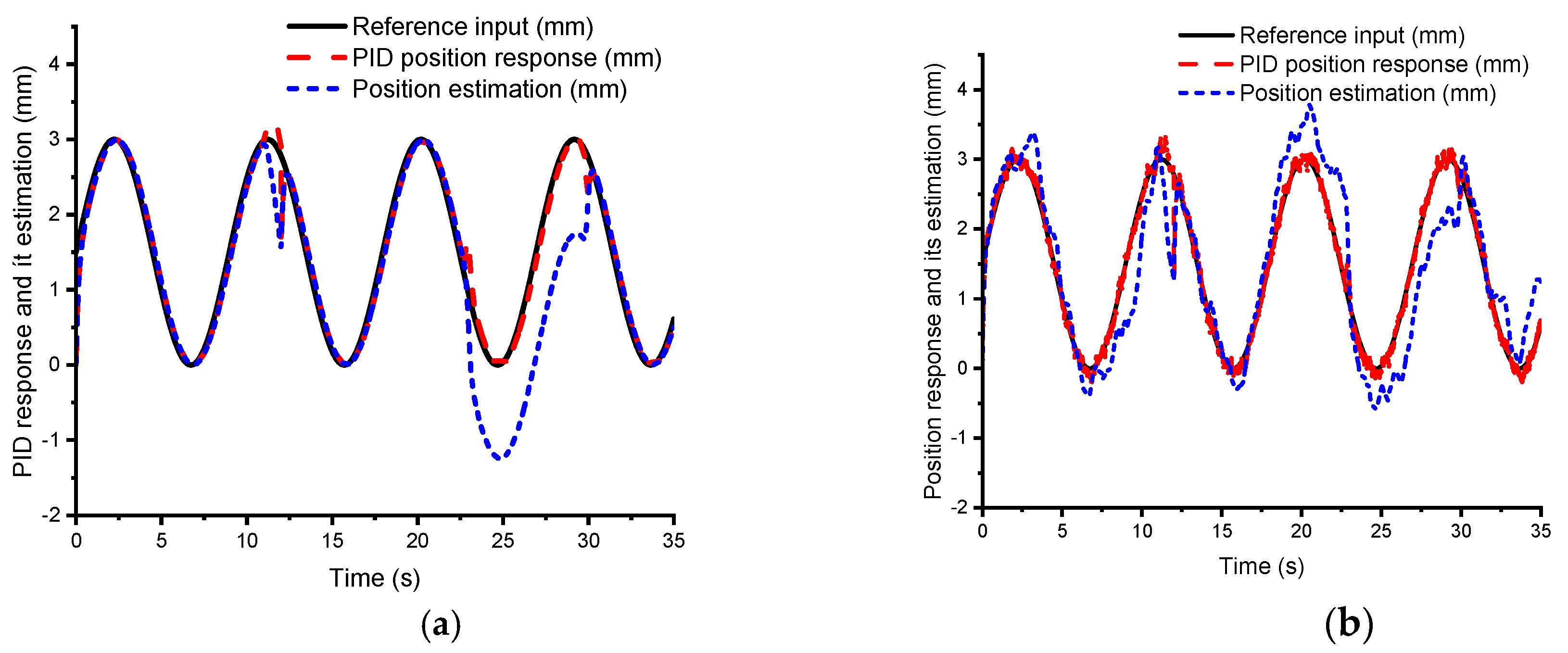
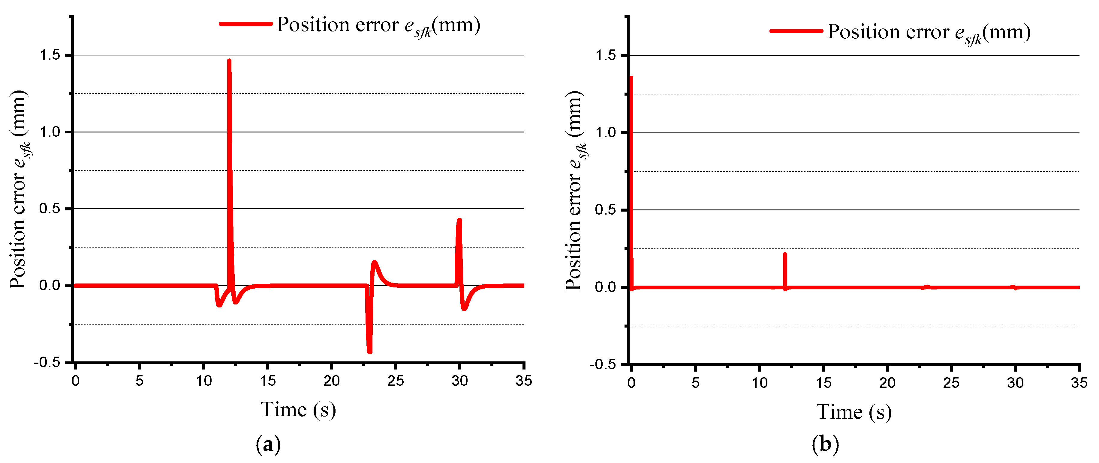
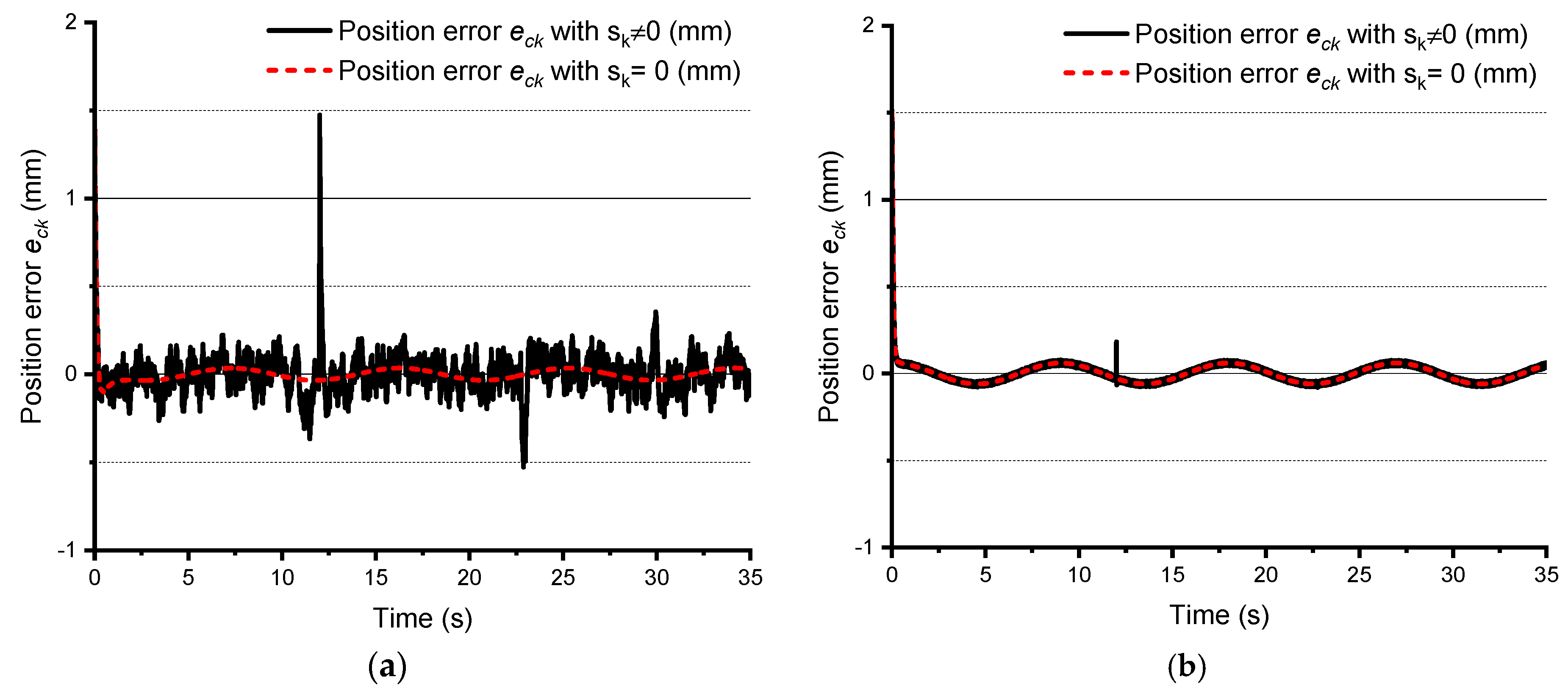
5.2. Simulation Results

A model of the sensor FTC for the MMP system was constructed in Simulink to perform numerical simulations using input and output signals where we assumed that the sensor is faulty, as described by Equation (52). Simulation results of the MMP system were compared between a system without UID ($d_k = 0$) and a system with UID $d_k = 0.0025rand(2,t)\hspace{0.17em}$(mm), which are shown in Figures 5–8. Here, the PID controller parameters (K_P = 1.63193, K_I= 2.45106, and K_D= 0.01068) are used in all simulations with a set point of the initial state in the system $x_{0k} = {\left[0,0,0\right]}^T$.

The simulation results in Figure 4a show the effects of the fault on the PID position response signal, as well as the fault estimate from 11s to 12.008 s, and from 22.75 s to 30 s for the case without FTC. We can also see that the PID position response signal follows the reference signal at locations where there is no fault impact.

In contrast, the PID position response signal does not follow the reference signal at locations where there is a fault change. The PID position response signal shown in Figure 4b is also affected by an unknown disturbance of the actuator. Additionally, the sensor fault and its estimate are similar to one another, as shown in Figure 5a, which means that the fault estimator of the UIO works well. A big difference between the sensor fault and the estimated fault is observed in Figure 5b under the impact of the disturbance $d_k$.

In contrast, we see in Figure 6a,b that the PID position response signal and the reference signal are approximately the same when the SFTC technique is applied to implement the fault compensation process. The system still operates normally, even when the fault and disturbance are compounded. Figure 6 shows that the response signal nearly replicates the desired signal, and this issue also proves that the PID position response signal with the disturbance and without disturbance is approximately the same, although the system is impacted by the disturbance.

The simulation results in Figure 7a,b shows that the sensor fault and disturbance of the actuator decreased to approximately zero after the SFTC compensation procedure. This demonstrates that the SFTC technique and the sensor fault estimator work well for the MMP system. Disturbances coming from the actuator can be cancelled after each fault compensation, so we can use only a sensor FTC for fault compensation without needing an additional actuator FTC for fault compensation.

The results of the PID controller performance are shown in

Table 2. Error assessment $e_{ck\max }$ using the PID controller.

Content	Without FTC				With FTC
	${\mathit{d}}_{\mathit{k}}=0$		$\mathbf{With}{\mathit{d}}_{\mathit{k}}$		${\mathit{d}}_{\mathit{k}}=0$		$\mathbf{With}{\mathit{d}}_{\mathit{k}}$
	${\mathit{e}}_{\mathit{c}\mathit{k}\mathbf{max}}\left(\mathit{mm}\right)$	${\mathit{\eta }}_{\mathit{k}}(\%)$	${\mathit{e}}_{\mathit{c}\mathit{k}\mathbf{max}}\left(\mathit{mm}\right)$	${\mathit{\eta }}_{\mathit{k}}(\%)$	${\mathit{e}}_{\mathit{c}\mathit{k}\mathbf{max}}\left(\mathit{mm}\right)$	${\mathit{\eta }}_{\mathit{k}}(\%)$	${\mathit{e}}_{\mathit{c}\mathit{k}\mathbf{max}}\left(\mathit{mm}\right)$	${\mathit{\eta }}_{\mathit{k}}(\%)$
From 0.1 s to 15 s	1.424	5.06	1.450	3.30	0.175	88.33	0.185	87.65
From 15 s to 25 s	0.431	65.53	0.608	51.40	0.041	96.71	0.062	95.07
From 25 s to 35 s	0.388	68.97	0.480	61.57	0.139	92.98	0.062	95.03
Average error performance $e_{ck\max }$ from 0.1s to 35s	-	46.52	-	38.77	-	92.67	-	92.58

. The results were used to evaluate the effectiveness of the SFTC technique of the PID controller based on data related to the maximum control error $e_{ck\max }$ and the control error performance ${\eta }_k$. The evaluation was conducted by numerical simulation with and without a disturbance and corresponding cases with SFTC and without SFTC, respectively. We can clearly see that the maximum control error $e_{ck\max }$ for the case without a disturbance strongly decreased when SFTC was applied, which decreased from 1.424 to 0.175 from 0.1 s to 15 s, 0.431 to 0.041 during 15 s to 25 s, and 0.388 to 0.139 from 25 s to 35 s. The control error performance ${\eta }_k$ of the PID controller was high when the SFTC was used, as it showed the average error performance $e_{ck\max }$ (${\eta }_k$) increased from 46.52% to 92.67% for the cases without and with SFTC, respectively. Similar results also show the maximum control error $e_{ck\max }$ for the cases when the disturbance strongly dropped from 1.450 to 0.185, 0.608 to 0.062, and 0.480 to 0.062, corresponding to times of 0.1 s to 15 s, 15 s to 25 s, and 25 s to 35 s, respectively, while the average error performance $e_{ck\max }$ (${\eta }_k$) significantly increased from 38.77% to 92.58% when SFTC was employed, as shown in Table 2. The disturbance showed a pretty big influence in the case without SFTC, with an average error performance $e_{ck\max }$ from 46.52% to 38.77% which is compared to average error performances $e_{ck\max }$ from 92.67% to 92.58% for the case using SFTC. Overall, most of the impacts of the disturbance and sensor fault were reduced under SFTC technology.

Moreover, the results in Figure 8 clearly show the influence of sensor faults on the control error signal $e_{ck}$ in the cases without disturbances and without SFTC. In contrast, when we utilize the SFTC technique to implement a simulation in a case without a disturbance, the effect of the sensor fault is so small that the control error signal $e_{ck}$ in the case with a sensor fault is approximately the control error signal $e_{ck}$ in the case without a sensor fault, which is shown in Figure 8b.

We can also see the influence of the sensor fault on the control error signal $e_{sfk}$ in the cases without disturbance and without SFTC more clearly in Figure 9a as well as in Figure 9b for the case without disturbance and with SFTC.

Similarly, the results of the control error signal $e_{ck}$ show a pretty big influence under disturbance conditions for the case without a SFTC as shown in Figure 10a. Although the system does have a disturbance and sensor fault, the system successfully removed faults when the SFTC was performed as shown in Figure 10b.

The influence of sensor fault on the control error signal $e_{sfk}$ in Figure 11a,b showed a result similar to that shown in Figure 9a,b.

Similarly, an evaluation of the SFTC technique based on the maximum sensor fault error $e_{sfk\max }$ and the error performance ${\xi }_k$ is shown in

Table 3. Error assessment $e_{sfk\max }$ using the PID controller with disturbance $d_k$.

Content	Without FTC				With FTC
	${\mathit{d}}_{\mathit{k}}=0$		$\mathbf{With}{\mathit{d}}_{\mathit{k}}$		${\mathit{d}}_{\mathit{k}}=0$		$\mathbf{With}{\mathit{d}}_{\mathit{k}}$
	${\mathit{e}}_{\mathit{s}\mathit{f}\mathit{k}\mathbf{max}}\left(\mathit{mm}\right)$	${\mathit{\xi }}_{\mathit{k}}(\%)$	${\mathit{e}}_{\mathit{s}\mathit{f}\mathit{k}\mathbf{max}}\left(\mathit{mm}\right)$	${\mathit{\xi }}_{\mathit{k}}(\%)$	${\mathit{e}}_{\mathit{s}\mathit{f}\mathit{k}\mathbf{max}}\left(\mathit{mm}\right)$	${\mathit{\xi }}_{\mathit{k}}(\%)$	${\mathit{e}}_{\mathit{s}\mathit{f}\mathit{k}\mathbf{max}}\left(\mathit{mm}\right)$	${\mathit{\xi }}_{\mathit{k}}(\%)$
From 0. 1 s to 15 s	1.464	2.37	1.490	0.61	0.215	85.64	0.225	84.95
From 15 s to 25 s	0.431	65.49	0.609	51.30	0.006	99.54	0.023	98.15
From 25 s to 35 s	0.428	65.75	0.521	58.31	0.006	99.54	0.022	98.24
Average error performance $e_{sfk\max }$ from 0.1 s to 35 s	-	44.53	-	36.74	-	94.91	-	93.78

. The average performance ${\xi }_k$ for the sensor fault error $e_{sfk\max }$ is 44.53% without SFTC and 94.91% with SFTC for the case without disturbance $d_k$. The lowest performance interval (0.61%) is from 0.1 s to 15 s. The average performance ${\xi }_k$ is reduced by increasing the disturbance $d_k$. The system achieves a performance of only 36.74% without SFTC. However, the system achieves a performance of 93.78% when SFTC technology is applied for the disturbance $d_k$ case. High average performance ${\xi }_k$ was obtained by applying the SFTC technique to the MMP system in the cases without a disturbance (94.91%) and with a disturbance (93.78%). These results demonstrate that the SFTC technique works well.The results of the control error evaluation shown in Table 2 and Table 3 can demonstrate the superiority of the proposed FTC method compared to the traditional PID method. This superiority can be shown in average error performance $e_{ck\max }$ which was increased by 46.15% (from 46.52% to 92.67%) of without disturbance case and by 53.81% (from 38.77% to 92.58%) of with disturbance case that shown in Table 2.

In addition, this evaluation can also show in Table 3 by average error performance $e_{sfk\max }$ which was increased by 50.38% (from 44.53% to 94.91%) of without disturbance case and by 57.04% (from 36.74% to 93.78%) of with disturbance case.

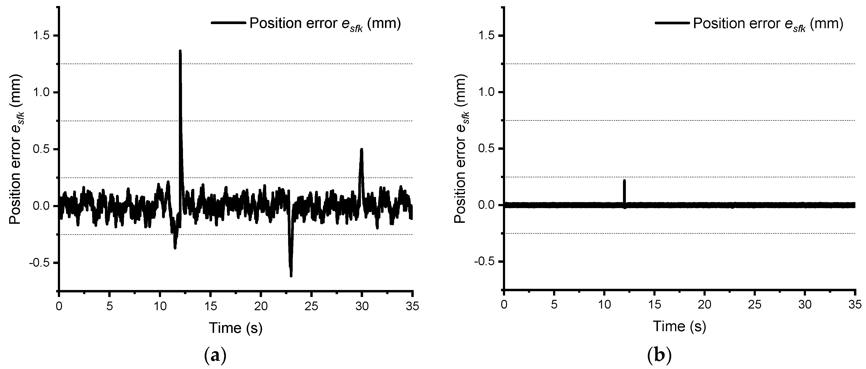
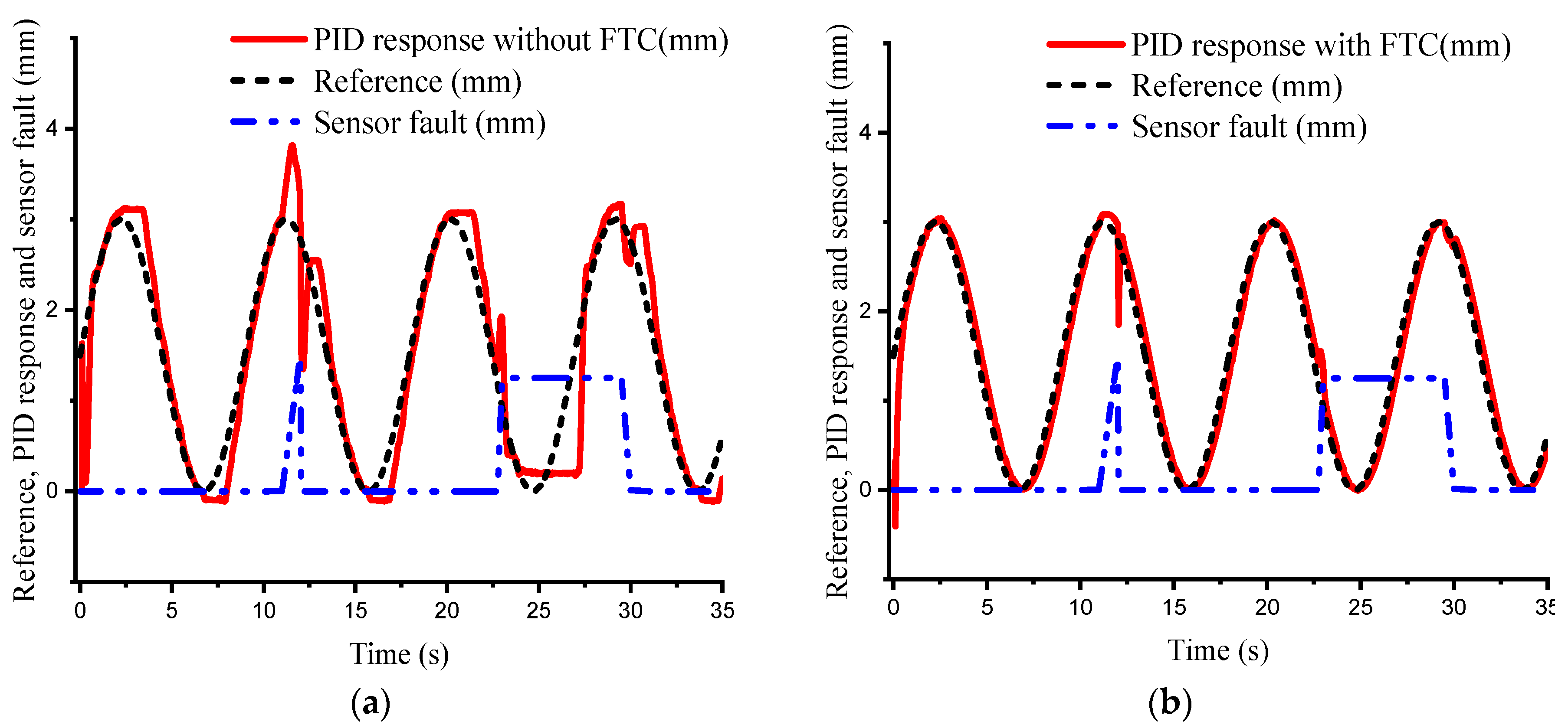
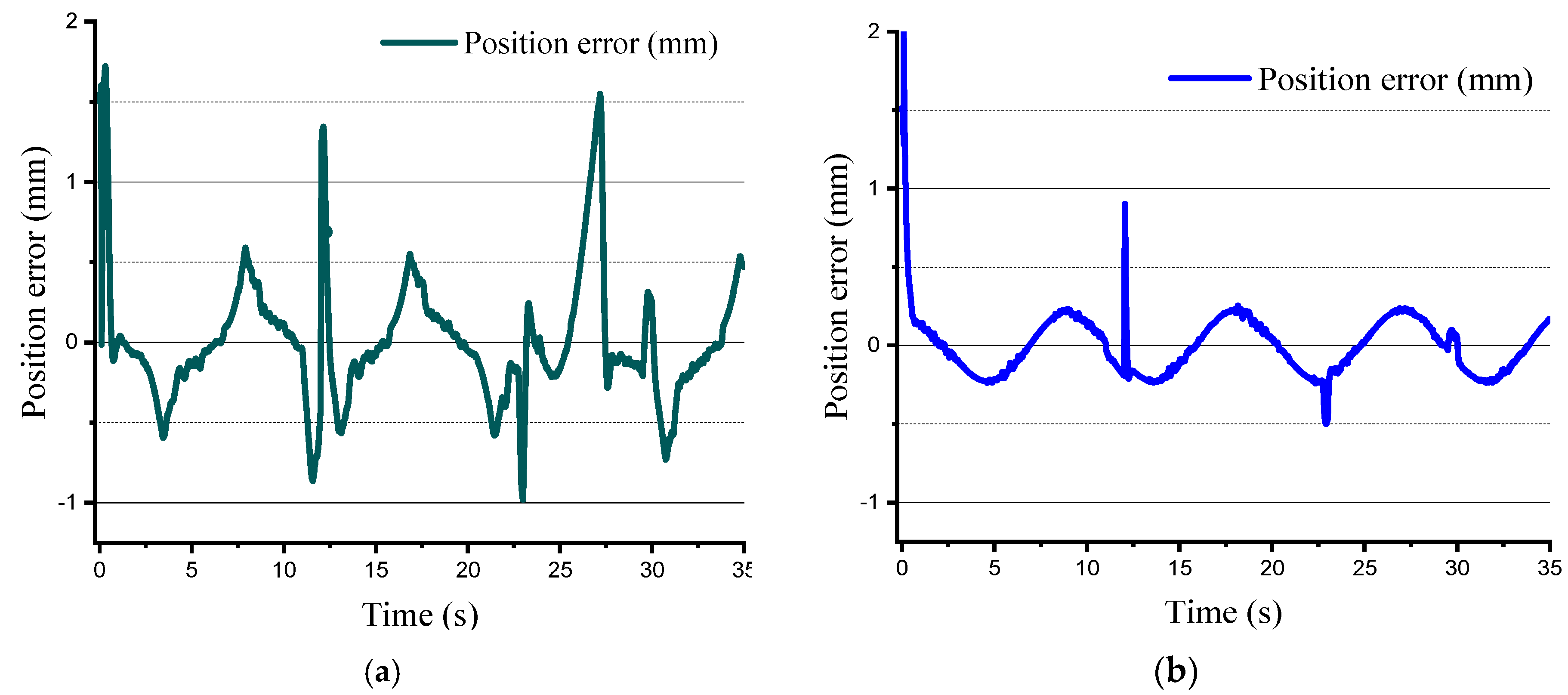
5.3. Experimental Results

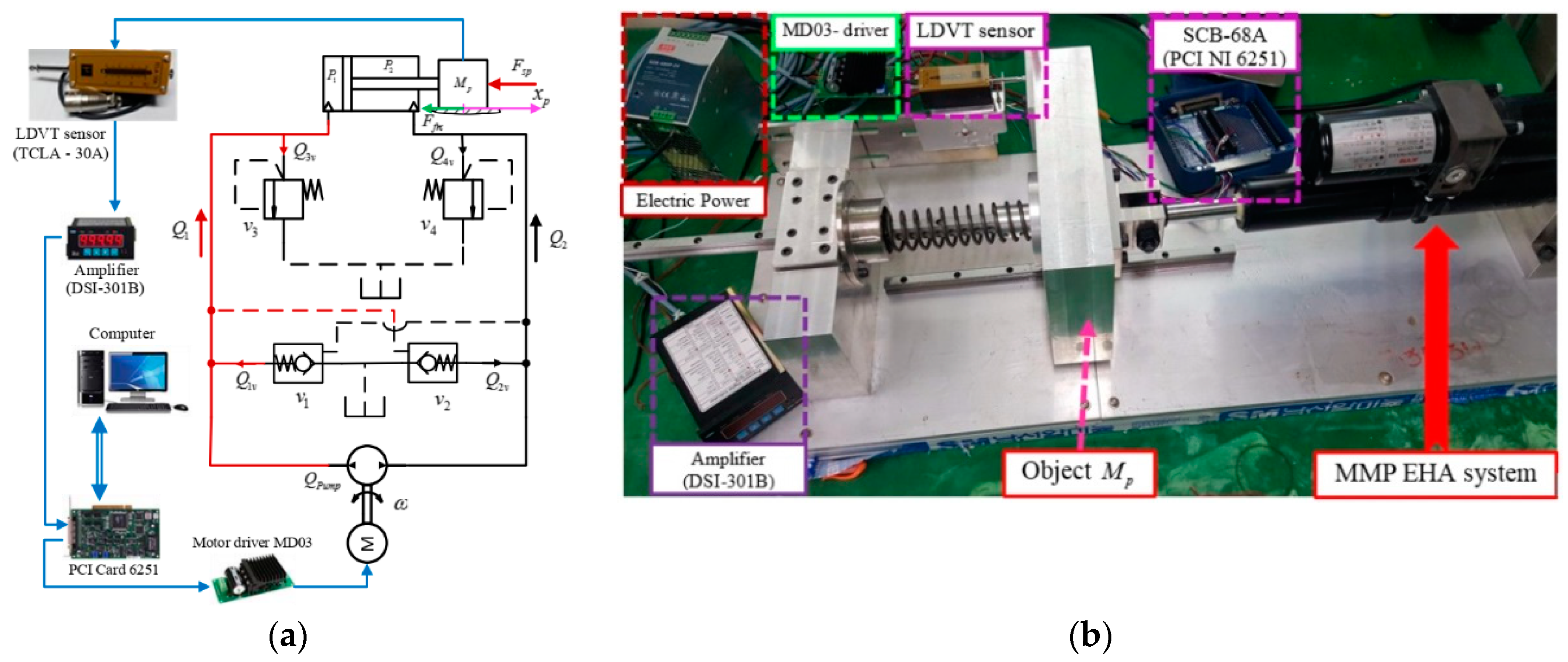
5.3.1. Diagram of the Testbed for the MMP System

In this section, the configuration of the EHA testbed setup is presented, where the EHA system includes a hydraulic cylinder, which is adjusted directly by operation of the bidirectional pump, as shown in Figure 12a. This means that changes in the cylinder speed depend on electric power shifts of the motor.

Therefore, to control the piston position of the cylinder, the relationship between electrical energy changes of the motor and piston position changes needs to be established. To do this, a linear variable differential transformer (LVDT) sensor is used to obtain data from the piston in the form of a digital signal. When the LVDT sensor TCLA-30A touches the surface of object Mp, as shown in Figure 12, the signal will be transferred to amplifier DSI-301B. Then, this signal will be transferred to the computer through a PCI card (NI 6251). Conversely, if the difference between the desired signal and the feedback signal from the LVDT sensor is zero, then the computer will send the analogue signal to the motor driver via PCI card NI 6251. As a result, the system operates under closed-loop control. The controller for the testbed is implemented on a personal computer (core 2 Duo 2.2 GHz) using Matlab Simulink version 2013b (32 bits) and the Real-time Windows Target Toolbox.

5.3.2. Results

SFTC experimental scheme of the MMP real system is performed using the setup shown in the diagram in Figure 12a,b. This technique is proposed to improve the performance of the PID controller for the MMP real system. The principle of this process is as follows. The feedback signals from the LVDT sensor signal where these sensor signals are filtered by a lowpass filter in combination with the mean value to smooth out the noise, which makes control easier. The experimental results were performed under a predetermined fault condition in (52) and the reference input in (51) for the MMP system. The results are shown in

Table 4. Evaluation of the error $e_{ck\max }$ using the PID controller.

Content	Sinusoidal Reference Signal
	Without FTC		With FTC
	${\mathit{e}}_{\mathit{c}\mathit{k}\mathbf{max}}\left(\mathit{mm}\right)$	${\mathit{\eta }}_{\mathit{k}}(\%)$	${\mathit{e}}_{\mathit{c}\mathit{k}\mathbf{max}}\left(\mathit{mm}\right)$	${\mathit{\eta }}_{\mathit{k}}(\%)$
From 0.5 s to 15 s	1.721	−4.74	0.903	39.80
From 15 s to 25 s	0.979	21.64	0.254	59.99
From 25 s to 35 s	1.550	−3.96	0.254	79.68
Average error performance from 0.5 s to 35 s	-	−5.69	-	59.82

. The value of the error performance ${\eta }_k$ for the case without SFTC was −5.69%, which indicates low performance. A negative value for the performance implies that the real system is affected by several faults, disturbances, and noises that are unknown.

The experimental results are shown in Figure 13. The PID position response signal is significantly improved when using the SFTC technique, as shown in Figure 14a,b. The effectiveness of this technique was evaluated using error performance ${\eta }_k$, as shown in Table 4. The differences between the average error performances are listed in Table 2 and 4 for the cases with and without SFTC, showing the effectiveness of the technique. Specifically, the control error performance ${\eta }_k$ is 59.82% for the case in which the SFTC technique was applied, which is shown in Figure 14a,b.

6. Discussion

In this paper, a mathematical model was developed based on [3]. In addition, a UIO based on the system reconstruction approach is applied to perform state and fault estimation. These techniques were studied and improved upon based on the proofs in previous papers [11,21]. Asymptotic stability of the state observer is guaranteed using the LMI optimization algorithm. Here, the numerical simulation process was conducted successfully on the MMP model. In particular, the SFTC technique was implemented effectively in the simulations and experiments. The experimental results showed that the position response in the case of SFTC was better than without SFTC. This performance of the applied SFTC resulted in an increase of 65.51% (from −5.69% to 59.82%) as shown in Table 4.

7. Conclusions

The SFTC technique was performed successfully in simulations and experiments for a nonlinear EHA system. The SFTC performance in simulations was approximately 93.78% in the case with a disturbance and 94.91% in the case without a disturbance. The fault and disturbance were nearly cancelled out when the SFTC technique was applied. In experiments using a real MMP system, the average performance was 59.82% when the SFTC technique was used. With the SFTC technique, the average performance increased by 65.51% (from −5.69% to 59.82%) and the control error improved, as shown in Table 4 and Figure 14a,b. Thus, the system can work well even when faults occur.

References

1. Samer, A.; Elmira, A.; Abdellatif, A.; Fethi, B.O.H.; Salem, A.N. Modeling and Simulation of a New Integrated Electrohydraulic Actuator for Humanoid Robots. Int. J. Adv. Robot. Automn. 2016, 1, 1–12. [Google Scholar] [CrossRef]
2. Xiang, L.; Zhen, C.Z.; Guang, C.R.; Dong, C.; Gang, S. Force Loading Tracking Control of an Electro-Hydraulic Actuator Based on a Nonlinear Adaptive Fuzzy Back-stepping Control Scheme. Symmetry 2018, 10, 155. [Google Scholar] [CrossRef]
3. Ahn, K.K.; Nam, C.N.D.; Jin, M. Adaptive Back-stepping Control of an Electrohydraulic Actuator. IEEE/ASME Trans. Mechatron. 2014, 19, 987–995. [Google Scholar] [CrossRef]
4. Shi, Z.; Tang, Z.; Pei, Z. Sliding Mode Control for Electro-hydrostatic Actuator. J. Control Sci. Eng. 2014, 2014. [Google Scholar] [CrossRef]
5. Marzat, J.; Piet-Lahanier, H.; Damongeot, F.; Walter, E. Model-based fault diagnosis for aerospace systems: A survey. Proc. Inst. Mech. Eng. G J. Aerosp. Eng. 2012, 226, 1329–1360. [Google Scholar] [CrossRef]
6. Mahulkar, V.; Adams, D.E.; Derriso, M. Adaptive fault tolerant control for hydraulic actuators. In Proceedings of the 2015 American Control Conference (ACC), Chicago, IL, USA, 1–3 July 2015; pp. 2242–2247. [Google Scholar] [CrossRef]
7. Liu, H.; Liu, D.; Lu, C.; Wang, X. Fault diagnosis of hydraulic servo system using the unscented Kalman filter. Asian J. Control 2014, 16, 1713–1725. [Google Scholar] [CrossRef]
8. Qingxian, J.; Huayi, L.; Yingchun, Z.; Xueqin, C. Robust observer-based sensor fault reconstruction for discrete-time systems via a descriptor system approach. Int. J. Control Autom. Syst. 2015, 13, 274. [Google Scholar] [CrossRef]
9. Liu, X.; Gao, Z.; Zhang, A. Robust Fault Tolerant Control for Discrete-Time Dynamic Systems with Applications to Aero Engineering Systems. IEEE Access 2018, 6, 18832–18847. [Google Scholar] [CrossRef]
10. Siti, F.A.L.; Abdul, R.H.; Mohamad, N.A.; Zaharuddin, M. Fault-Tolerant Control for Sensor Fault of a Single-Link Flexible Manipulator System. J. Teknol. 2016, 78, 6–13. [Google Scholar] [CrossRef]
11. Noura, H.; Theilliol, D.; Ponsart, J.C.; Chamseddine, A. Fault-Tolerant Control Systems Design, and Practical Applications; Michael, J.G., Michael, A.J., Eds.; Springer: Dordrecht, The Netherlans; Heidelberg, Germany; London, UK; New York, NY, USA, 2009; ISBN 978-1-84882-652-6. [Google Scholar] [CrossRef]
12. Nahian, S.A.; Truong, D.Q.; Chowdhury, P.; Das, D.; Ahn, K.K. Modeling and Fault Tolerant Control of an ElectroHydraulic Actuator. Int. J. Precis. Eng. Manuf. 2016, 17, 1285–1297. [Google Scholar] [CrossRef]
13. Bahareh, P.; Nader, M.; Khashayar, K. Sensor Fault Detection, Isolation, and Identification Using Multiple Model-based Hybrid Kalman Filter for Gas Turbine Engines. IEEE Trans. Control Syst. Technol. 2016, 24, 1184–1200. [Google Scholar] [CrossRef]
14. Fikret, C.; Chingiz, H. Active Fault-Tolerant Control of UAV Dynamics against Sensor-Actuator Failures. J. Aerosp. Eng. 2016, 29, 04016012. [Google Scholar] [CrossRef]
15. Gao, Z.; Breikin, T.; Wang, H. High-gain estimator and fault-tolerant design with application to a gas turbine dynamic system. IEEE Trans. Control Syst. Technol. 2007, 15, 740–753. [Google Scholar] [CrossRef]
16. Liu, X.; Gao, Z. Unknown input observers for fault diagnosis in Lipschitz nonlinear systems. In Proceedings of the 2015 IEEE International Conference on Mechatronics Automation (ICMA), Beijing, China, 2–5 August 2015; pp. 1555–1560. [Google Scholar] [CrossRef]
17. Noura, H.; Sauter, D.; Hamelin, F.; Theilliol, D. Fault-tolerant control in dynamic systems: Application to a winding machine. IEEE Control Syst. Mag. 2000, 20, 33–49. [Google Scholar] [CrossRef]
18. Han, W.; Zhang, Y.; Wang, Z.; Shen, Y. Robust fault estimation and accommodation for discrete-time Takagi-Sugeno fuzzy systems. In Proceedings of the 33rd Chinese Control Conference, Nanjing, China, 28–30 July 2014; pp. 3076–3081. [Google Scholar] [CrossRef]
19. Tabatabaeipour, M.; Bak, T. Robust observer-based fault estimation and accommodation of discrete-time piecewise linear systems. J. Frankl. Inst. 2013, 351, 277–295. [Google Scholar] [CrossRef]
20. Gao, Z. Fault Estimation and Fault-Tolerant Control for Discrete-Time Dynamic Systems. IEEE Trans. Ind. Electron. 2015, 62, 3874–3884. [Google Scholar] [CrossRef]
21. Shyamapda, M.; Sairam, N.; Sridhar, S.; Swaminathan, P. Nuclear power plant sensor fault detection using singular value decomposition-based method. Indian Acad. Sci. 2017, 42, 1473–1480. [Google Scholar] [CrossRef]
22. Jing, H.; Lin, M.; Songan, M.; Changfan, Z.; Houguang, C. Fault-Tolerant Control of a Nonlinear System Actuator Fault Based on Sliding Mode Control. J. Control Sci. Eng. 2017. [Google Scholar] [CrossRef]
23. Jian, Z.; Akshya, K.S.; Sing, K.N. Robust Observer-Based Fault Diagnosis for Nonlinear Systems Using MATLAB. In Advances in Industrial Control; Michael, J.G., Michael, A.J., Eds.; Springer International Publishing: Switzerland, 2016; ISBN 978-3-319-32323-7. [Google Scholar] [CrossRef]
24. Hmidi, R.; Brahim, A.B.; Hmida, F.B.; Sellami, A. Robust fault tolerant control for Lipschitz nonlinear systems with simultaneous actuator and sensor faults. In Proceedings of the 2018 International Conference on Advanced Systems Electric Technologies (IC_ASET), Hammamet, Tunisia, 22–25 March 2018; pp. 277–283. [Google Scholar] [CrossRef]
25. Shen, Q.; Jiang, B.; Shi, P. Fault Diagnosis and Fault-Tolerant Control Based on Adaptive Control Approach; Springer International Publishing AG: Cham, Switzerland, 2017; ISBN 978-3-319-52529-7. [Google Scholar] [CrossRef]
26. Robert, F.; David, H.; Catherine, C.; Eric, B. A Class of Nonlinear Unknown Input Observer for Fault Diagnosis: Application to Fault Tolerant Control of an Autonomous Spacecraft. In Proceedings of the 10th UKACC International Conference on Control (IEEE), Loughborough, UK, 9–11 July 2014; pp. 19–24. [Google Scholar] [CrossRef]
27. Gao, Z.; Ding, S.X. Sensor fault reconstruction and sensor compensation for a class of nonlinear state-space systems via a descriptor system approach. IET Control Theory Appl. 2007, 1, 578–585. [Google Scholar] [CrossRef]
28. Gao, Z.; Breikin, T.; Wang, H. Reliable Observer-Based Control Against Sensor Failures for Systems with Time Delays in Both State and Input. IEEE Trans. Syst. Man Cybern. Part A Syst. Hum. 2008, 38, 1018–1029. [Google Scholar] [CrossRef]
29. Tan, N.V.; Cheolkeun, H. Sensor Fault-Tolerant Control Design for Mini Motion Package Electro-Hydraulic Actuator. MDPI Process. 2019, 7, 89. [Google Scholar] [CrossRef]
30. Sami, M.; Patton, J.R. Active fault tolerant control for nonlinear systems with the simultaneous actuator and sensor faults. Int. J. Control Autom. Syst. 2013, 11, 1149. [Google Scholar] [CrossRef]
31. Gao, Z.; Liu, X.; Chen, Q.Z.M. Unknown Input Observer-Based Robust Fault Estimation for Systems Corrupted by Partially Decoupled Disturbances. IEEE Trans. Ind. Electron. 2016, 63, 2537–2547. [Google Scholar] [CrossRef] [Green Version]
32. Boyd, S.; Ghaoui, E.L.; Feron, E.; Balakrishnan, V. Linear Matrix Inequalities in Systems and Control Theory; SIAM: Philadelphia, PA, USA, 1994; ISBN 0-89871-334-X. [Google Scholar]
33. Zhang, J.; Zhao, X.; Zhu, F.; Karimi, H. Reduced-Order Observer Design for Switched Descriptor Systems with Unknown Inputs. IEEE Trans. Autom. Control 2019. [Google Scholar] [CrossRef]
34. Zhang, J.; Zhu, F.; Karimi, H.R.; Wang, F. Observer-based Sliding Mode Control for T-S Fuzzy Descriptor Systems with Time-delay. IEEE Tran. Fuzzy Syst. 2019. [Google Scholar] [CrossRef]
Figure 1. Schematic model of the EHA system.
Energies 12 04337 g001
Figure 2. Structure of the observer based on sensor fault-tolerant control.
Energies 12 04337 g002
Figure 3. Scheme to assess the control error of the PID controller using SFTC.
Energies 12 04337 g003
Figure 4. Position and estimate of position without FTC (a) disturbance d k = 0 , (b) disturbance d k .
Energies 12 04337 g004
Figure 5. Sensor fault and estimated fault without FTC: (a) disturbance d k   =   0 ; (b) disturbance d k .
Energies 12 04337 g005
Figure 6. Position and its estimation with FTC (a) disturbance d k   =   0 , (b) disturbance d k .
Energies 12 04337 g006
Figure 7. Sensor fault and estimated sensor fault with SFTC: (a) disturbance d k   =   0 and (b) disturbance d k .
Energies 12 04337 g007
Figure 8. The position control error e c k of the PID controller without disturbance d k for the cases: (a) without SFTC, (b) with SFTC.
Energies 12 04337 g008
Figure 9. The position control error e s f k of the PID controller without disturbance d k for the case: (a) without SFTC, (b) with SFTC.
Energies 12 04337 g009
Figure 10. The position control error e c k for the case with disturbance d k for the case: (a) without SFTC, (b) with SFTC.
Energies 12 04337 g010
Figure 11. The position control error e c k for the case with disturbance d k for the case: (a) without SFTC, (b) with SFTC.
Energies 12 04337 g011
Figure 12. The testbed for the EHA system: (a) structure of the testbed for the EHA system, (b) experimental EHA testbed.
Energies 12 04337 g012
Figure 13. PID position response and an estimate of position: (a) without FTC, (b) with FTC.
Energies 12 04337 g013
Figure 14. PID position error in the experiment: (a) the case without SFTC, (b) the case with SFTC.
Energies 12 04337 g014