Neutral-Point Potential Balancing Control Strategy for Three-Level ANPC Converter Using SHEPWM Scheme

Abstract

A selective harmonic elimination pulse width modulation (SHEPWM) control strategy is proposed to balance the neutral-point potential (NP) of a three-level active neutral-point-clamped (ANPC) converter. In this strategy, the chaotic ant colony algorithm (ACA) is adopted to solve the SHEPWM nonlinear equations, which does not require presetting the initial values of solutions and can get multiple solutions in the same modulation index. The influence of different solutions corresponding to the SHEPWM switching states on the NP is different, namely, some make the NP increase and others make the NP decrease. Therefore, the NP balancing can be effectively controlled by choosing appropriate solutions in different fundamental periods. The simulation and experimental results further verify the feasibility and effectiveness of the control strategy.

1. Introduction

The multi-level converters have a wide utilization in new energy power generation and high-voltage power electronic devices. The neutral-point-clamped (NPC) converter has a wide utilization in multilevel topology since its invention in 1981 [1]. The application of the NPC converter is limited due to the unbalanced distribution of switching losses. Compared with the NPC topology, active neutral-point-clamped (ANPC) topology was introduced to the balanced loss distribution by choosing an appropriate NPC path [2], thus improving the switching frequency and output power in the converter [3].

The main disadvantage of the three-level (3L) NPC converter is the unbalance of neutral-point potential (NP) [4]. The unbalance of the NP will increase the output harmonics of the converter. The NP control strategy is divided into two kinds, which are adding a hardware circuit and using a control algorithm. Many adding hardware circuit methods have been proposed to control the NP [5,6,7]. All of them have been implemented by increasing hardware cost and complexity. Instead of changing hardware, the control algorithms have been used to control the NP in the converters [8]. These control algorithms are generally based on a variety of pulse width modulation (PWM) methods, such as carrier-based sinusoidal PWM (SPWM) [9,10], space vector (SV) PWM [11,12,13], selective harmonic elimination (SHE) PWM [14].

The SHEPWM has the advantages of small order harmonic spectrum and low switching frequency [14]. However, many non-idealities can cause the variation of the NP, such as inaccuracy in switching instants, component imperfections and other [15]. The SHEPWM method has difficulty in solving nonlinear transcendental equations, so it is difficult to realize on-line control. This disadvantage limits the commercial application of the SHEPWM method. There are three main methods used in SHEPWM: Numerical methods, algebraic methods, and evolutionary algorithms (EAS) [16]. Numerical methods include gradient optimization, sequential quadratic programming, and Newton–Raphson (NR), etc. [17]. However, the biggest problem of numerical methods is that they are heavily dependent on the selection of initial value and cannot find all possible solutions [18]. Although these problems can be overcome by algebraic methods, such as the synthetic elimination method and the Grobner basis method, their calculation is too complex. However, in the process of converter operation, the modulation index varies, and the solutions of the SHEPWM equations are the function of the modulation index. Therefore, it is difficult to preset the initial values exactly over the whole modulation index for real application. In the third kind of algorithm, such as genetic algorithm (GA), bee algorithm (BA) and chaos ant colony algorithm (ACA) are easy to realize and they are less affected by initial guesses when finding the optimal solutions [19]. These algorithms have different concepts and structures.

In this paper, a control strategy using SHEPWM is proposed to balance the NP of a 3L-ANPC converter. In this strategy, the chaotic ant colony algorithm (ACA) is used to solve the SHEPWM transcendental equations. Using ACA for solving the SHEPWM nonlinear equations, it does not need presetting initial values of the solutions and can get multiple solutions in the same modulation index. The influence of different solutions on the NP is different. It is found that some solutions make the NP up, and others make the NP down. By selecting a set of appropriate switching angles in next fundamental period according to the NP offset in current fundamental period, the selective harmonic is eliminated and the NP self-balancing is enhanced.

This article elaborates on the following aspects. The operating principle of the 3L-ANPC converter is introduced in Section 2, In Section 3, the chaotic ant colony algorithm and the method of solving the SHEPWM equations are proposed. The control strategy of the NP balancing is proposed in Section 4. In Section 5, simulation and experimental results are presented to validate the proposed method, and finally, conclusions are summarized in Section 6.

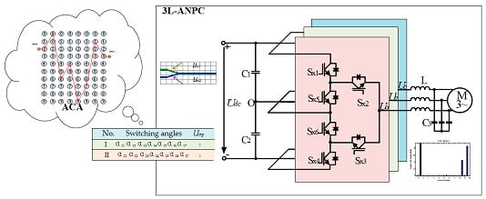
2. 3L-ANPC Converter and SHEPWM

Firstly, the structure and switching state of three-level ANPC inverters are introduced. Then the equation for eliminating specific harmonics of three-level inverters is introduced. By solving the equation, the switching angles of SHEPWM can be obtained.

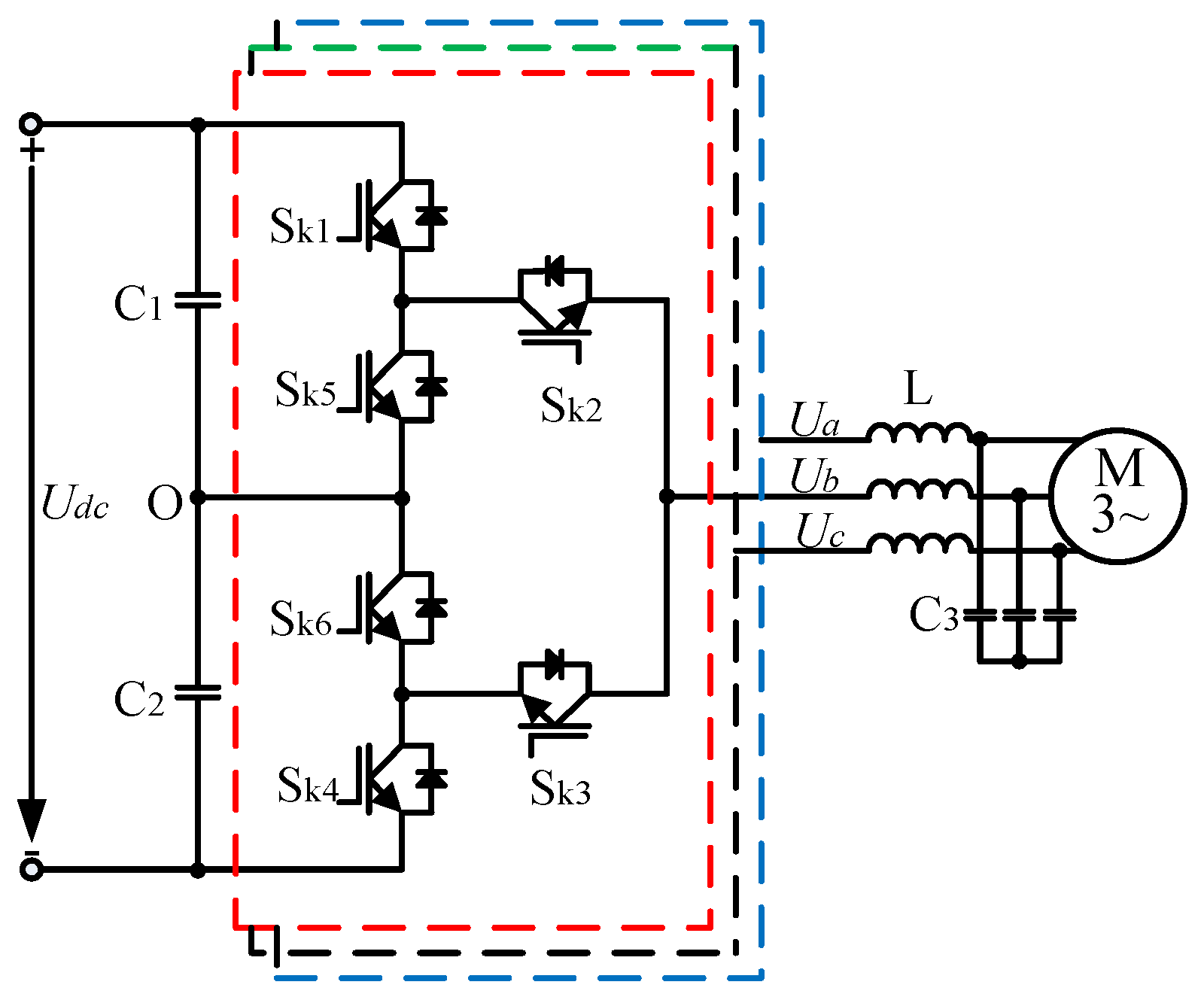
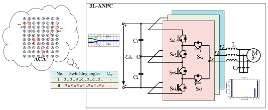
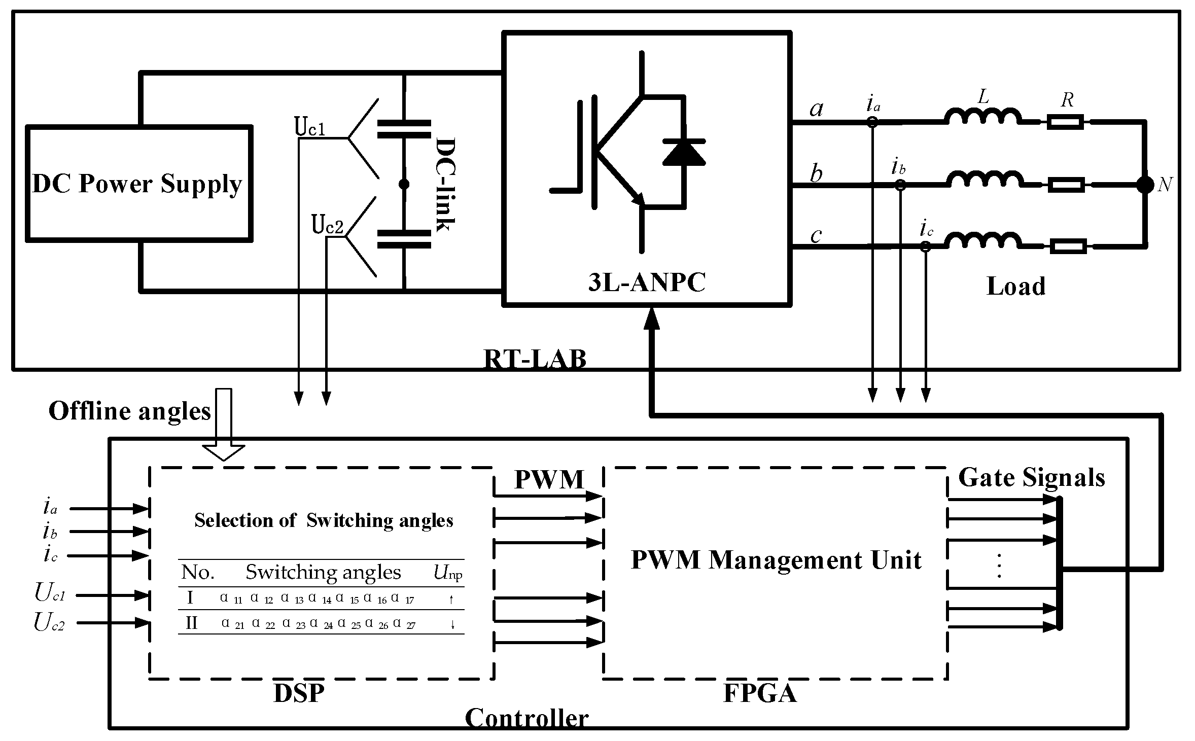
2.1. Principle of 3L-ANPC Converter

The simplified circuit diagram of the three-phase 3L-ANPC converter can be seen in Figure 1, The two dc-link capacitors (C₁ and C₂) should share equally the dc-link voltage (U_dc) and the dc-link is shared by three-phase legs. Each phase-leg is composed of six switch devices (S_k1, S_k2, S_k3, S_k4, S_k5, and S_k6), where k can be the three-phases a, b or c. The voltage of the neutral-point of dc-link is regarded as zero potential, each phase-leg can produce three different levels of U_dc/2, 0 and –U_dc/2, which are called P, O, and N states, respectively. The current paths of P and N states are similar to those of NPC topology. Because S_k2, S_k3 are active switch devices, there are two additional current paths at zero level, the current of the O state can be through the S_k2, S_k5, and it can also be through the S_k3, S_k6 [2]. There are four redundant switching states at zero-level O state: OU1, OU2, OL1, and OL2. The six switching states of the 3L-ANPC converter are shown in

Table 1. Switching states of 3L-ANPC converter.

Switches						Phase Voltage	Switching State
Sk1	Sk2	Sk3	Sk4	Sk5	Sk6
1	1	0	0	0	1	Udc/2	P
0	1	0	0	1	0	0	OU1
0	1	0	1	1	0	0	OU2
0	0	1	0	0	1	0	OL1
1	0	1	0	0	1	0	OL2
0	0	1	1	1	0	–Udc/2	N

. The loss distribution of devices can be controlled by selecting different zero-level states. Their detailed discussion can be found in [3].

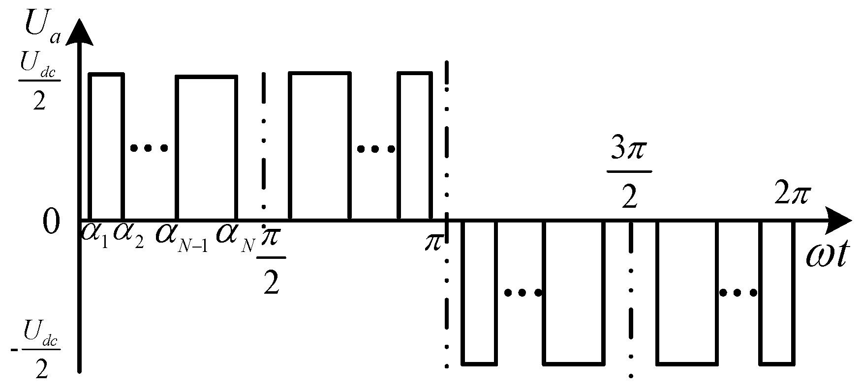
2.2. Three-Level SHEPWM

Figure 2 shows the three-level line-to-neutral waveform based on the SHEPWM method, where the switching angles of the SHEPWM are ${\alpha }_1$, ${\alpha }_2$, ${\alpha }_3$, …, ${\alpha }_N$ respectively, and N is the number of switching transitions in the1/4 fundamental period.

According to the Dirichlet theorem, the following Fourier series can be obtained.

$$U_{AN}(\omega t)={\displaystyle \sum _{n=1}^{\infty }[A_n\cos (n\omega t)+B_n\sin (n\omega t)]}$$

(1)

where, A_n and B_n are the Fourier coefficients.

The SHEPWM waveform is odd- and half-wave symmetries, so the Fourier coefficients can be calculated as the following

$$\{\begin{array}{c}{A}_n=0\\ B_n=\{\begin{array}{l}0,n=even\\ =\frac{2U_{dc}}{n\pi }{\displaystyle \sum _{k=1}^N{(-1)}^{k+1}\cos (n{\alpha }_k),n=odd}\end{array}\end{array}$$

(2)

where N is the number of switching transitions within the 1/4 fundamental period, and ${\alpha }_1$, ${\alpha }_2$, ${\alpha }_3$, …, ${\alpha }_N$ satisfy Formula (3).

$$0<{\alpha }_1<{\alpha }_2<\cdots <{\alpha }_{N-1}<{\alpha }_N<\frac{\pi }{2}$$

(3)

In a three-phase system, the zero-sequence harmonic can be eliminated, so by selecting the optimal switching angles ${\alpha }_1$, ${\alpha }_2$, ${\alpha }_3$, …, ${\alpha }_N$ the 5th, 7th, 11th, 13th,…, (6i ± 1)th order harmonics can be eliminated through (4), where i is positive integer.

$$\{\begin{array}{l}{f}_1(\alpha )=\frac{4}{\pi }{\displaystyle \sum _{i=1}^N{(-1)}^{i+1}\cos ({\alpha }_i)}=\cdots \\ f_2(\alpha )=\frac{4}{5\pi }{\displaystyle \sum _{i=1}^N{(-1)}^{i+1}\cos (5{\alpha }_i)=0}\\ ⋮\\ f_N(\alpha )=\frac{4}{l\pi }{\displaystyle \sum _{i=1}^N{(-1)}^{i+1}\cos (l{\alpha }_i)=0}\end{array}$$

(4)

where l is the highest order of harmonics to be eliminated and m is the fundamental modulation index and calculated by

$$m=\frac{B_1}{U_{dc}/2}$$

(5)

Equations (4) are transcendental, and therefore, multiple solutions are exhibited at the same modulation index. By solving the equation, the switching angles, which can eliminate the selected low-order harmonics can be obtained.

If different numerical algorithms are used to solve the SHEPWM equation, the initial values must be preset and the trend of these values in the whole range of modulation index must be predicted. As mentioned above, the preset of initial values is difficult in the real application. In order to solve this problem, the chaotic ACA is used in this paper, because it has the inherent ability to start random search and process a large amount of data simultaneously.

3. Chaotic Ant Colony Algorithm and Solving SHEPWM Equation

This part includes two parts: (1) Variable-scale chaotic ant colony algorithm, (2) solving SHEPWM nonlinear equations. The application of the chaotic ant colony algorithm in solving SHE nonlinear equation is introduced.

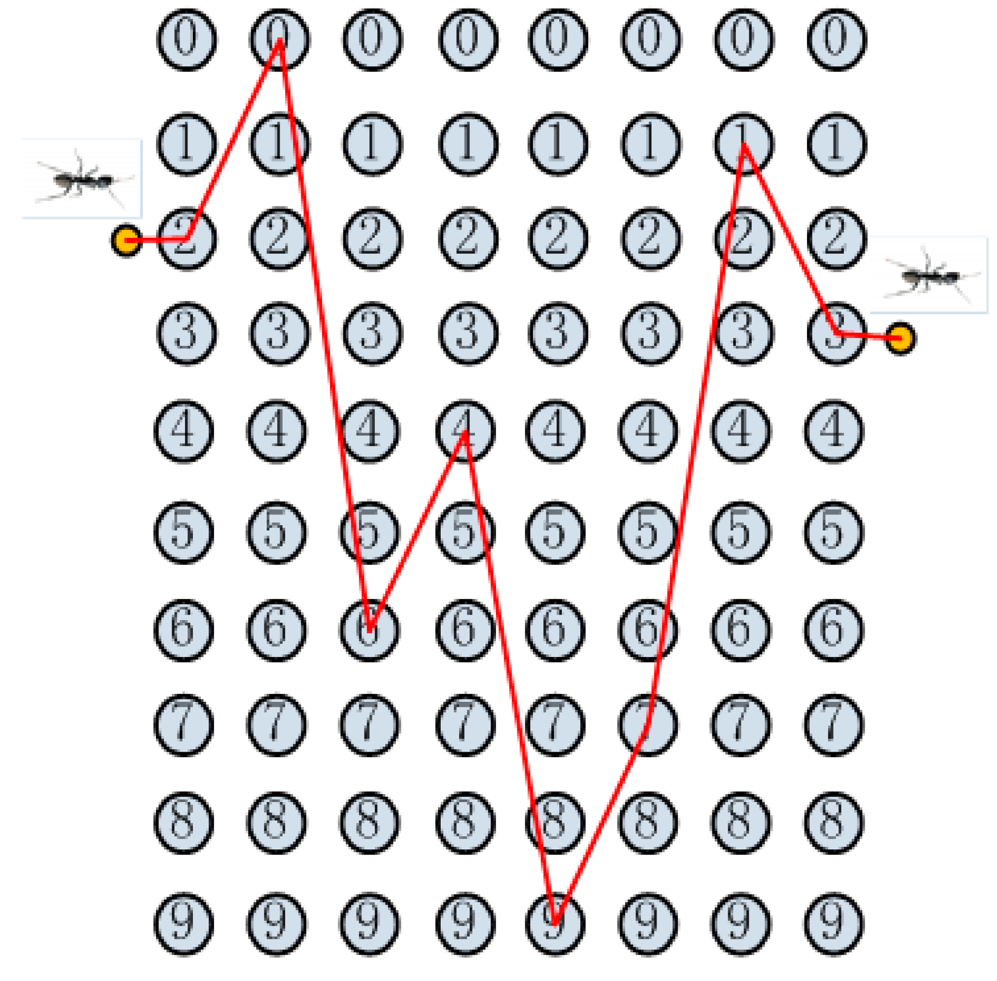
3.1. Variable-scale Chaotic Ant Colony Algorithm

Inspired by the ant food searching behaviors, ACA is proposed by Marco Dorigo et al. [20]. Ants have great construction and organization abilities by the colony behaviors. The most attractive part of their behavior is how they look for food, and how ants choose the shortest path between their nest and the food sources. When looking for food, initially, ants search around the nest in a random way. While ants walk back and forth between nests and food sources, they leave some chemical pheromone on the ground. The quality of the food source and the length of the path determine the quantity of pheromones. Ants can choose a precise path according to the intensity of pheromone. The concentration of pheromone increased with the number of ants choosing the path. Therefore, the ants can use the pheromone concentration to find the nearest food source [21,22].

The optimized function variable can be expressed as a decimal string $d(0),d(1),\dots ,d(l-1)$.

Decoding formula of the node i as follows [23],

$$X_i={\displaystyle \sum _{i=0}^{1/n}d((i*1/n+b)*{10}^{-b})}$$

(6)

where i is the number of current locating layers, b is the length of strings, n is the dimension of variables.

The process represented by the formula can be shown in Figure 3.

As seen from Figure 3, when the ants from one layer to another, they will have ten choices.

When the solution construction is completed, the ants provide feedback to the solutions by depositing pheromones on solution components, for which they use the updating rule in their solution.

Because ants take different routes, local updating pheromone of each ant is different. Locally update the initial pheromone of ants as shown [23],

$${\tau }_{ij}(t+1)=(1-\rho ){\tau }_{ij}(t)+\rho {\tau }_0$$

(7)

where ${\tau }_{ij}$ is the pheromone trail deposited between node i and j, ${\tau }_0$ is the initial pheromone level, and ρ is the evaporation parameter ($0<\rho <1$).

Due to the attraction of ants to this path, the pheromone content is the strongest in the best path. At the same time, the pheromones on other paths evaporate in time. When all ants complete a path, by using the following [23], the global pheromone level is updated.

$${\tau }_{ij}(t+1)=(1-\alpha ){\tau }_{ij}(t)+\alpha \tau /f_{best}$$

(8)

where $\alpha$ is the pheromone decay parameter ($0<\alpha <1$), and $f_{best}$ is the function value of global optimal ant.

Using chaotic factor instead of random factor, the efficiency of the stochastic optimization algorithm is improved. The chaotic mapping can be regarded as a non-linear differential equation without any stochastic factors, but its trajectory is completely stochastic and ergodic in the state space. The most common Logistic mapping in this paper is adopted, which can be described as follows [24],

$$x_{n+1}(t+1)=\mu x_n(1-x_n)$$

(9)

where $x$ is a chaotic variable ($0<x<1$), and $\mu$ is a constant ($0<\mu \le 4$).

When the chaotic mapping is used in ACA, the initialization parameter is chaos. Each chaotic parameter corresponds to a path, so there are many paths. Some better paths with the inverse pheromone can be selected. Therefore, in order to speed up convergence, the pheromones of each path are not equal.

The variable-scale chaotic ACA can be described as follows [23].

(1)

A chaotic series are embedded into the solutions getting from ACA. After all ants have completed solution construction, the global best ant will be evaluated. The chaos optimization algorithm is used to search within a certain radius of the independent variable of the best ant, and the search radius will be reduced with the iteration. If a better solution is found, it will be decoded into a string of decimal numbers and replaced the best ant.

(2)

In order to search only nearby the best ant, the interval of chaotic series is transformed from (0, 1) to (−r, r) by a linear transformation. Then, the transformed series are embedded into the solution getting from the best ant, so new series are found.

(3)

The last is a variable radius problem. By adding the variable-scale algorithm to the chaotic ACA, the search scope can expand at the start stage to avoid getting into local optimum, at the same time, it can narrow the search scope at the later stage, so as to improve the search precision.

The variable-scale formula is used by Sigmoid formula [23], as follows,

$$r(t)=1-\frac{1}{1+\exp (-0.02t+4)}$$

(10)

The steps of variable-scale chaotic ACA are as follows,

Step 1 Initialization. Some parameters of the algorithm are initialized, such as number of ants, number of nodes, the maximum distance for each ant’s tour, maximum iteration, evaporation parameter, pheromone decay parameter, initial pheromone level, etc.

Step 2 The first position is provided at random.

Step 3 Select nodes according to the node selection rule.

Step 4 Local pheromone updating by formula (6).

Step 5 The value of independent variable is obtained by the formula (5), and the function value is calculated.

Step 6 The best ant is selected in current iteration. If it is superior to the global best ant, replace it.

Step 7 Calculate the chaotic searching radius using formula (9).

Step 8 Chaotic search nearby the global best ant. If a better solution than the global best ant can be found, and replace it.

Step 9 Global pheromone updating by formula (7).

Step 10 Return to step 2, do until the best solution is obtained or the maximum iteration is reached, then program stop.

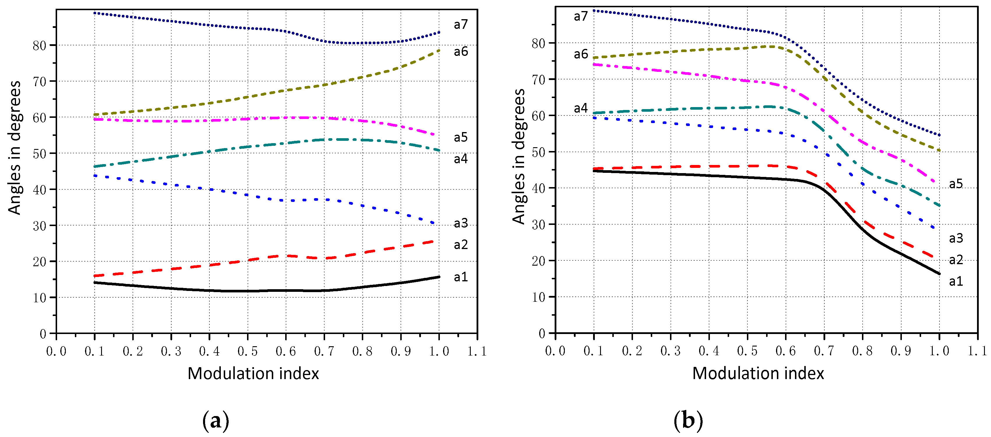
3.2. Solving SHEPWM Nonlinear Equations

The variable-scale chaotic ACA is applied, so as to solve the SHEPWM nonlinear equations in this paper. Compared with the traditional numerical method, it does not need preset initial values of the solutions and can obtain multiple solutions in the same modulation index.

According to Equation (4) can be obtained as follows,

$$\{\begin{array}{l}{g}_1=(\frac{4}{\pi }{\displaystyle \sum _{i=1}^N{(-1)}^{i+1}\cos ({\alpha }_i)}-m{)}^2\\ g_2=(\frac{4}{5\pi }{\displaystyle \sum _{i=1}^N{(-1)}^{i+1}\cos (5{\alpha }_i){)}^2}\\ ⋮\\ g_N=(\frac{4}{M\pi }{\displaystyle \sum _{i=1}^N{(-1)}^{i+1}\cos (M{\alpha }_i){)}^2}\end{array}$$

(11)

where $g_1$, $g_2$,…$g_{\mathrm{N}}$ are objective functions.

Let the minimum values of the objective functions tend to zero, and find the optimal switching angles to achieve the purpose of optimization.

According to the objective, the function is defined as follows:

$$g=-\frac{1}{1+g_1+g_2+\dots g_n}$$

(12)

Take g as the objective function to be optimized, the approximate solutions of the Equations (4) can be obtained by using the variable-scale ACA.

In this paper, we take the four angles within the first quarter cycle as an example, (i.e., N = 7), to eliminate 5th, 7th, 11th, 13th, 17th, and 19th harmonics.

Using the above method, a lot of switch angles can be obtained, in which two sets of switching angle tracks within the whole modulation index range are shown in Figure 4.

4. Control Strategy of NP Balancing

Firstly, the effect on NP with different SHEPWM switching angles is explained. Using the variable-scale chaotic ACA mentioned in the previous part, different switching groups with different influences on NP can be obtained under the same modulation degree. According to the need of neutral point balance, the appropriate SHEPWM switching groups are selected in the next fundamental period, and the neutral point control factor H is introduced. the amplitude of NP will be controlled within a certain extent of the dc-side voltage.

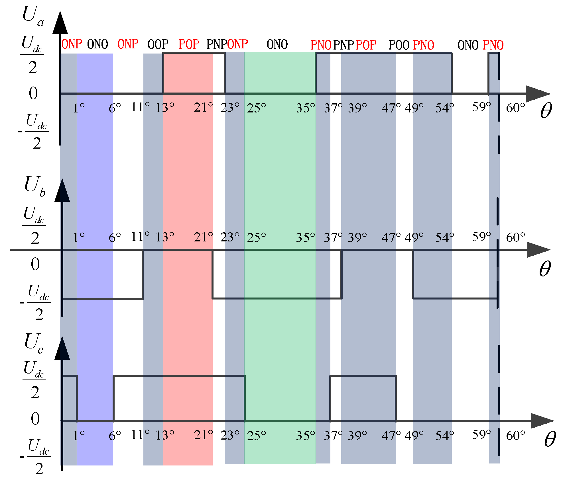
4.1. Effect on NP with Different SHEPWM Switching Angles

To explain the control strategy proposed, the number of switching transitions is chosen to be seven in 1/4 fundamental period. As shown in Figure 4a, when the modulation index is 0.8, the switch angles are α₁ = 13°, α₂ = 23°, α₃ = 35°, α₄ = 54°, α₅ = 59°, α₆ = 71°, and α₇ = 80° respectively. For simplicity, the numbers after the decimal point of the switch angles are ignored. Three-phase SHEPWM output within 1/4 of the fundamental period is shown in Figure 5. The three-phase output can be considered as switching state vectors. For example, three-phase waveforms in the blue region from 1° to 6° can be represented by the switching state vector ONO, and the three-phase waveforms in the red region from 39° to 47° can be expressed as the switching state vector POP.

Table 2. Vectors of SHEPWM and their duration time in 1/4 period.

Duration range	0°–1°	1°–6°	6°–11°	11°–13°
Switching state vector	ONP	ONO	ONP	OOP
Duration range	21°–23°	23°–25°	25°–35°	35°–37°
Switching state vector	PNP	ONP	ONO	PNO
Duration range	39°–47°	47°–49°	49°–54°	54°–59°
Switching state vector	POP	POO	PNO	ONO

shows all possible switching state vectors of SHEPWM and their duration from 0° to 60°. According to the symmetry of the SHEPWM waveform, all switching state vectors can be obtained within the whole fundamental period.

According to the above analysis, the switching state vectors of three-phase SHEPWM include large, medium, small vector and zero vector.

Define the switching states of the 3L-ANPC converter as $S_k=[S_a,S_b,S_c]$,

$$S_k=\{\begin{array}{c}1\begin{array}{cc},& \mathrm{Phase}\mathrm{k}\mathrm{output}\mathrm{is}\mathrm{P}\end{array}\\ 0\begin{array}{cc},& \mathrm{Phase}\mathrm{k}\mathrm{output}\mathrm{is}\mathrm{O}\end{array}\\ -1\begin{array}{cc},& \mathrm{Phase}\mathrm{k}\mathrm{output}\mathrm{is}\mathrm{N}\end{array}\end{array}\begin{array}{cc}& k=a,b,c\end{array}$$

(13)

Three-phase output voltage can be expressed as,

$$\{\begin{array}{c}{U}_{ao}=\frac{1}{2}{U}_{dc}\cdot S_a\\ U_{bo}=\frac{1}{2}{U}_{dc}\cdot S_b\\ U_{co}=\frac{1}{2}{U}_{dc}\cdot S_c\end{array}$$

(14)

The transient value of neutral point current $i_{np}(t)$ is calculated by,

$$i_{np}(t)=-(\left|S_a(t)\right|i_a(t)+\left|S_b(t)\right|i_b(t)+\left|S_c(t)\right|i_c(t))$$

(15)

where $i_a(t)$, $i_b(t)$, $i_c(t)$ are the instantaneous output current values of phase a, b and c, respectively.

For three-level inverters, the NP balancing is important. Among the large, medium, small, and zero vectors, only the medium and small vectors affect the NP equilibrium, and small vectors appear in pairs. The positive and negative small vectors in a pair of small vectors have opposite effects on the neutral point.

When the phase current i_k(t) (k = a, b, or c) flows from the converter to the load, it can be assumed that the current is positive. The effects of the small, medium vectors on the neutral point current are shown in

Table 3. Effect on neutral point current with medium vectors and small vectors.

Small Vector	${\mathit{i}}_{\mathit{n}\mathit{p}}(\mathit{t})$	Small Vector	${\mathit{i}}_{\mathit{n}\mathit{p}}(\mathit{t})$	Medium Vector	${\mathit{i}}_{\mathit{n}\mathit{p}}(\mathit{t})$
POO	$-i_a(t)$	ONN	$i_a(t)$	PON	$i_b(t)$
PPO	$i_c(t)$	OON	$-i_c(t)$	OPN	$i_a(t)$
OPO	$-i_b(t)$	NON	$i_b(t)$	NPO	$i_c(t)$
OPP	$i_a(t)$	NOO	$-i_a(t)$	NOP	$i_b(t)$
OOP	$-i_c(t)$	NNO	$i_c(t)$	ONP	$i_a(t)$
POP	$i_b(t)$	ONO	$-i_b(t)$	PNO	$i_c(t)$

. The effect of the small, medium vectors on NP voltage is shown in

Table 4. Influences of small and medium vectors on NP.

Positive Small Vectors	${\mathit{u}}_{\mathit{n}\mathit{p}}(\mathit{t})$	Negative Small Vectors	${\mathit{u}}_{\mathit{n}\mathit{p}}(\mathit{t})$	Medium Vectors	${\mathit{u}}_{\mathit{n}\mathit{p}}(\mathit{t})$
ONN	↑	POO	↓	PON	↑
PPO	↑	OON	↓	OPN	↑
NON	↑	OPO	↓	NPO	↑
OPP	↑	NOO	↓	NOP	↑
NNO	↑	OOP	↓	ONP	↑
POP	↑	ONO	↓	PNO	↑

. Therefore, the effect on the NP with different SHEPWM switching angles can be calculated.

The three-phase current of the 3L-ANPC converter is shown in (16).

$$\{\begin{array}{l}{i}_a(t)=I_m\cdot \sin (\omega t+\varphi )\begin{array}{cc}& \end{array}\\ i_b(t)=I_m\cdot \sin (\omega t+\varphi -\frac{2}{3}\pi )\\ i_c(t)=I_m\cdot \sin (\omega t+\varphi +\frac{2}{3}\pi )\end{array}$$

(16)

where $\phi$ is the power factor angle.

Define U_np as the NP offset in a fundamental period. U_np is affected by discharging energy and charging energy of C₁, C₂, which depend on the waveform of the three-phase and the current. U_np is calculated by,

$$U_{\mathrm{np}}==\frac{1}{C_2}{\displaystyle {\int }_{0^{\circ }}^{{360}^{\circ }}x(t)i_a(t)+y(t)i_b(t)+z(t)i_c(t)}dt$$

(17)

where $x(t)$, $y(t)$, $z(t)$ are the coefficients of $i_a(t)$, $i_b(t)$, $i_c(t)$, respectively.

$$\begin{array}{l}x(t)=\{\begin{array}{c}\begin{array}{cc}1& \mathrm{when}\mathrm{phase}\mathrm{a}\mathrm{output}\mathrm{O}\end{array}\\ \begin{array}{cc}0& \mathrm{when}\mathrm{phase}\mathrm{a}\mathrm{ouput}\mathrm{P},\mathrm{N}\end{array}\end{array}\\ y(t)=\{\begin{array}{c}\begin{array}{cc}1& \mathrm{when}\mathrm{phase}\mathrm{b}\mathrm{output}\mathrm{O}\end{array}\\ \begin{array}{cc}0& \mathrm{when}\mathrm{phase}\mathrm{b}\mathrm{ouput}\mathrm{P},\mathrm{N}\end{array}\end{array}\\ z(t)=\{\begin{array}{c}\begin{array}{cc}1& \mathrm{when}\mathrm{phase}\mathrm{c}\mathrm{output}\mathrm{O}\end{array}\\ \begin{array}{cc}0& \mathrm{when}\mathrm{phase}\mathrm{c}\mathrm{ouput}\mathrm{P},\mathrm{N}\end{array}\end{array}\end{array}$$

(18)

Because Equation (4) has multiple solutions at the same modulation index, multiple switching-state vectors of SHEPWM can be chosen. On the basis of the modulation index, the output current and power factor, two sets of the switching angles can be selected, which have different effects on NP, and there is a set of the switching angles that make the NP increase, others make the NP decrease.

Table 5. Effect on NP with different switching angles.

No.	Switching Angles					Unp
I	${\mathsf{\alpha }}_{11}$	${\mathsf{\alpha }}_{12}$	${\mathsf{\alpha }}_{13}$	…	${\mathsf{\alpha }}_{1\mathrm{N}}$	↑
II	${\mathsf{\alpha }}_{21}$	${\mathsf{\alpha }}_{22}$	${\mathsf{\alpha }}_{23}$	…	${\mathsf{\alpha }}_{2\mathrm{N}}$	↓

shows the effects of different switching angles on the NP.

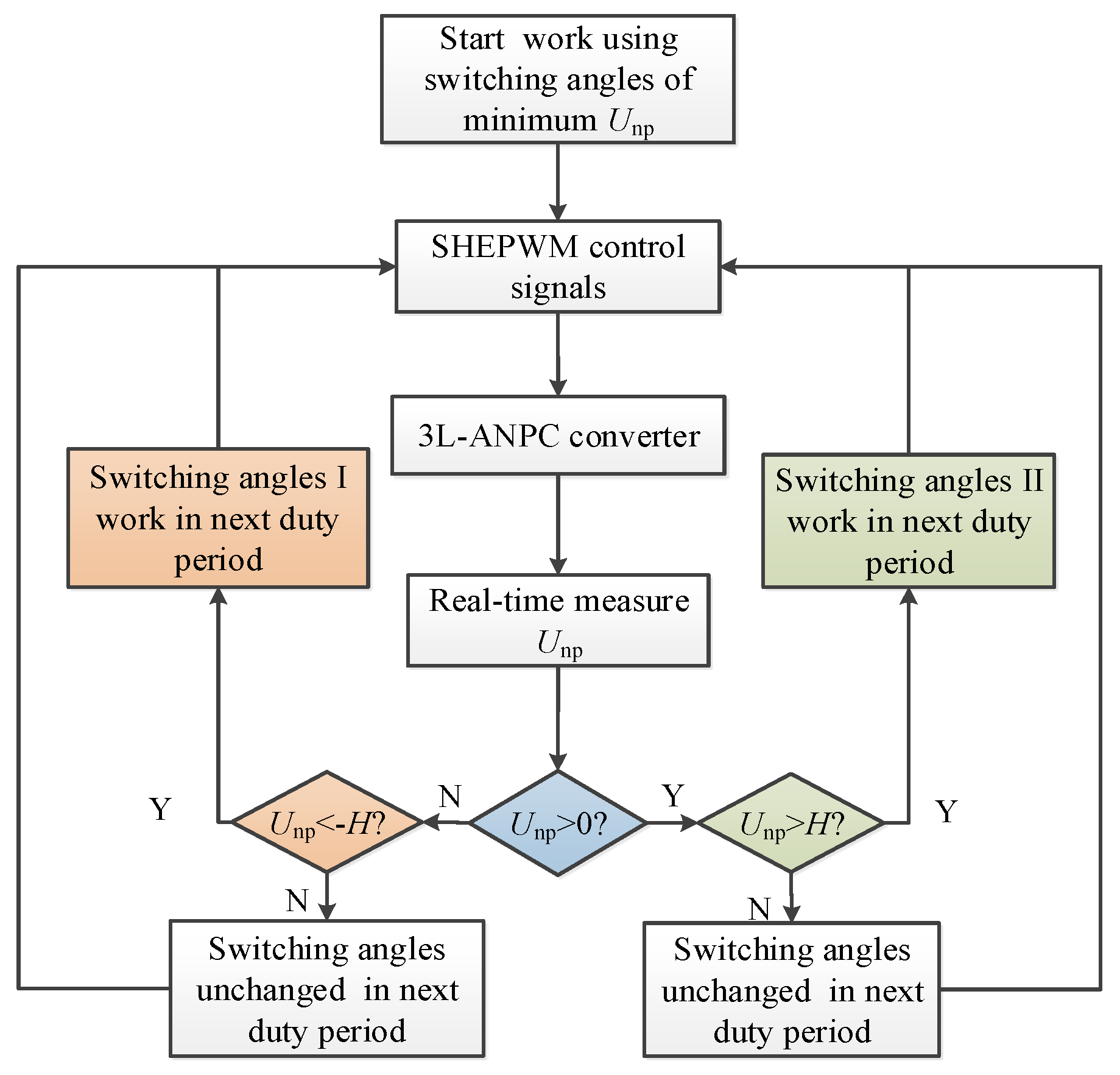
4.2. Voltage Balancing Strategy

If the first set of switching angle I is selected, then the NP will increase, and if the second set of switching angle II is selected, then the NP will decrease. Thus, the NP balancing can be achieved by selecting appropriate SHEPWM switching angles in next fundamental period according to the total offset of the NP in current fundamental period.

Try to avoid the frequent change of switching angle, define H as control factor of the NP. The value of constant H is determined according to the requirement of the NP balancing. Because the amplitude of the NP is generally controlled within 2%–5% of the dc-side voltage, we can take the range of H between 0.5% and 1% of dc-link voltage so that the good performance of the output waveform.

The NP control strategy depends on the polarity of the output currents and the voltage across the lower dc-link capacitor. The block diagram of the proposed control strategy is shown in Figure 6. In the first fundamental period, the switching angles with the minimum |U_np| can be selected and then the NP is measured in real time. U_np is determined by the discrepancy between the reference voltage U_dc,ref which is half of the dc-link voltage, and the lower dc-link capacitor U_C2.

The control strategy of the NP balancing is shown as below.

(1)

When U_np < −H: Select the switching angles I as SHEPWM switching angles in next fundamental period $\Delta Uc<-H$.

(2)

When U_np > H: Select the switching angles II as SHEPWM switching angles in next fundamental period.

(3)

When |U_np| < H: Switching angles unchanged in next duty period.

5. Simulation and Experiment

In this part, the simulation results and experimental results are introduced successively. The feasibility and superiority of the proposed neutral point voltage balancing strategy are verified.

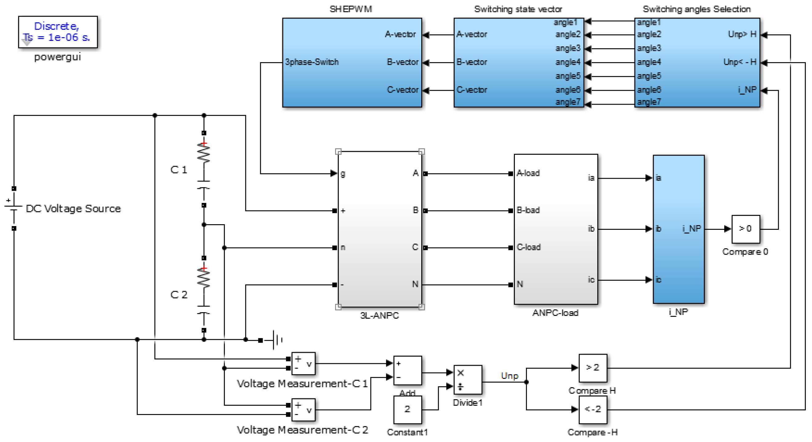
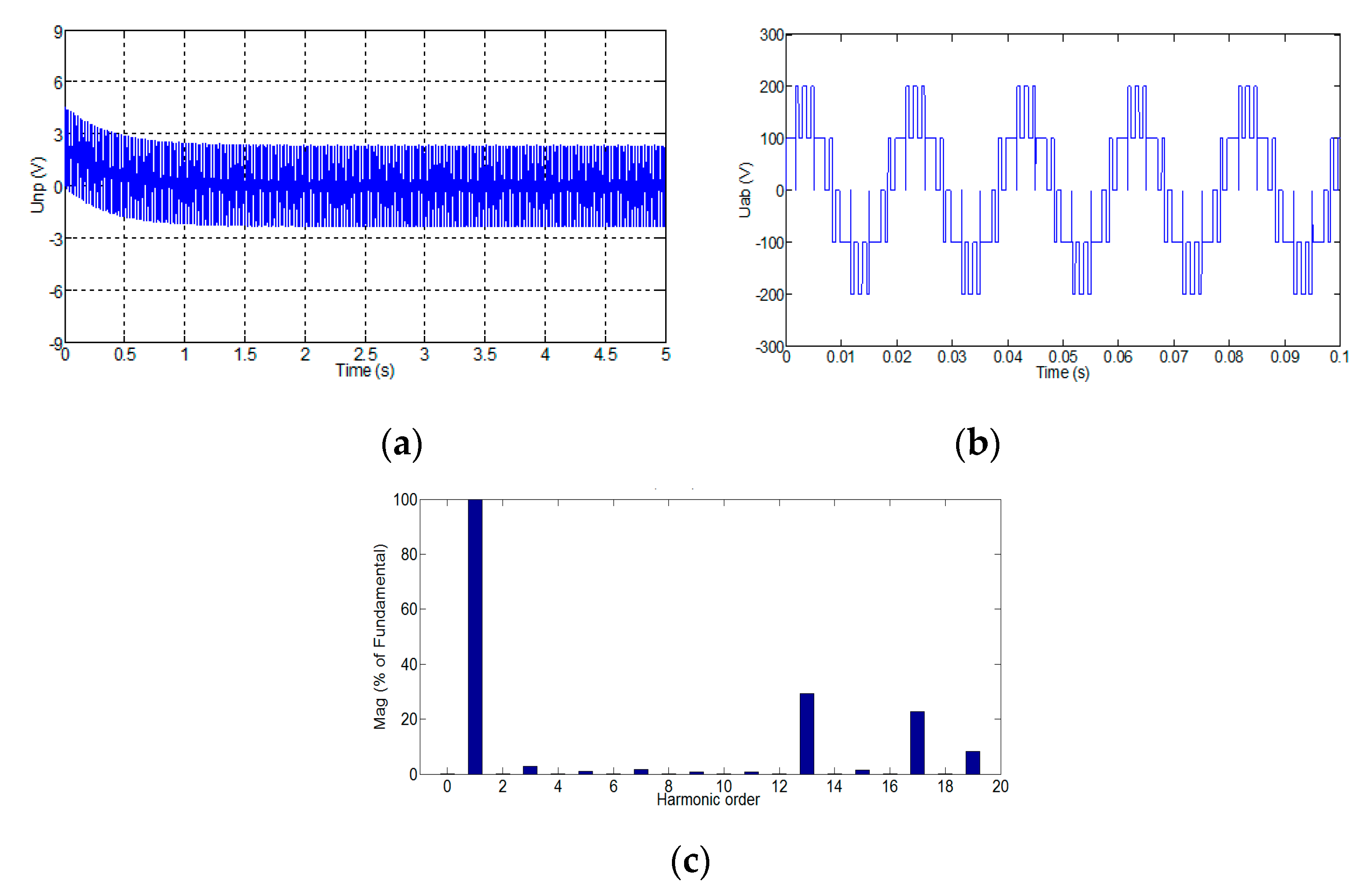
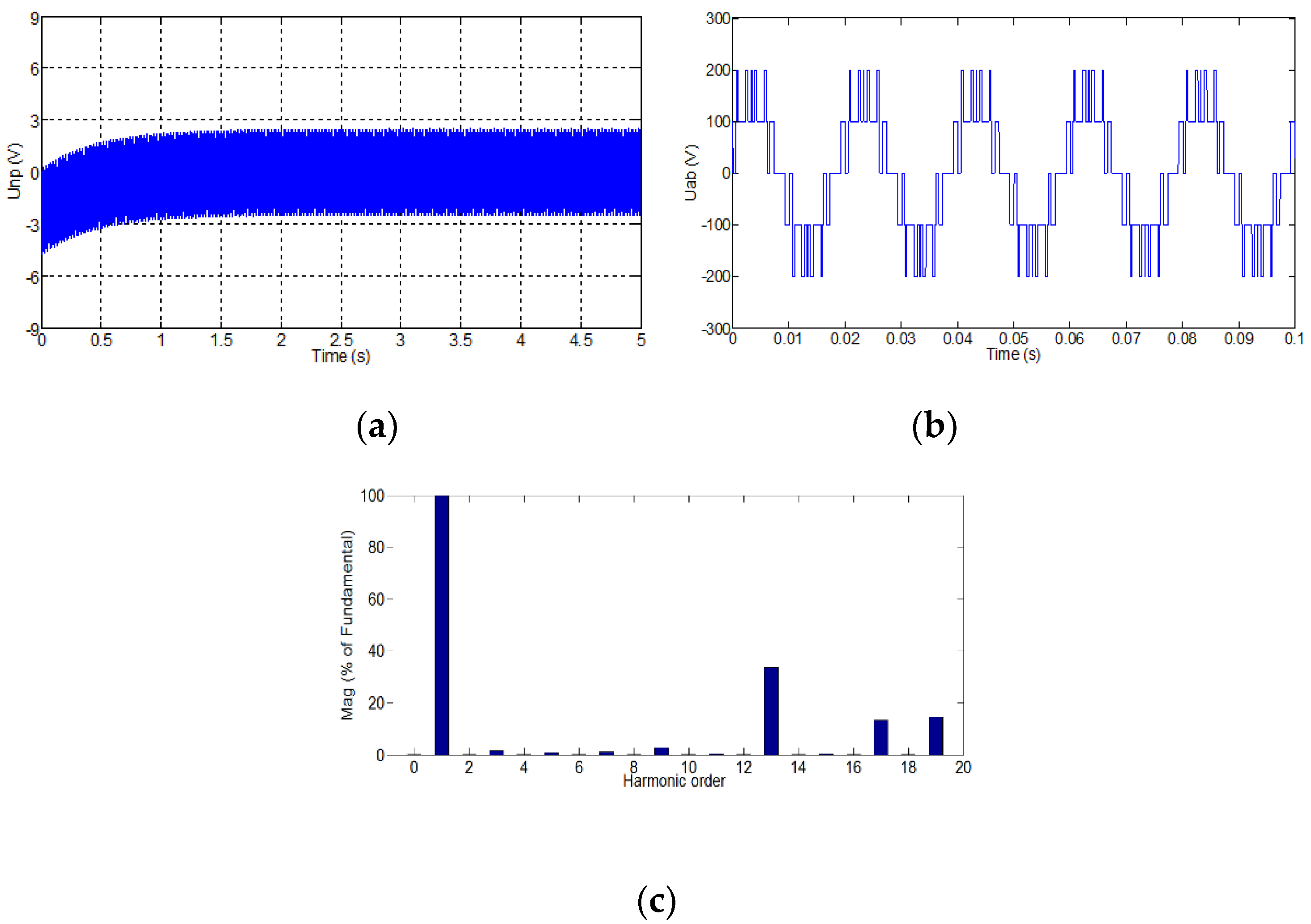
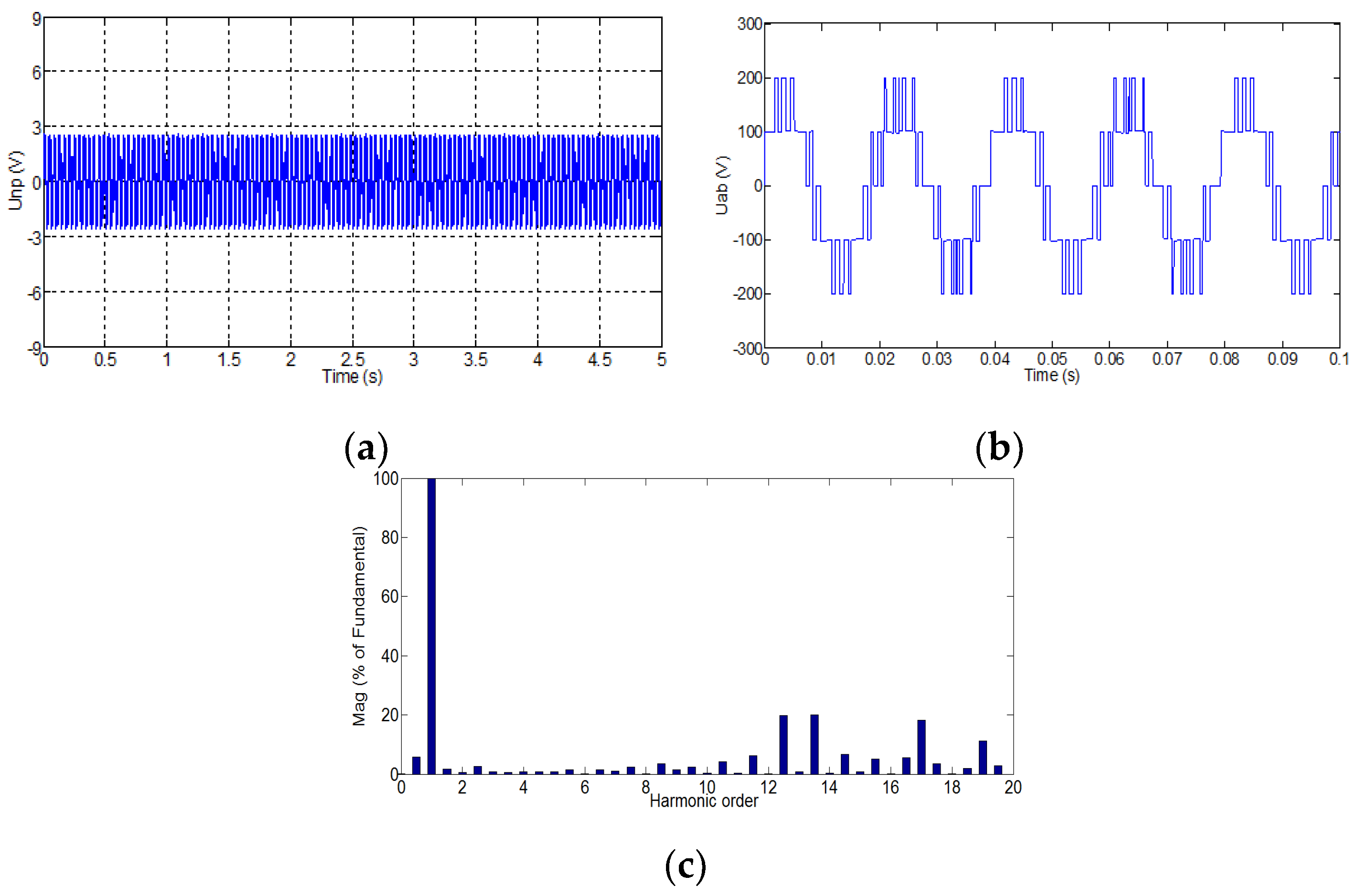
5.1. Simulation Results

First of all, a preliminary simulation is carried out to verify whether this method can achieve neutral point voltage balance on the basis of eliminating specific harmonics compared with the traditional SHEPWM. The parameters of simulation are U_dc = 200 V, C1 = C2 = 4700 μF, R-load = 33 Ω, L-load = 4 mH, and H = 1%, the fundamental frequency = 50 Hz. The simulation model platform of the 3L-ANPC converter was built in MATLAB (2016a)/Simulink using simscape toolbox. Figure 7 shows the screenshot of the scheme implemented in Simulink for such simulations.

Take eliminate the 5th, 7th, 11th, 13th, 17th, and 19th harmonics as an example, and the modulation index is 0.8. When using the first switching angles, Figure 8 shows the simulation results. The NP waveform is shown in Figure 8a. At the beginning stage, the NP is high, and the time constant associated with balancing C₁ and C₂ voltage is approximately 2 s. Figure 8b shows the line voltage waveform. Figure 8c shows the spectrum of line voltage, the 5th, 7th, and 11th order harmonics are eliminated.

Figure 9 shows the simulation result using the second switch angle. The NP waveform is shown in Figure 9a. At the beginning stage, the NP is low, and the time constant associated with balancing C₁ and C₂ voltage is approximately 2.5 s. Figure 9b shows the line voltage waveform. Figure 9c shows the spectrum of line voltage. It can be seen that the 5th, 7th, 11th order harmonics are eliminated.

When using the proposed control strategy, the simulation result is shown in Figure 10. Figure 10a shows the uniform distribution around zero-level of the NP which reach the steady state very quickly. The time constant associated with balancing C₁ and C₂ voltage is very small. Figure 10b shows the line voltage waveform. Figure 10c shows the spectrum of line voltages, where the 5th, 7th, and 11th order harmonics are eliminated. As a result, it only requires filtering harmonic components of higher frequency which makes filter design simple.

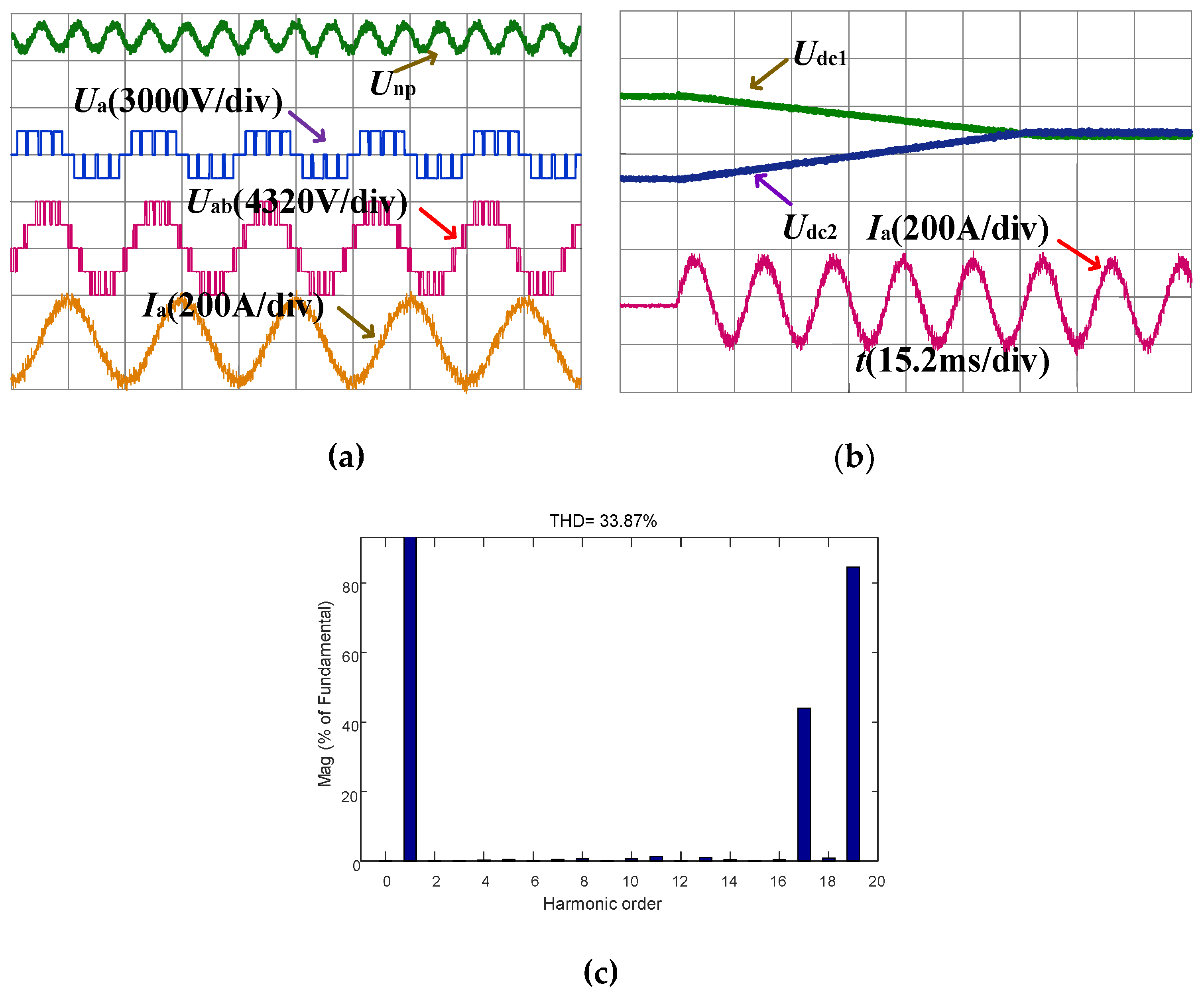
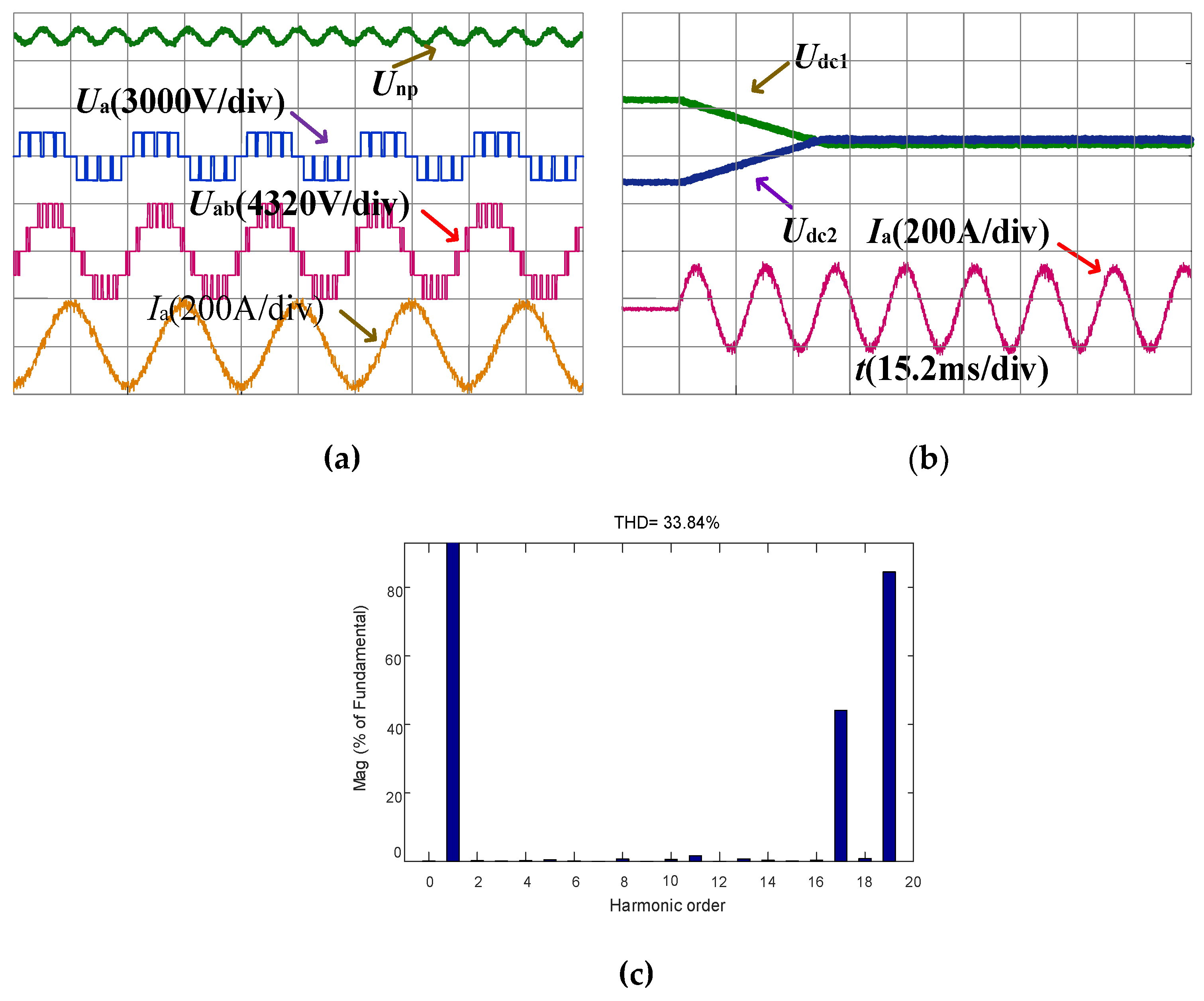
5.2. Experimental Results

The purpose of this experiment is to compare the proposed control strategy with the control strategy in [25]. The experimental platform was implemented with a Texas Instruments TMS320F28335 DSP (Digital Signal Processing) chip, an Altera Cyclone III EP3C55F484C6 FPGA (Field-Programmable Gate Array) chip, and an RT_LAB. The circuit parameters are Udc = 3000 V, C1 = C2 = 3.3 mF, R load = 1 Ω, L load = 80 mH, H = 1%. Figure 11 shows the experimental block diagram.

In order to further verify the effectiveness and superiority of the proposed method, the contrast experiment was made to compare with the neutral point voltage balancing strategy reported in [25]. Figure 12 and Figure 13 show the experimental results of the two strategies under the same experimental environment.

It can be seen from Figure 12a,b and Figure 13a,b, the proposed control strategy takes about 30 ms for capacitor voltage balance, while the control strategy in [25] takes about 90 ms for balance. The proposed control strategy uses a shorter balance time, and the midpoint voltage fluctuation of the proposed control strategy is also smaller. Figure 12c and Figure 13c show that the THD of the two control strategies is almost the same, both of which are about 33.8%.

In conclusion, the proposed control strategy has shorter balancing time and smaller fluctuation of the midpoint voltage.

6. Conclusions

This paper presents an NP balance control strategy for the 3L-ANPC converter based on SHEPWM. In this strategy, the chaotic ACA is used to solve the SHEPWM nonlinear equations. This method does not need initial values of solutions and can get many different solutions in the same modulation index. The effect of different solutions on the NP is different. Some solutions make the NP up, and others make the NP down. Therefore, the NP balancing can be effectively controlled by choosing appropriate solutions. The effectiveness of the proposed control method in the 3L-ANPC converter is verified by the simulation and experiment results.

Although ACA can effectively avoid presetting the initial values of solutions, it will take a long time for ACA to solve equations, so it cannot be achieved the on-line calculation in DSP, the solution of the equation is still need to be pre-calculated, which also determines that this theory can be applied to more level and other topology converters.

References

1. Nabae, A.; Takahashi, I.; Akagi, H. A new neutral-point-clamped PWM inverter. IEEE Trans. Ind. Appl. 1981, 17, 518–523. [Google Scholar] [CrossRef]
2. Bruckner, T.; Bernet, S.; Steimer, P. Feedforward loss control of 3L active NPC converters. IEEE Trans. Ind. Appl. 2007, 43, 1588–1596. [Google Scholar] [CrossRef]
3. Sayago, J.A.; Bruckner, T.; Bernet, S. Comparison of medium voltage IGBT-based 3L-ANPC-VSCs. In Proceedings of the IEEE PESC, Rhodes, Greece, 15–19 June 2008; pp. 851–858. [Google Scholar]
4. Ogasawara, S.; Akagi, H. Analysis of variation of neutral point potential in neutral point clamped voltage source PWM inverters. In Proceedings of the Conference Record of the 1993 IEEE Industry Applications Conference Twenty-Eighth IAS Annual Meeting, Toronto, ON, Canada, 2–8 October 1993; pp. 965–970. [Google Scholar]
5. Yazdani, A.; Iravani, R. A generalized state-space averaged model of the 3L NPC converter for systematic dc-voltage-balancer and current-controller design. IEEE Trans. Power Deliv. 2005, 20, 1105–1114. [Google Scholar] [CrossRef]
6. Maheshwari, R.; Munk-Nielsen, S.; Busquets-Monge, S. Design of Neutral-Point Voltage Controller of a 3L NPC Inverter with Small DC-Link Capacitors. IEEE Trans. Ind. Electron. 2013, 60, 1861–1871. [Google Scholar] [CrossRef]
7. Hornik, T.; Zhong, Q. Parallel PI Voltage–H-infinity Current Controller for the Neutral Point of a Three-Phase Inverter. IEEE Trans. Ind. Electron. 2013, 60, 1335–1343. [Google Scholar] [CrossRef]
8. Yamanaka, K.; Hava, A.M.; Kirino, H.; Tanaka, Y.; Koga, N.; Kume, T. A novel neutral point potential stabilization technique using the information of output current polarities and voltage vector. IEEE Trans. Ind. Appl. 2002, 38, 1572–1580. [Google Scholar] [CrossRef]
9. Zhang, Y.; Li, J. A Method for the Suppression of Fluctuations in the Neutral-Point Potential of a Three-Level NPC Inverter with a Capacitor-Voltage Loop. IEEE Trans. Power Electron. 2017, 32, 825–836. [Google Scholar] [CrossRef]
10. Wu, F.; Feng, F.; Duan, J.; Sun, B. Zero Crossing Disturbance Elimination and Spectrum Analysis of Single-Carrier Seven Level SPWM. IEEE Trans. Ind. Electron. 2015, 62, 982–990. [Google Scholar] [CrossRef]
11. Xiang, C.; Shu, C. Improved Virtual Space Vector Modulation for Three-Level Neutral-Point-Clamped Converter with Feedback of Neutral-Point Voltage. IEEE Trans. Power Electron. 2018, 33, 5452–5464. [Google Scholar] [CrossRef]
12. Wu, X.; Tan, G. Virtual-Space-Vector PWM for a Three-Level Neutral-Point-Clamped Inverter with Unbalanced DC-Links. IEEE Trans. Power Electron. 2018, 33, 2630–2642. [Google Scholar] [CrossRef]
13. Hu, C.; Yu, X. An Improved Virtual Space Vector Modulation Scheme for Three-Level Active Neutral-Point-Clamped Inverter. IEEE Trans. Power Electron. 2017, 32, 7419–7434. [Google Scholar] [CrossRef]
14. Monge, S.B.; Somavilla, S.; Bordonau, J.; Boroyevich, D. Capacitor voltage balance for the neutral-point-clamped converter using the virtual space vector concept with optimized spectral performance. IEEE Trans. Power Electron. 2007, 22, 1128–1135. [Google Scholar] [CrossRef]
15. Du Toit Mouton, H. Natural Balancing of 3L Neutral-Point-Clamped PWM Inverters. IEEE Trans. Ind. Electron. 2002, 49, 1017–1025. [Google Scholar] [CrossRef]
16. Memon, M.A.; Mekhilef, S.; Mubin, M. Selective harmonic elimination in multilevel inverter using hybrid APSO algorithm. IET Power Electron. 2018, 11, 1673–1680. [Google Scholar] [CrossRef]
17. Memon, M.A.; Mekhilef, S.; Mubin, M.; Aamir, M. Selective harmonic elimination in inverters using bio-inspired intelligent algorithms for renewable energy conversion applications: A review. Renew. Sust. Energy 2018, 82, 2235–2253. [Google Scholar] [CrossRef]
18. Yang, K.; Feng, M.; Wang, Y.; Lan, X.; Wang, J.; Zhu, D.; Yu, W. Real-Time Switching Angle Computation for Selective Harmonic Control. IEEE Trans. Power Electron. 2019, 34, 8201–8212. [Google Scholar] [CrossRef]
19. Haghdar, K. Optimal DC Source Influence on Selective Harmonic Elimination in Multilevel Inverters Using Teaching-Learning Based Optimization. IEEE Trans. Ind. Electron. 2019, 67, 942–949. [Google Scholar] [CrossRef]
20. Colorni, A.; Dorigo, M.; Maniezzo, V. Distributed optimization by ant colonies. In Proceedings of the First European Conference on Artificial Life; Elsevier Science Publisher: Amsterdam, The Netherlands, 1992; pp. 134–142. [Google Scholar]
21. Oshaba1, A.S.; Ali, E.S.; Abd Elazim, S.M. Speed control of SRM supplied by photovoltaic system via ant colony optimization algorithm. Neural Comput. Appl. 2017, 28, 365–374. [Google Scholar] [CrossRef]
22. Han, Y.; Shi, P. An improved ant colony algorithm for fuzzy clustering in image segmentation. Neurocomputing 2007, 70, 665–671. [Google Scholar] [CrossRef]
23. Hu, C.; Wang, Q.; Jiang, W.; Chen, Q.; Xia, Q. Optimization Method for Generating SHEPWM Switching Patterns Using Chaotic Ant Colony Algorithm applied to Three-level NPC Inverter. In Proceedings of the 2007 International Conference on Electrical Machines and Systems (ICEMS), Seoul, Korea, 8–11 October 2007; pp. 149–153. [Google Scholar]
24. Li, H.; Wang, S.; Ji, M. An Improved Chaotic Ant Colony Algorithm. Adv. Neural Net. 2012, 7367, 633–640. [Google Scholar]
25. Zhang, X.H.; Yue, W.K. Neutral point potential balance algorithm for three-level NPC inverter based on SHEPWM. Electron. Lett. 2017, 53, 1542–1543. [Google Scholar] [CrossRef]
Figure 1. Simplified circuit diagram of 3L-ANPC converter.
Energies 12 04328 g001
Figure 2. Single phase selective harmonic elimination pulse width modulation (SHEPWM) waveform of 3L-ANPC converter.
Energies 12 04328 g002
Figure 3. Decoding process of the ant colony algorithm.
Energies 12 04328 g003
Figure 4. Two sets of switching angles versus modulation index. (a) Switching angles of the first group (b) Switching angles of the second group.
Energies 12 04328 g004
Figure 5. Three-phase SHEPWM output voltage waveform in 1/4 period.
Energies 12 04328 g005
Figure 6. Block diagram of proposed control strategy.
Energies 12 04328 g006
Figure 7. The screenshot of the simulations in Simulink.
Energies 12 04328 g007
Figure 8. Simulation waveforms when using the first switching angles. (a) The NP waveform. (b) Line voltage waveform. (c) Spectrum of line voltage.
Energies 12 04328 g008
Figure 9. Simulation waveforms when using the second switching angles. (a) The NP waveform. (b) Line voltage waveform. (c) Spectrum of line voltage.
Energies 12 04328 g009
Figure 10. Simulation waveforms when using proposed control strategy. (a) The NP waveform. (b) Line voltage waveform. (c) Spectrum of line voltage.
Energies 12 04328 g010
Figure 11. The block of the experimental details.
Energies 12 04328 g011
Figure 12. Experimental waveforms with proposed control strategy. (a) Midpoint voltage, phase voltage, line voltage and phase current. (b) Upper and lower capacitor voltage, phase current. (c) Spectrum of line voltage.
Energies 12 04328 g012
Figure 13. Experimental waveforms with control strategy in [25]. (a) Midpoint voltage, phase voltage, line voltage, and phase current. (b) Upper and lower capacitor voltage, phase current. (c) Spectrum of line voltage.
Energies 12 04328 g013