Article

Synthesis of Optimal Battery State-of-Charge Trajectory for Blended Regime of Plug-in Hybrid Electric Vehicles in the Presence of Low-Emission Zones and Varying Road Grades

Faculty of Mechanical Engineering and Naval Architecture, University of Zagreb, Zagreb 10002, Croatia
*
Author to whom correspondence should be addressed.
Energies 2019, 12(22), 4296; https://doi.org/10.3390/en12224296
Submission received: 17 October 2019 / Revised: 31 October 2019 / Accepted: 6 November 2019 / Published: 11 November 2019
(This article belongs to the Special Issue PHEVs: Latest Advances and Prospects)

Abstract

:
The powertrain efficiency for plug-in hybrid electric vehicles (PHEV) can be maximized by gradually discharging the battery in a blended regime, where the engine is regularly used all over the driving cycle. A key step in designing an optimal PHEV control strategy for the blended regime corresponds to synthesis of battery state-of-charge (SoC) reference trajectory. The paper first demonstrates that the optimal SoC trajectory can significantly differ from a typical linear-like shape in the case of varying road grade and presence of low-emission zones (LEZ). Next, dynamic programming (DP)-based optimizations of PHEV control variables are conducted for the purpose of extracting and analyzing optimal SoC trajectory patterns. It is shown that the optimality is closely related to the minimization of SoC trajectory length with respect to travelled distance. This finding is used for SoC reference trajectory synthesis in the presence of LEZ and varying road grades. Finally, the overall PHEV control strategy is applied to a PHEV-type city bus and verified by means of computer simulations in comparison with the DP optimization benchmark.

Graphical Abstract

1. Introduction

Plug-in hybrid electric vehicles (PHEVs) offer the functionality of pure electric driving, while successfully tackling the major obstacles related to a wide adoption of battery electric vehicles (BEVs) such as high price, low range, and long charging duration [1]. The PHEV powertrain typically operates in a charge depleting (CD) regime until the battery is discharged to a predefined lower limit value, when the charge sustaining (CS) regime is activated to sustain the battery state-of-charge (SoC) and to extend the driving range. When the driving distance is known in advance, the PHEV battery could be discharged more gradually by regularly using the engine in the so-called blended mode, in order to fully exploit the PHEV powertrain efficiency potential [2]. In this case, the PHEV control strategy becomes more complex and it requires optimal design of battery SoC reference trajectory to be commanded to an explicit or implicit SoC controller. While it is well-known that the optimal SoC trajectory vs. travelled distance is nearly linear for the basic, certification driving cycles, it is clear that it can substantially differ from the linear profile when the low-emission zones (LEZ) [3,4] and varying road grade are considered [5].
Several previous publications have dealt with analyzing optimal battery energy usage throughout the driving cycle under different driving conditions, including varying road grade and LEZ presence [6]. In [7], an energy management strategy relying on driving condition preview is proposed, which generates an explicit trip-specific battery SoC reference based on predicted driving patterns along a trip. An adaptive energy management strategy based on the Pontryagin minimum principle is proposed in [5], which uses predefined maps to adapt control strategy parameters based on driving cycle conditions. An SoC reference generator dealing with varying road grade is presented in [8], which employs a preview of the driving cycle to crudely approximate SoC recharging rates during negative road grades, while using quadratic programming to minimize SoC reference rates during positive road grades to guarantee the final SoC constraint. Reference [9] presents a predefined, heuristically determined rules to modify SoC reference trajectory during steep hill climbing based on velocity and road grade preview. In [3], the CD/CS operation-like SoC reference trajectory generation is proposed for driving cycles including LEZs, where the battery charge is sustained in hybrid driving outside of LEZ, while using pure electric driving within LEZ. Model predictive control (MPC)-based energy management strategies are becoming a research topic of many recent papers, where on-line optimizations of PHEV control variables are performed on a receding horizon [10,11,12]. A Monte Carlo approach is applied in [13] to reconstruct the optimal SoC reference trajectory over an MPC strategy prediction horizon. In [12] and [14], SoC reference is provided to MPC control strategy in the form of terminal condition at the end of MPC optimization time horizon, which is calculated based on real-time traffic flow data in [14], and based on prediction of travelled distance within the following optimization time horizon in [12].
This paper presents a practical method of optimal SoC reference trajectory synthesis for a general case of driving cycles (including the presence of LEZs and varying road grade), which can be applied to any control strategy that requires explicit SoC reference. For verification purposes, the synthesized SoC reference is incorporated into the previously developed PHEV control strategy based on a rule-based controller extended with an equivalent consumption minimization strategy (ECMS) [15]. First, dynamic programming (DP)-based optimizations of control trajectories are conducted for the purpose of obtaining globally optimal SoC trajectories for the given set of driving cycles, and extracting and analyzing their patterns for specific operating conditions. It is shown that the near optimal SoC trajectory can be synthesized as a piecewise linear function of traveled distance, thus leading to a straightforward and computationally efficient synthesis targeted to real-time applications. Finally, the overall control strategy, applied to a PHEV-type city bus, is verified by means of computer simulations, and the results are compared with the DP optimization benchmark.
The main contributions of this paper include: (i) extracting the optimal battery SoC patterns from DP optimization results for different LEZ and varying road grade scenarios, and (ii) proposing a practical, nearly optimal method of optimal SoC reference trajectory synthesis dealing with LEZ and varying road slope scenarios.
The remaining part of the paper is organized as follows. A mathematical model of the PHEV powertrain is described in Section 2. The results of DP optimization of PHEV control variables are presented in Section 3 and the optimal patterns of SoC trajectory are analyzed. The overall PHEV powertrain control strategy, including the SoC reference trajectory synthesis, is described in Section 4. Simulation results and corresponding analyses are presented in Section 5. Concluding remarks are given in Section 6.

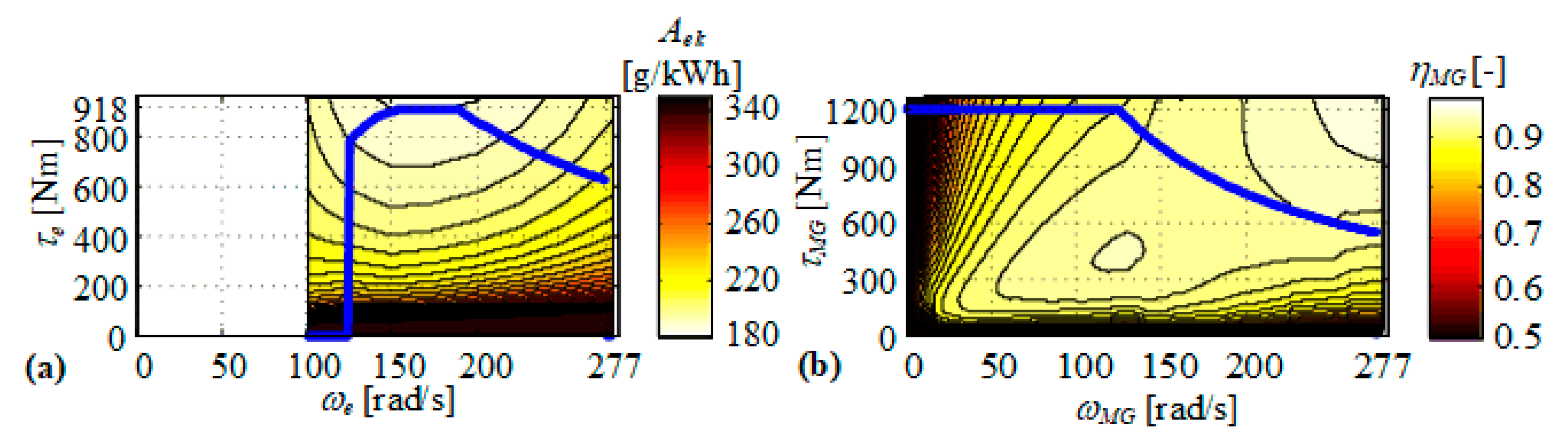
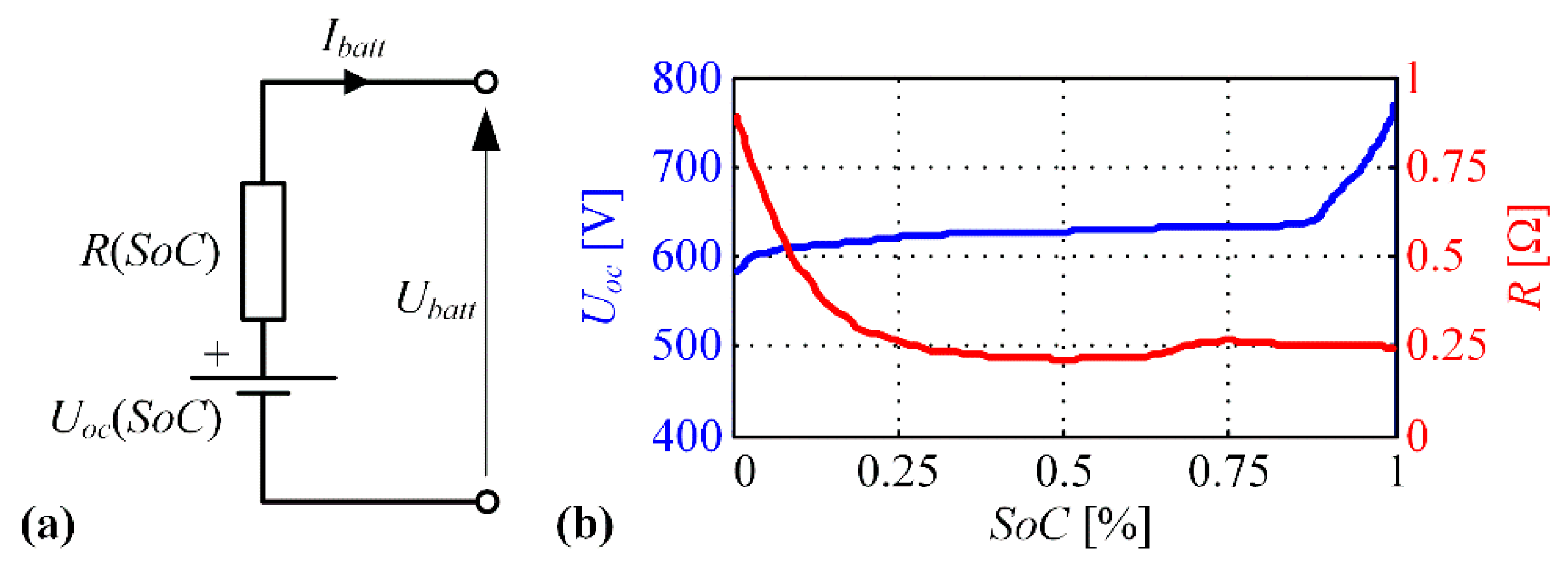
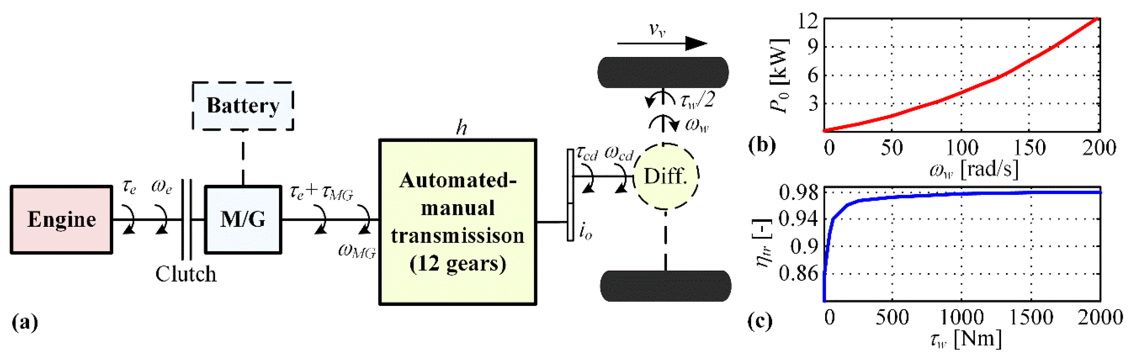
2. Mathematical Model of PHEV Powertrain

The PHEV powertrain configuration considered is of the P2 parallel type, and it includes electric machine operating as motor or generator (M/G machine), internal combustion engine, electrochemical battery, and automated manual transmission with 12 gear ratios (Figure 1). The engine is connected with the rest of powertrain via a clutch, which is disengaged when the engine is switched off in pure electric driving. The PHEV powertrain is modeled in a backward-looking manner [1], resulting in a computationally efficient quasi-static model with only the battery SoC considered as a state variable. The powertrain model elements are parameterized for the case of Volvo 7900 Electric Hybrid city bus [16].
The relations of rotational speeds and torques of different powertrain components are modeled by a set of kinematic equations. The engine rotational speed ω e and M/G machine rotational speed ω M G are related to the vehicle velocity v v and the wheel rotational speed ω w :
ω e = ω M G = i o h ω w = i o h v v r w ,
where i o represents the final drive ratio, h is the transmission gear ratio, and r w is the tire effective radius. The engine torque τ e and M/G machine torque τ M G are combined to deliver the demanded torque at wheels, τ w , and cover the torque/power losses:
τ e + τ M G = τ c d i o h = τ w η t r ( τ w ) + P 0 ( ω w ) ω w i o h ,
where τ c d is the transmission output torque, while η t r ( τ w ) and P 0 ( ω w ) are transmission efficiency and idle power loss maps shown in Figure 1b,c, respectively. These maps have been reconstructed from the data/maps given in [17] and [18] by properly scaling the data with respect to maximum speed and power ratios of the vehicles from [17,18] and the particular PHEV-type bus. The total wheel torque τ w is calculated as [15]:
τ w = r w ( ( M v + m p a s s ) d v v d t + R 0 ( M v + m p a s s ) g cos ( δ r ) F r o l l + ( M v + m p a s s ) g sin ( δ r ) F g r a d e + ρ a i r A f C d v v 2 F a e r o ) ,
where M v and m p a s s represent the empty bus mass and the total mass of passengers, respectively; F r o l l , F g r a d e , F a e r o are rolling, road grade-related and aerodynamic resistances, respectively, where R 0 is the rolling resistance coefficient, ρ a i r is the air density, A f is the bus frontal surface, C d is the aerodynamical drag coefficient, δ r is the road grade, and g is the gravity acceleration (see Appendix A for numerical values of these parameters). The overall power demand P d including the powertrain losses is then calculated as
P d = ω w τ c d = ω w τ w η t r ( τ w ) + P 0 ( ω w ) .
The engine specific fuel consumption A e k and M/G machine efficiency η M G are modeled by maps in dependence of the corresponding rotational speeds and torques (Figure 2). These maps are adopted from the respective maps published in [19] and [20] for similar engine and M/G machine and scaled (based on the Willans line method [21]) with respect to maximum speed and power ratios of the vehicles from [19,20] and the particular PHEV-type bus. The fuel mass flow is calculated from the specific fuel consumption map from Figure 2a (with the unit of A e k converted to g/Ws) by using the following expression
m ˙ f = A e k ( τ e , ω e ) τ e ω e .
The battery is modeled as a charge storage based on the equivalent electric circuit (Figure 3a), where the open-circuit voltage U o c and internal resistance R are set to be dependent on the battery SoC (Figure 3b). The dependences U o c ( S o C ) and R ( S o C ) have been reconstructed from SAFT Ion’Drive 630 V battery system datasheet and available data from [22]. The model is represented by the following state equation [23,24]:
S o C ˙ = U o c 2 ( S o C ) 4 R ( S o C ) P b a t t U o c ( S o C ) 2 Q m a x R ( S o C ) ,
where Q m a x represents the battery total charge capacity with SoC being defined as S o C = Q / Q m a x , while P b a t t represents the battery power which is calculated from the M/G machine power ( P M G ) and efficiency ( η M G , see Figure 2b):
P b a t t =   η M G k τ M G ω M G   P M G .
The exponent k in Equation (7) depends on the M/G machine operating mode: k = 1 for motoring ( P M G > 0 ), and k = 1 for regenerative braking ( P M G < 0 ).

3. Optimization of PHEV Control Variables

This section deals with dynamic programming-based off-line optimization of PHEV powertrain control variables, which is aimed at revealing optimal powertrain behaviors under different driving conditions, and thus providing guidelines for synthesis of optimal SoC reference trajectory and setting a globally optimal benchmark for verification of on-line control strategy.

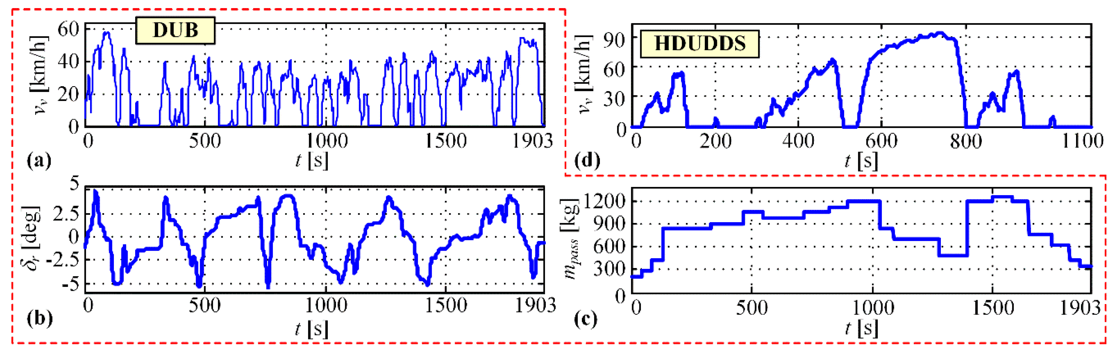
3.1. Considered Driving Cycles and Scenarios

Two driving cycles are used in control variable optimizations and also simulations (Figure 4): (i) realistic city-bus driving cycle recorded in the city of Dubrovnik (designated as DUB cycle), which includes vehicle speed, road grade, and passengers mass time profiles [25]; and (ii) Heavy Duty Urban Dynamometer Driving Schedule driving cycle (HDUDDS), which only includes vehicle speed time profile while assuming zero road grade ( δ r = 0 ) and empty bus ( m p a s s = 0 ). Finally, these driving cycles are replicated several times and concatenated (designated as jxDUB and jxHDUDDS, where j is the number of cycles concatenated), in order to enable discharging of the battery under the blended operating regime.
In order to study the impact of low-emission zones (LEZ) on the optimal PHEV powertrain operation, two hypothetical LEZ sections are introduced in each of the repetitive driving cycles (3xDUB and 3xHDUDDS). The created LEZs are illustrated in Figure 5, where the variable K L E Z takes non-zero values ( K L E Z > 0 ) for LEZ-related road segments, while taking zero value, otherwise.
Apart from LEZ impact on the optimal powertrain operation, the impact of varying road grade is also considered and analyzed. For this purpose, DUB driving cycle is analyzed both for the case of recorded road grade (Figure 4b) and zero road grade. Additionally, three synthetic road grade profiles of different spatial frequencies are generated as
δ r = δ r , m a x sin ( k π s f s ) ,
where δ r , m a x represents the road grade amplitude (here set to 2°), k is the scaling factor determining the spatial frequency, and s f is the total travelled distance (see Figure 6a). These road grade profiles are combined with 4xDUB driving cycle. Figure 6b shows the corresponding altitude profiles. Here, the case of low-frequency road grade, representing long hill climbing followed by long hill descending, can have particularly significant impact on PHEV powertrain operation. Namely, for the optimal operation, the PHEV should apparently discharge the battery in the climbing phase, in order to prepare it for charging during regenerative braking in the descending phase, which would require some kind of predictive control.

3.2. Optimal Problem Formulation

Equation (1) points out that the engine speed ω e and M/G machine speed ω M G are both determined by the vehicle velocity v v via the transmission gear ratio h , where v v is defined by the driving cycle, while h is a control variable to be optimized. The engine torque τ e is chosen as the second control variable to be optimized, where the M/G machine torque τ M G is then determined by Equation (2) to satisfy the demanded torque τ c d . The state, control, and external variables can be written in the vector form as follows:
x = S o C , u = [ τ e   h ] T , v = [ τ w   ω w ] T .
The cumulative fuel consumption is minimized by introducing the following discrete-time cost function:
J = k = 1 N F ( x k ,   u k ,   v k , k ) ,
F ( x k , u k , v k , k ) = m ˙ f , k T d + K L E Z ( k ) m ˙ f , k T d + K g { H ( x k S o C m i n ) + H ( S o C m a x x k ) } + K g { H ( P b a t t m a x P b a t t , k ) + H ( P b a t t , k P b a t t m i n ) } + K g { H ( τ e , k τ e m i n ) + H ( τ e m a x τ e , k ) } + K g { H ( ω e , k ω e m i n ) + H ( ω e m a x ω e , k ) } + K g { H ( τ M G , k τ M G m i n ) + H ( τ M G m a x τ M G , k ) } + K g { H ( ω M G , k ω M G m i n ) + H ( ω M G m a x ω M G , k ) }
where k denotes the discrete time step, T d = 1 s is the discretization time and N is the total number of discrete time steps. The term m ˙ f , k T d corresponds to the current fuel consumption, while the second term K L E Z ( k ) m ˙ f , k T d penalizes the fuel consumption within LEZ by multiplying it with the penalization factor K L E Z shown in Figure 5. Other terms of Equation (11) are introduced to penalize violation of different powertrain constraints. Here, the function H denotes the inverted Heaviside function defined as: H ( z ) = 0 for z ≥ 1, and H ( z ) = 1 , otherwise. The variable K g is weighting factor and it is set to a relatively large value ( K g = 10 12 g) to ensure satisfying the constraints. The state Equation (6) is given in the discrete form as
x k + 1 = f ( x k ,   u k ,   v k ,   k ) , k = 0 , 1 , , N 1 ,
with the initial condition set as x 0 = S o C i , where S o C i is the initial SoC. Finally, the final SoC can be prescribed (to the value S o C f ) by adding the terminal term J f to the cost function given by Equation (10):
min u k ( J f + k = 1 N F ( x k , u k ,   v k , k ) ) ,
J f = K f ( S o C f x N ) 2 = K f ( S o C f f ( x N 1 , u N 1 , v N 1 ) ) 2 ,
where K f is the corresponding weighting factor ( K f = 10 6 g).
The optimization problem formulated by Equations (10)–(14) is solved by dynamic programming (DP) optimization algorithm [26], which can provide globally optimal solution even for nonlinear, nonconvex optimization problems with discretized time, control and state variables. However, the DP algorithm has a high computational complexity which grows exponentially with the number of state and control variables. Having only one state and two control variables in the particular powertrain model (see Equation (9)) makes the DP algorithm viable for PHEV control variables optimization [27].

3.3. Optimization Results

First, DP optimizations have been conducted for the case of zero road grade, initial SoC equal to 90% ( S o C i = 90%) and the target final SoC equal to 30% ( S o C f = 30%). The corresponding optimal SoC trajectories are given in Figure 7 (blue lines) with respect to travelled distance, along with linear trajectories connecting the initial and final SoC points. Evidently, the optimal SoC trajectories are close to the linear ones with almost ideal correlation ( K 1 ; K is obtained by using corrcoef(.) function in Matlab).
Based on the observation that the optimal SoC trajectory has a linear, i.e., shortest length form, it may be hypothesized that the optimality of SoC trajectory is related to its length when expressed with respect to travelled distance. This is further analyzed in Appendix B (for more details see [28]).
Next, DP optimizations have been conducted in the case of LEZ presence and zero road grade. The resulting optimal SoC trajectories are shown in Figure 8 (blue lines), along with the shortest-length (piecewise linear) SoC trajectories respecting the requirement on electric-only driving within LEZs (see the next section for details on synthesizing the shortest-length SoC trajectories). The results are shown for two pairs of initial and final SoC values: (i) S o C i = 90%, S o C f = 30% (Figure 8a,c), and (ii) S o C i = 50%, S o C f = 50% (Figure 8b,d). The obtained optimal SoC trajectories are aligned well with the shortest-length ones, thus confirming the posed hypothesis on the optimality of shortest-length SoC trajectory when considering the presence of LEZs, as well. This is particularly visible in the Case (ii) (Figure 8b,d), where the battery is being recharged prior to reaching a LEZ, thus preparing for discharging while traversing through the LEZ in the electric-only driving mode.
Figure 9 shows the impact of realistic (recorded) road grade on the optimal shape of SoC trajectories for repetitive DUB driving cycles and the cases without and with LEZ presence. Although the optimal SoC trajectories preserve shortest-length (piecewise) linear-like trends, a notable offset- and high-frequency content-related distortion from the shortest-length trajectories is observed (particularly in the case of LEZ presence, Figure 9b,c). Furthermore, Figure 10b,c reveal that the optimal SoC trajectories obtained for sinusoidal road grade profiles (see Figure 6a) strictly decrease when the road grade is positive (uphill driving), while they increase due to the regenerative braking when the road grade is negative (downhill driving). Consequently, the deviation from the linear-like trajectory is most emphasized for the low-frequency road grade profile (Figure 10b). In the case of highest road grade frequency (Figure 10d) the SoC trajectory distortion is significantly smaller and comparable to that obtained by using the recorded road grade profile (Figure 10a). Note that the minimum SoC is exceptionally reduced to 0% in the low-frequency optimization run (Figure 10b), in order to facilitate comparative analysis with other scenarios in the particular case of long uphill driving (see Figure 6b).
The shape of optimal trajectory in Figure 10b suggests that this trajectory may also be represented by a piecewise-linear profile, consisting of at least two sections corresponding to uphill and downhill driving. In order to analyze and potentially exploit this hypothesis, the optimal SoC trajectories from Figure 10 are decomposed and rearranged into battery discharging and charging sections (Figure 11a). Here, predominantly the discharging part is relevant from the standpoint of SoC reference trajectory synthesis, since in the case of battery recharging the battery SoC profile is mostly determined by regenerative braking power determined by the driving cycle and not by the SoC reference trajectory. The SoC trajectory decomposition indeed reveals that the SoC trajectory during discharging now follows shortest-length (linear-like) shape, as in the previous cases (cf. Figure 7 and Figure 8). Based on this observation, the shortest-length SoC trajectory pattern can also be used for SoC reference trajectory synthesis in the case of varying road grade (see next section).
Figure 11b gives the distribution of optimal rate of change of SoC with respect to power demand P d . The clear functional dependence can be observed for the range of negative to mid positive power demands (regenerative braking and electric-only driving, respectively), while there is no clear dependence above ≈70 kW, because both electric and hybrid driving modes are active for these high-power demands (i.e., d S o C / d t can be negative and approximately zero, respectively). The set of points which exhibit clear dependence of SoC rate on power demand are approximated by the 2nd-order polynomial (red dashed line in Figure 11b) for the purpose of SoC reference trajectory synthesis in the next section.

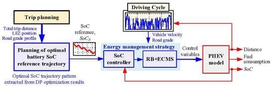
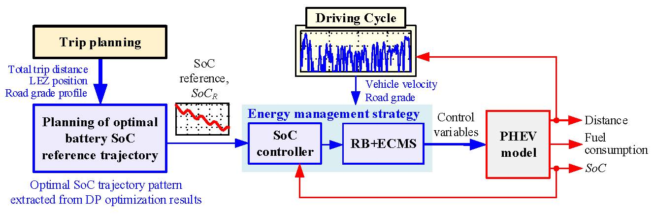
4. PHEV Powertrain Control Strategy

This section first presents the basic control strategy of a PHEV powertrain, which is aimed at selecting proper powertrain operating mode and instantaneously optimizing its operating point (more details can be found in [15]). Next, the design of optimal SoC reference trajectory, fed to the basic control strategy (i.e., its SoC feedback controller), is presented for the cases of LEZ presence and varying road grade.

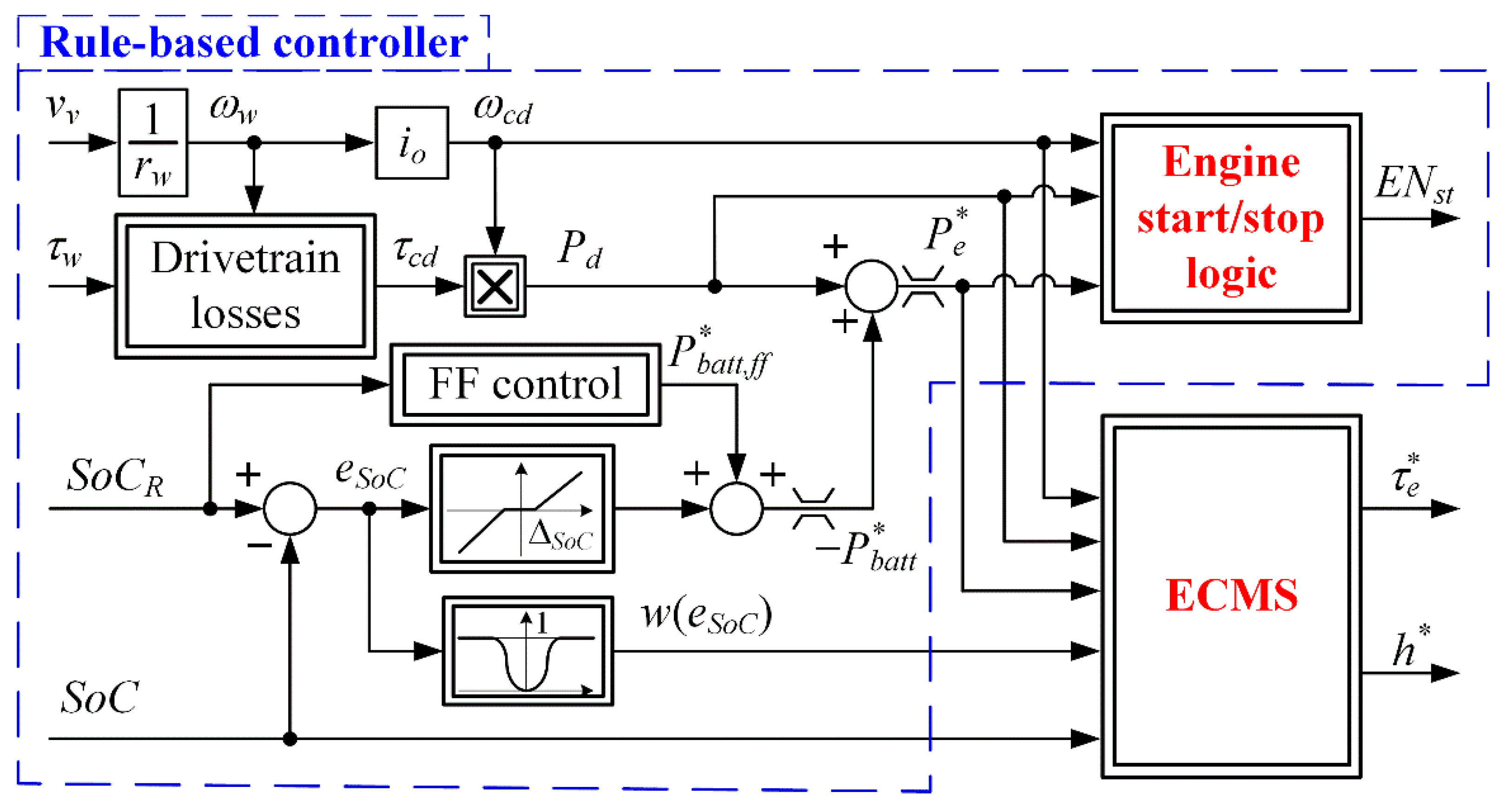
4.1. Basic Control Strategy

The powertrain is controlled by a rule-based (RB) controller combined with instantaneous optimization of the powertrain point (see block diagram in Figure 12 and [24] for the control concept details). The RB controller includes engine start/stop logic which determines whether the electric or hybrid driving mode is activated, and a proportional SoC controller incorporating a dead-zone and extended with feedforward control (the block FF control in Figure 12). The feedforward controller improves tracking of the SoC reference trajectory ( S o C R ). The engine power demand P e * is calculated from the total power demand P d (defined by the vehicle velocity v v and the wheel torque demand τ w , see Equations (1)–(3) and Figure 12) and the SoC controller power demand P b a t t * . The signal P e * is used as an input to the simple engine start/stop logic, which switches the engine on ( E N s t = 1 ) if the engine power P e * is larger than the threshold P o n , while the engine is switched off if P e * is lower than the threshold P o f f < P o n ( E N s t = 0 ). Exceptionally, the engine can be kept switched on in the case P e * < P o f f , when the M/G machine cannot solely satisfy the power demand due to the speed-dependent torque constraint (i.e., τ M G max ( ω M G ) ω M G < P d ; see the blue line in Figure 2b).
The instantaneous optimization is based on the equivalent consumption minimization strategy (ECMS) [29], where the following equivalent fuel consumption m ˙ e q is subject of minimization [24]:
min τ e , h m ˙ e q = { m ˙ f + m ˙ f + A e k η b a t t , c P b a t t A ¯ e k η b a t t , d 1 P b a t t m ˙ b a t t , for   P b a t t   <   0 , for   P b a t t   >   0 .
Here, the term m ˙ f is real fuel mass flow, while the second term ( m ˙ b a t t ) relates to virtual fuel mass flow accounting for the power drawn from or stored in battery ( P b a t t ), where η b a t t , d is battery efficiency during discharging, η b a t t , c is round-trip loss-related efficiency during charging, and A ¯ e k is the mean engine specific fuel consumption during discharging (see [24] and [15] for more details). The ECMS optimization is performed over the transmission gear ratio h and the engine torque τ e (i.e., two degrees of freedom, 2D-ECMS). The iteration through discrete gear ratio values h directly impacts the engine speed ω e (see Equation (1) where v v is set to its current value). In order to ensure SoC sustainability, the engine torque search range is made dependent on the SoC control error e S o C = S o C R S o C (see function w ( e S o C ) in Figure 12, [15]). When the SoC error is zero, the search range is of maximum width, i.e., between the absolute lower limit P o f f / ω e and the absolute upper limit τ e m a x ( ω e ) . For increasing SoC error, the engine torque search range becomes narrower and finally diminishes in the operating point defined by τ e   =   P e * / ω e (i.e., one degree of freedom left, 1D-ECMS), where satisfying the RB controller power demand P e * guarantees the SoC sustainability. The final control strategy is denoted as RB+ECMS.
When the engine is switched off and only the M/G machine is propelling the vehicle, the electricity consumption is minimized (instead of the equivalent fuel) by varying only transmission gear ratio h . Namely, P b a t t / η b a t t , d is minimized in the motoring mode, and η b a t t , c P b a t t is minimized in the generator mode; where η b a t t , d and η b a t t , c denote the corresponding battery discharging and charging efficiencies, respectively.
The mere application of RB+ECMS control can result in frequent switching of gear ratios, thus deteriorating the driving comfort and drivability. Therefore, a gear shift delay (GSD) algorithm is introduced, which is aimed at reducing the number of gear ratio switching events. The ECMS cost function (15) is extended by a discount factor r f , as given by
m ˙ e q = r f ( t s h , h k 1 , h k ) [ m ˙ f + m ˙ b a t t ( P b a t t ,   η b a t t , A e k ) ] .
The discount factor is defined as
r f = { r 0 + t s h 1 r 0 t t h , for   t s h < t t h   and   h k = h k 1 1 , for   t s h t t h   or   h k h k 1 ,
where r 0 = r f ( t s h = 0 ) is the initial/reset value of discount factor (i.e., at the instant of previous, ( k − 1)th gear shift event), t s h is the time elapsed from the previous gear shift event, and t t h is the time threshold in which the discount factor r f reaches the value of 1. The discount of the cost function is provided if the current gear ratio h k is selected to be equal to the previous gear ratio h k 1 , and if the elapsed time from the previous gear shift event is less than the threshold t t h , thus encouraging the ECMS optimization to keep the current gear ratio for somewhat prolonged period, i.e., to avoid frequent switching of gear ratio.

4.2. Synthesis of Optimal SoC Reference Trajectory

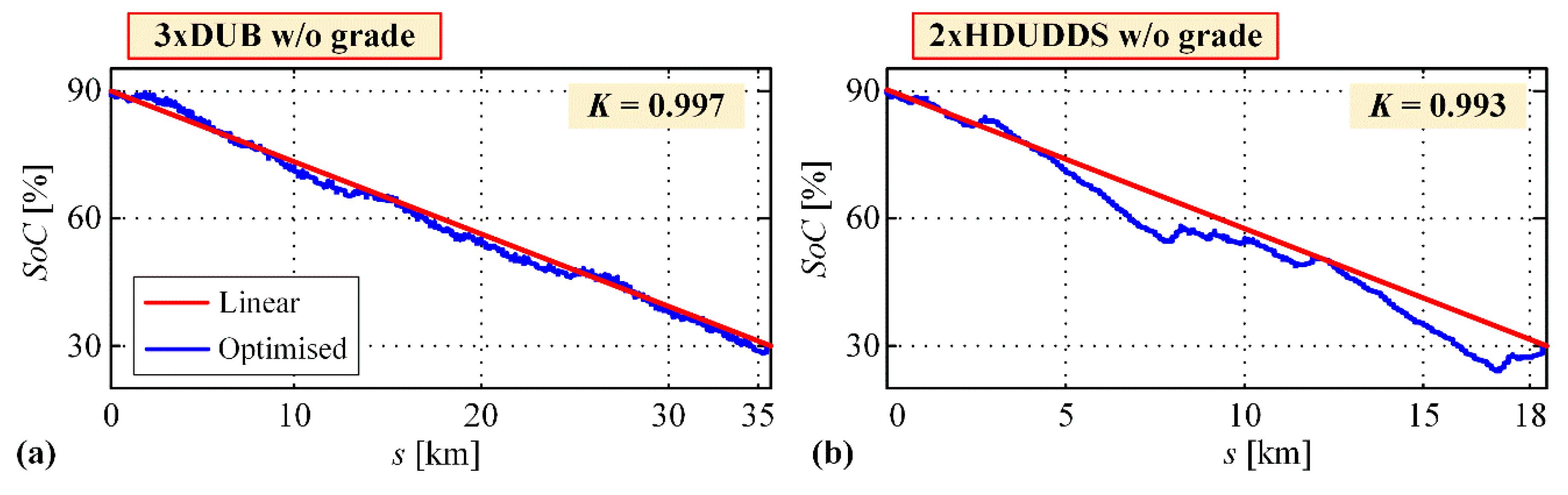
4.2.1. Scenario 1: Zero Road Grade and no LEZ Presence

Based on the principle of designing the shortest-length SoC reference trajectory as the optimal one (Section 3, Appendix B), the following simple-to-implement expression for the SoC reference trajectory applies in the basic scenario with no LEZ presence and zero road grade (see red line in Figure 7):
S o C R ( s ) = S o C R ( 0 ) + s S o C R ( s f ) S o C R ( 0 ) s f ,
where s f is the total travelled distance.

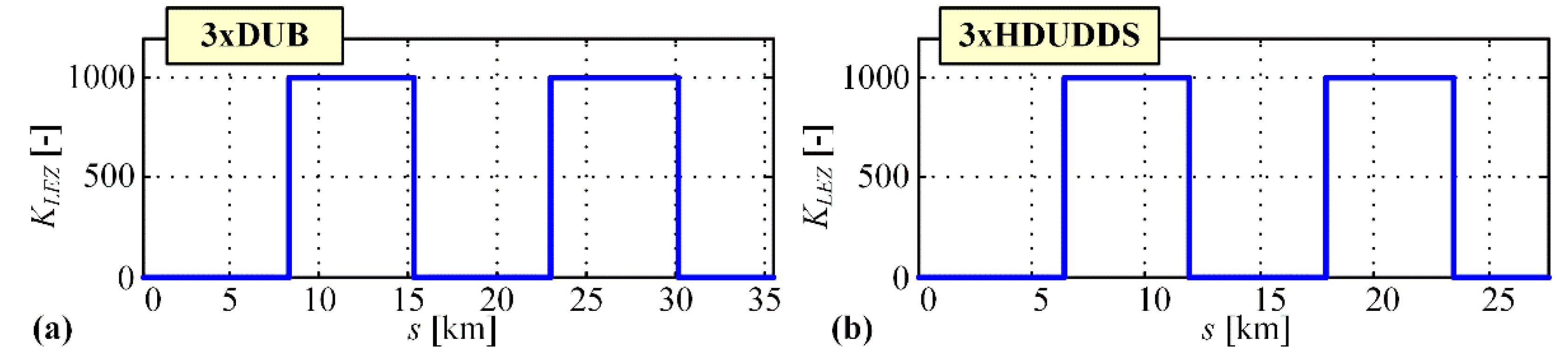
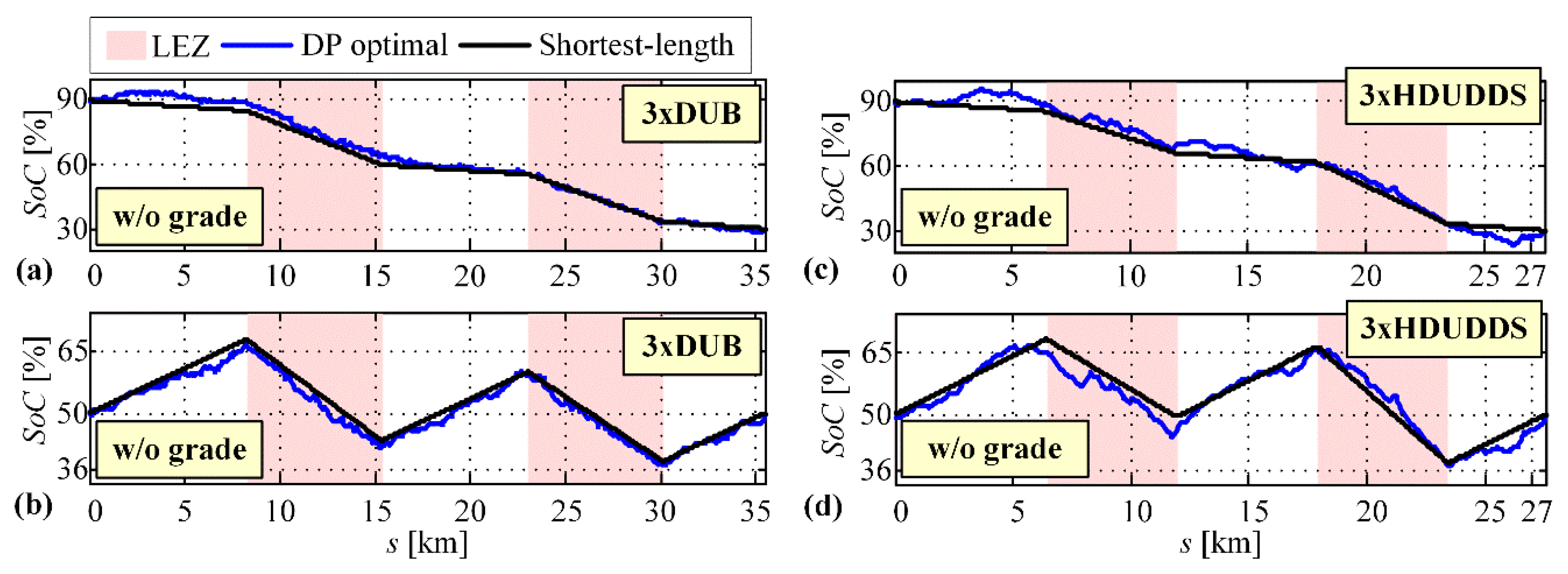
4.2.2. Scenario 2: Zero Road Grade and LEZ Presence

The same principle of designing the shortest-length SoC trajectory is also applied in the case of LEZ presence, where the requirement related to pure electric driving within LEZs is respected. The following expression for the SoC trajectory length can be derived [4]:
L ( s ) = r = 1 N r Δ s r 1 + ( Δ S o C r Δ s r ) 2 + l = 1 N l Δ s l 1 + ( Δ S o C l Δ s l ) 2 ,
where the route is divided into segments, and N r and N l are the total number of these segments outside and within LEZ, respectively, and the terms Δ S o C r / Δ s r = ( S o C r S o C r 1 ) / ( s r s r 1 ) and Δ S o C l / Δ s l = ( S o C l S o C l 1 ) / ( s l s l 1 ) denote the SoC depletion gradients for each segment. Since pure electric driving is preferred within LEZs (the engine is activated only when the M/G machine cannot satisfy the power demand), the LEZ-related SoC depletion gradient is predominantly dependent on the road power demand. Therefore, only the SoC depletion gradients occurring outside the LEZ can be regulated by the control strategy, and they are used for the minimization of overall SoC trajectory length:
min L ( s ) =   min Δ S o C r Δ s r r = 1 N r Δ s r 1 + ( Δ S o C r Δ s r ) 2 .
Due to the convexity of function under sum, the minimum of Equation (20) is achieved for a constant value of SoC depletion gradient Δ S o C r / Δ s r over all-time steps r , thus resulting in a piecewise linear shape of overall SoC trajectory (see [4] where the same principle is used for the calculation of SoC trajectory which minimizes battery losses). The optimal SoC depletion gradient can, thus, be calculated as
Δ S o C r Δ s r =   S o C f S o C i Δ S o C L E Z , Σ r = 1 N r Δ s r ,
while considering the predefined initial and final SoC values S o C i and S o C f , respectively, and denoting the total SoC depletion within all LEZ segments as Δ S o C L E Z , Σ =   l = 1 N l Δ S o C l (assumed to be known in advance). The denominator r = 1 N r Δ s r represent the total travelled distance outside of LEZs. The shortest-length trajectories calculated by Equation (21) are shown by black lines in Figure 8 and Figure 9, where the total LEZ-wise SoC depletion Δ S o C L E Z , Σ , is taken from the DP optimization results. This SoC depletion is not known in advance and should be properly estimated in applications. In the next section, robustness of the synthesis method is tested with respect to errors of estimation of Δ S o C L E Z , Σ .

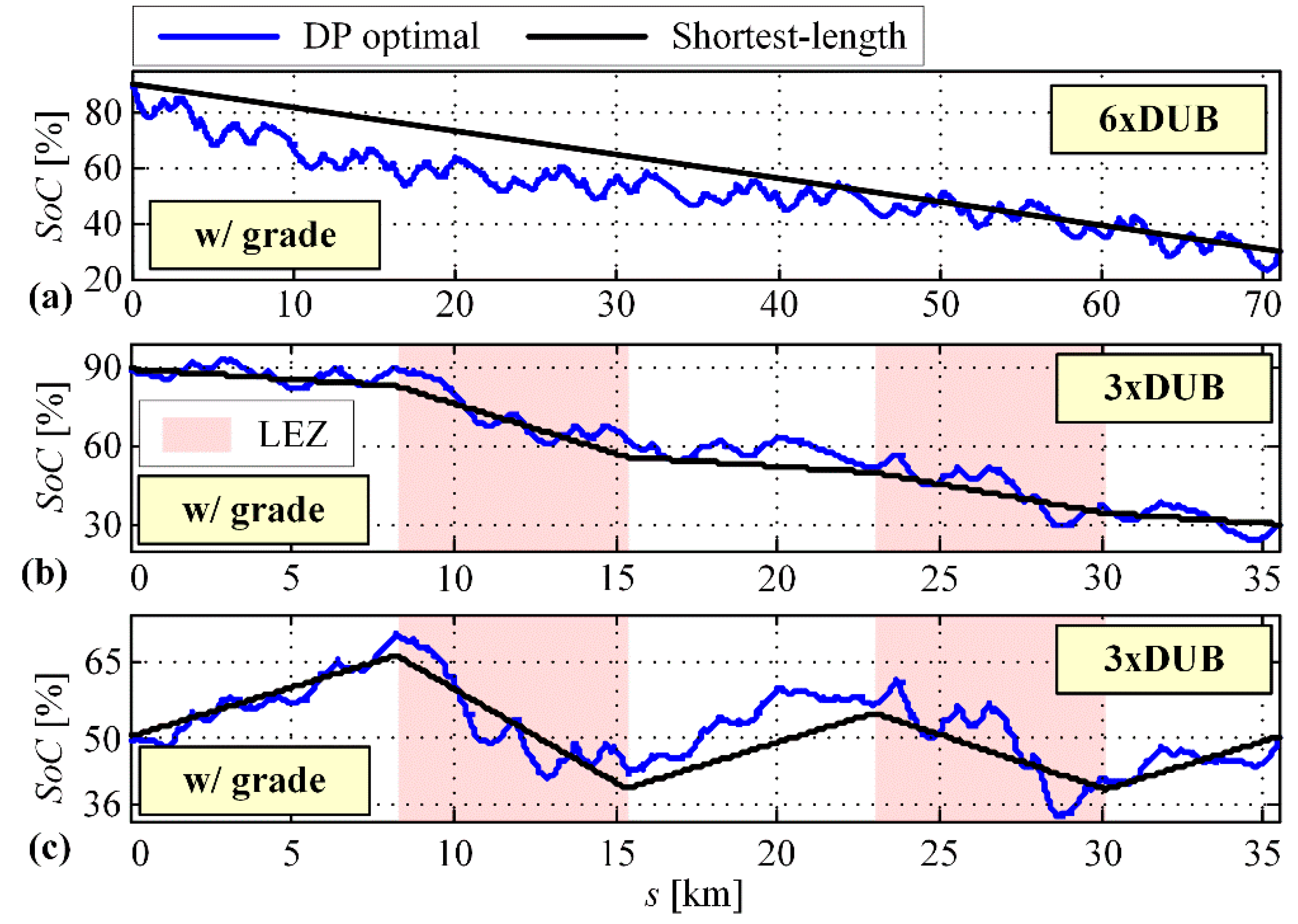
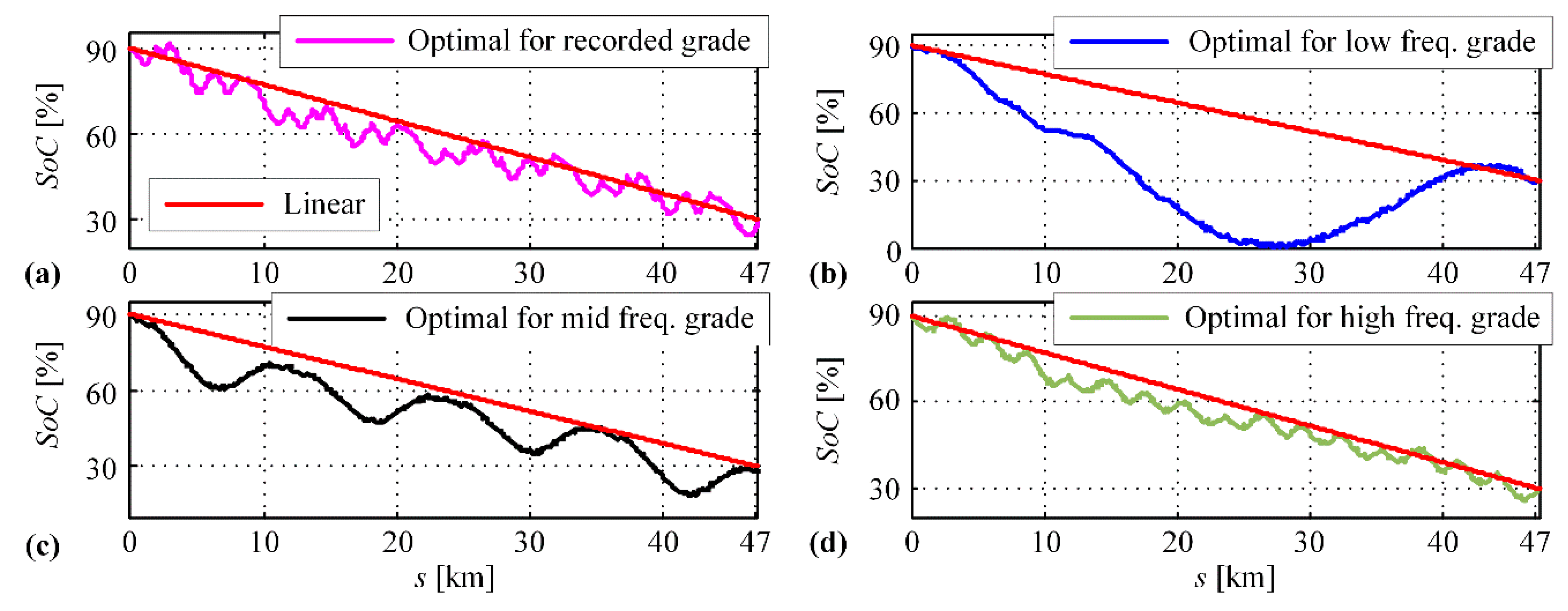
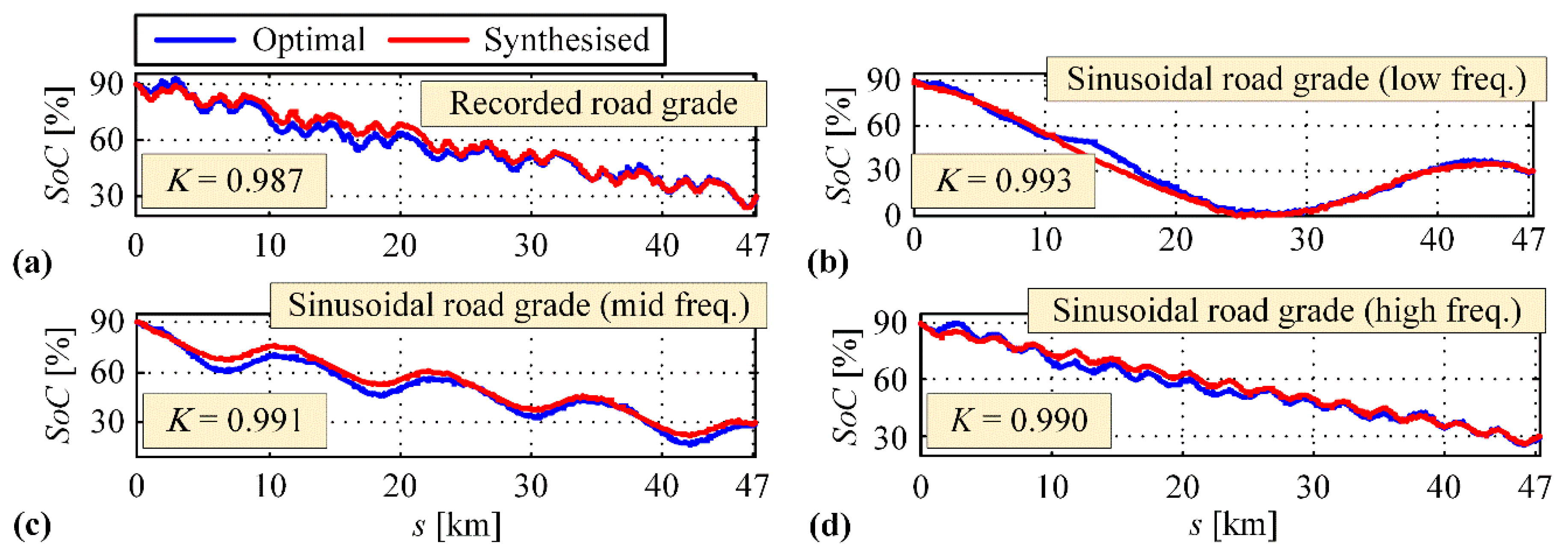
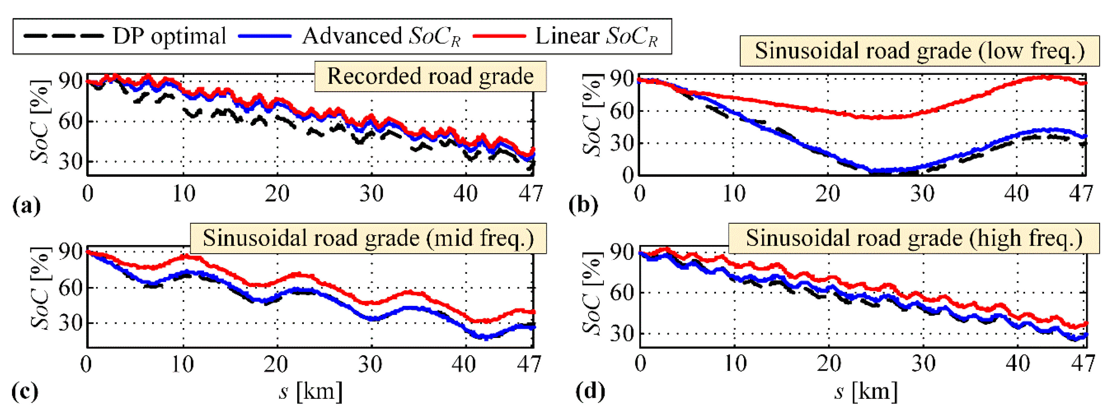
4.2.3. Scenario 3: Variable Road Grade and no LEZ Presence

In the case of varying road grade, the synthesis of SoC reference trajectory is based on the 2nd-order polynomial fitting of d S o C / d t vs. P d curve given in Figure 11b (red dashed line), and the assumption that the power demand profile P d and the vehicle velocity v v are known in advance (or properly estimated). The SoC gradient in pure electric driving for all time steps is, thus, calculated as
Δ S o C R , i + Δ s i =   ( k 1 P d , i 2 + k 2 P d , i + k 3 ) S o C ˙ a p p Δ t Δ s i = ( k 1 P d , i 2 + k 2 P d , i + k 3 ) S o C ˙ a p p 1 v v , i , for   P d , i P d , t h ,
where the term S o C ˙ a p p represents the 2nd-order polynomial fitting curve from Figure 11b, Δ s i is the travelled distance within ith time step, and P d , t h > 0 is the power demand threshold obtained in an iterative manner starting with the initial value conservatively set to P d , t h = 0 . The gradient Δ S o C R , i + / Δ s i is limited with respect to SoC rate lower and upper limit values given in Eq. (23), which are obtained by feeding the maximum discharging (i.e., negative) and maximum charging (i.e., positive) battery power into the battery state Equation (6).
1 v v , i S o C ˙ m i n Δ S o C R , i + Δ s i 1 v v , i S o C ˙ m a x .
As in the case of LEZ, where the SoC trajectory is divided into segments occurring outside and inside LEZ, the SoC trajectory is divided here into hybrid and pure electric driving parts as:
j = 1 N j Δ S o C R , j Δ s j Δ s j Hybrid   driving +   i = 1 N i Δ S o C R , i + Δ s i Δ s i Pure   electric   driving = S o C f S o C i ,
where N j is the total number of time steps for which the condition P d , t h < P d , k P d m a x is satisfied (with P d m a x denoting the highest power demand value), while N i is the total number of steps for which the condition P d , k P d , t h is satisfied. Since the SoC gradient in the pure electric driving segments is defined by Equation (22), it remains to determine the SoC gradients in the hybrid driving mode ( P d , i > P d , t h , for all time steps i). According to the optimal discharging curves shown in left-hand side of Figure 11a, the optimal SoC trajectories for different road grade profiles have linear-like shape and thus nearly shortest length. Similarly as in the case of LEZ presence, the SoC trajectory of shortest length can be achieved by applying a constant SoC gradient value in all hybrid driving time instants. Based on Equation (24), the constant discharging SoC gradient, which satisfies the initial and final SoC values and accounts for the total SoC depletion in the pure electric driving, can be calculated as
Δ S o C R Δ s = S o C f S o C i i = 1 N i Δ S o C R , i + Δ s i Δ s i j = 1 N j Δ s j .
This SoC gradient is further limited to ensure its feasibility:
1 v v , j S o C ˙ a p p ( P d , j ) Δ S o C R Δ s 1 v v , j S o C ˙ m a x , j [ 1 ,   N j ] ,
where the lower limit is imposed because it is not feasible to have the SoC gradient in hybrid driving lower (i.e., larger in absolute value) than that in the pure electric driving (here approximated by S o C ˙ a p p ( P d , j ) , see Equation (22)), while the upper limit is again imposed to reflect the maximum battery power. The feasibility condition (26) greatly depends on the power threshold P d , t h , which is initially set to zero. If the constant SoC rate Δ S o C R / Δ s obtained by the guessed threshold value P d , t h does not respect constraint from Equation (26), the threshold P d , t h is incrementally increased by 10 kW step size until the respective SoC rate Δ S o C R / Δ s becomes feasible.
Referring to the results shown in Figure 13, the SoC trajectories synthesized according to the above procedure closely follow the optimal SoC trajectories. This is quantitatively confirmed by means of correlation index values K given in Figure 13, which closely approach the ideal-correlation value of 1 (cf. Figure 7).
It should be noted that this synthesis procedure is not directly applicable in most applications, because the required future power demand profile and vehicle velocity are usually not available. However, there is a good potential for application to vehicles driving on predetermined and fixed routes, such as buses and delivery vehicles typically equipped with GPS/GPRS-based tracking devices, where the upcoming power demand profiles can be effectively predicted based on historical data [30]. Also, this method could be applied to personal vehicles by using the data provided by the GPS-based navigation service, including an option of sharing the traffic data between the vehicles, similarly as it is done within the PHEV energy management approach described in [14].

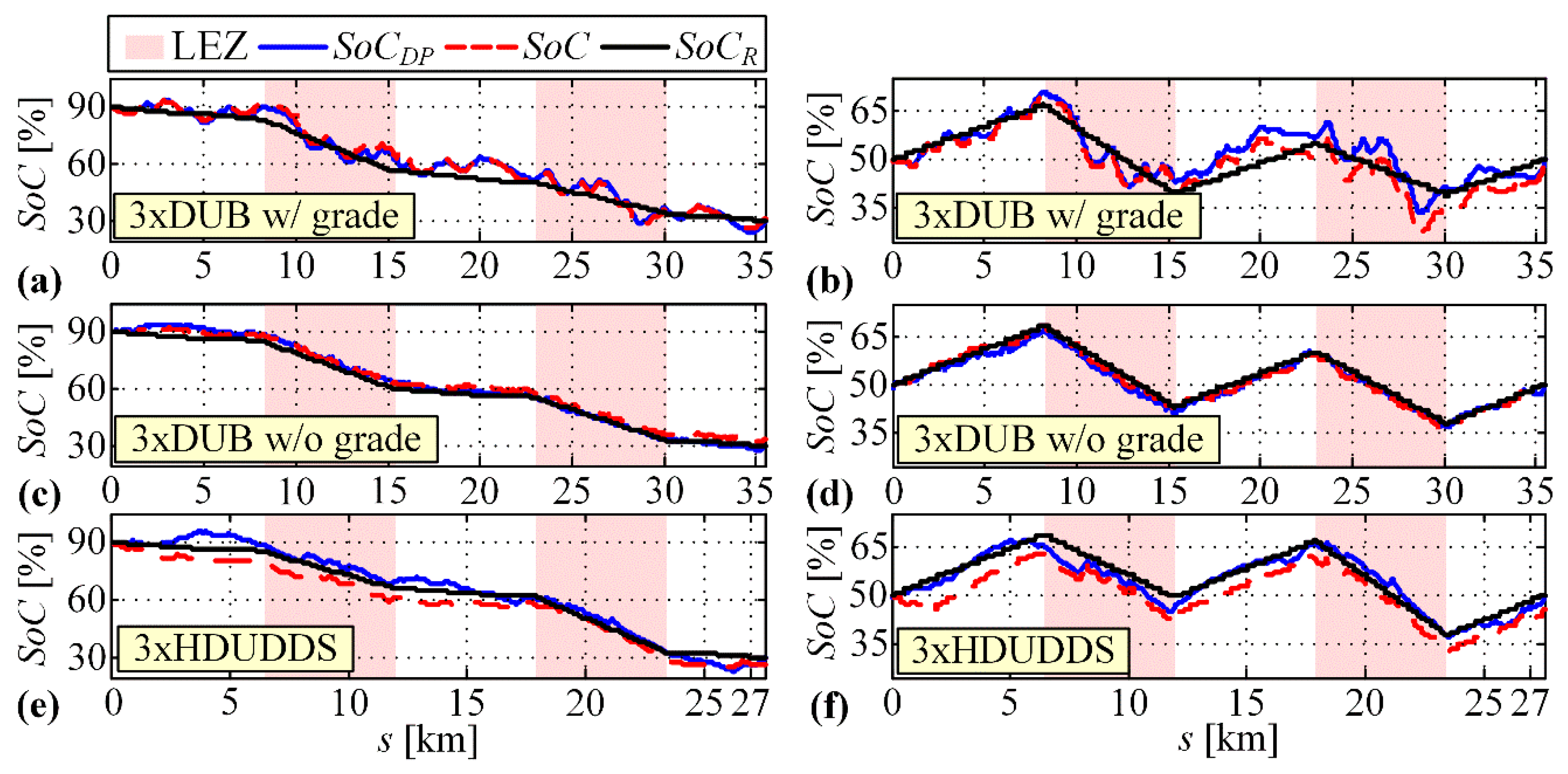
5. Simulation Results

The developed PHEV control strategy including SoC reference trajectory synthesis has been examined by backward model-based simulations for different driving cycles, zero and varying road grade profiles, and without and with LEZ presence. The obtained simulation results are compared with the globally optimal DP results.
Figure 14 shows the total fuel consumption V f for the basic case of no LEZ, and CD/CS and blended (BLND) operating regimes. The initial and target final SoC values are set to S o C i = 90 % and S o C f = 30 % , respectively, and the linear SoC reference trajectory calculated by Equation (18) is inputted into the control strategy. Since the final SoC values in simulation results do not fall exactly at the target value of 30%, the DP optimizations have been conducted for several final SoC values around 30% (black circles in Figure 14), and the results are linearly interpolated (green lines in Figure 14) [24]. This makes the simulated fuel consumptions directly comparable to the DP results. The results in Figure 14 reveal that in the blended mode the proposed control strategy approaches the DP benchmark within a margin of 2%, while in the case of CD/CS regime this margin grows to 5%. Exceptionally, in the case of 6xDUB w/grade driving cycle, the fuel consumptions are comparable for CD/CS and blended regimes. This may be explained by the influence of varying road grade considered in this case, which results in distorted and thus more similar blended and CD/CS SoC profiles, and finally in more similar total fuel consumption values.
Figure 15 shows the simulation results for the case of LEZ presence, different driving cycles (with zero or varying road grade), and different sets of initial and final SoC values. The blended regime is considered here and further on. The simulation-obtained SoC trajectories are given by red dashed lines, and they are plotted along with the DP optimal trajectories (blue lines) and the reference trajectories obtained based on Equation (21) (full black lines). The presented results point to accurate tracking of the SoC reference trajectory, thus confirming the effectiveness of the overall control strategy, including the combined, feedback and feedforward SoC controller and the SoC reference trajectory synthesis. It is important to note that in the case of varying road grade (Figure 15a,b), the actual SoC trajectories aligns much better with the DP optimal trajectories than the reference ones. This is explained by numerous battery recharging events caused by regenerative braking due to frequent negative road slopes, in which case both control strategy and DP optimizer tend to maximize regenerated energy, thus causing the SoC to deviate from its reference trajectory. This indicates that, although the synthesized piecewise linear SoC trajectory represents a relatively rough approximation of the DP optimal SoC trajectory, this reference can effectively be used in order to achieve nearly optimal results.
Table 1 gives the fuel consumption results corresponding to the simulation results from Figure 15, which are compared with respect to DP benchmark based on the interpolated DP results. The results are given and analyzed for three characteristic SoC reference trajectory synthesis cases: (i) the exact DP-obtained value of total LEZ-wise SoC depletion Δ S o C L E Z , Σ is used for each driving cycle (see Equation (21)), (ii) average value of Δ S o C L E Z , Σ for the three considered driving cycles is employed, and (iii) Δ S o C L E Z , Σ is doubled with respect to the average value of the three considered driving cycle. The motivation for this analysis is to test robustness with respect to error of estimating the driving cycle-dependent LEZ depletion Δ S o C L E Z , Σ . The results shown in Table 1 indicate that when using the exact values of Δ S o C L E Z , Σ in the SoC reference trajectory synthesis, the control strategy approaches the DP benchmark with a margin of 2%. This margin is only slightly increased in other two cases, thus confirming the robustness of the proposed SoC reference trajectory synthesis method.
Finally, the simulation verification has been conducted for different varying road grade profiles, including the recorded one (Figure 4b) and sinusoidal ones (Figure 6; no-LEZ case is considered). Two characteristic cases of SoC reference trajectory synthesis are analyzed: (i) the simple-to-implement, linear trajectory determined by Equation (18), and (ii) the trajectory synthesized according to Equations (22)–(26) which assumes prior knowledge of driving cycle features. Figure 16 shows the comparative SoC trajectories obtained by control system simulations and DP optimizations. These results indicate that the two SoC reference trajectory synthesis methods give similar SoC trajectories in the cases of recorded and high-frequency sinusoidal road grade profiles. However, these trajectories diverge from each other as the spatial frequency of road grade profile decreases. This effect is particularly emphasized in the case of lowest frequency (Figure 16b), where the SoC trajectory related to linear reference trajectory starts to deviate very early from the DP optimal trajectory. On the other hand, when the more sophisticated reference trajectory synthesis is used, the SoC trajectory follows the DP optimal one very accurately during the whole driving cycle.
Figure 17 outlines the fuel consumption values corresponding to the simulation results shown in Figure 16. The performance delivered by the control strategy approaches the DP benchmark within the margin of 2% for the recorded and high-frequency road grade profiles. Here, the fuel consumption is only slightly higher if the simplified linear SoC reference trajectory is employed when compared to the nonlinear synthesis method (see Figure 13). The difference between the results related to the use of two synthesis methods becomes higher if the mid-frequency road grade profile is considered. The largest benefit of using the nonlinear SoC reference trajectory is observed in the case of low-frequency road grade profile, where the fuel consumption is increased by 2.04% when compared to DP optimization, while in the case of linear reference trajectory, this margin equals 15.67%.

6. Conclusions

The paper has proposed a method for synthesis of optimal battery state-of-charge (SoC) trajectory for a P2 parallel plug-in hybrid electric vehicle (PHEV), which assumes a blended regime of powertrain operation. The SoC synthesis method has been verified by means of backward-looking PHEV model simulations, where different scenarios and SoC synthesis approaches are analyzed, and the obtained results are compared against DP optimized benchmark in terms of total fuel consumption.
First, the overall control strategy has been verified for the basic scenario of no low-emission zones (LEZ) and zero road grade. Here, the simple linear SoC trajectory, starting from the initial SoC and ending at its target final value, is used as a reference to the control strategy SoC controller. In this case the control strategy operating in the blended regime approaches the DP benchmark within the margin of 2%. This margin increases to 5% if the elementary, charge depleting/charge sustaining (CD/CS) regime is considered.
Next, the SoC synthesis method has been extended to deal with the LEZ presence. Here, it has been found that the optimal pattern of the SoC trajectory is linear within specific (LEZ or no-LEZ) segments, i.e., piecewise linear all over the travelling distance. The control strategy again approaches the DP benchmark to the margin of 2%. Apart from the knowledge of total driving distance, the synthesis method assumes the knowledge of total SoC depletion within LEZs, which depends on driving cycle features. Therefore, the synthesis method has been tested with respect to errors of estimating the LEZ-wise SoC depletion, which shows minor influence on fuel consumption, thus confirming the method robustness.
Finally, the SoC synthesis method has been generalized to driving cycles with varying road grade. Here, the simple linear SoC reference trajectory was firstly used. Then, the more sophisticated nonlinear SoC reference trajectory was synthesized assuming prior knowledge of power demand and vehicle velocity. The linear reference trajectory was shown to be nearly optimal only for road grade profiles characterized by mid-high spatial frequencies. However, in the case of low-frequency road grade profile (i.e., for long successive hill climbing and hill descending distances), the nonlinear SoC reference trajectory synthesis method shows the superior performance, which is close to that achieved for less hilly roads (about 2% higher fuel consumption compared to the DP benchmark is obtained, while for the linear SoC reference trajectory this margin increases to 16%).
Future work will be directed towards the synthesis of optimal SoC reference trajectory based on prediction of driving cycle features, which is anticipated to be beneficial for driving cycles with segmented driving patterns (e.g., highway/city and/or uphill/downhill driving).

Author Contributions

Conceptualization, J.D., B.Š.; Methodology, J.S., B.Š., J.D.; Software, J.S.; Validation, J.S., B.Š., J.D.; Writing-Original Draft Preparation, B.Š., J.S.; Writing-Review & Editing, J.D.; Supervision: J.D., B.Š.

Funding

It is gratefully acknowledged that this work has been supported by the Croatian Science Foundation under the project No. IP-2018-01-8323 (Project Acronym: ACHIEVE; web site: http://achieve.fsb.hr/).

Conflicts of Interest

The authors declare no conflicts of interest.

Appendix A. PHEV City Bus Parameters

A.1. Model Parameters

Vehicle parameters [15]: wheel radius, r w = 0.481 m; bus frontal area, A f = 7.52 m2; aerodynamical drag coefficient, C d = 0.70; rolling friction coefficient, R 0 = 0.01; empty bus weight, M v = 12635 kg, final drive ratio, i o = 4.72.
Battery parameters: Q m a x = 30 Ah, E m a x = 19 kWh.
Transmission gear ratios [15]:
Gear no.1.2.3.4.5.6.7.8.9.10.11.12.
Gear ratio14.9411.739.047.095.544.353.442.702.081.631.271.00

A.2. DP Optimization Parameters

Weighting coefficients: K g = 10 12 , K f = 10 6 , K L E Z = 10 3 , K S o C = 5 × 10 5 .
Constraints: S o C m i n = 0.2 , S o C m a x = 1 , P b a t t , m i n = 150 kW, P b a t t , m a x = 150 kW, ω e , m i n = 0 rad/s, ω M G , m i n = 0 rad/s, ω e , m a x = 277.5 rad/s, ω M G , m a x = 277.5 rad/s.

A.3. Control Strategy Parameters

r 0 = 0.6 , t t h = 1 s, P o f f = 75 kW, P o n = 85 kW.

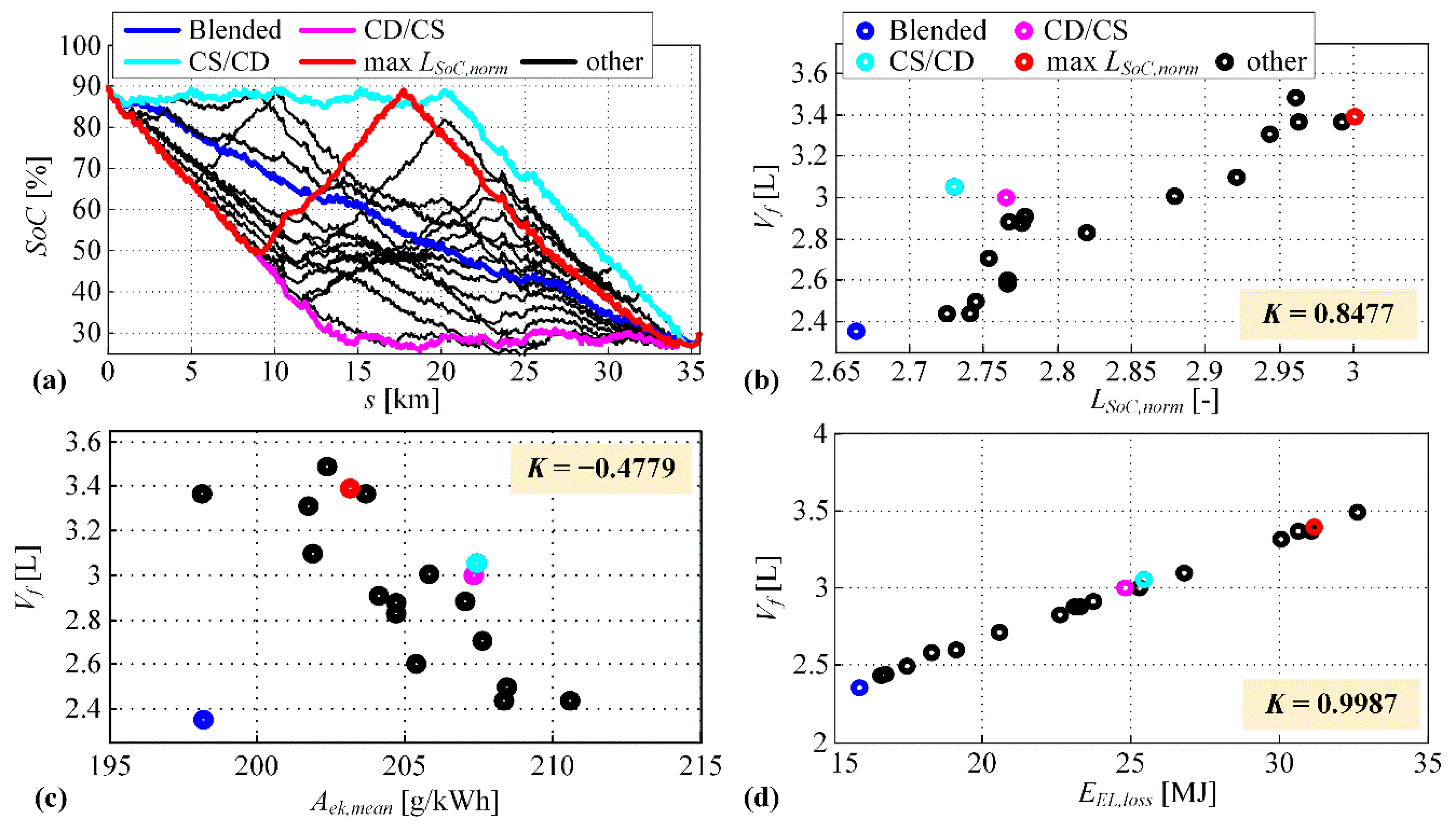
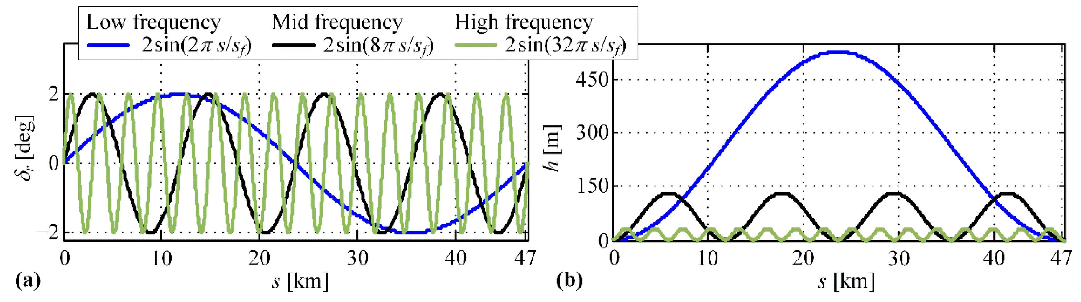
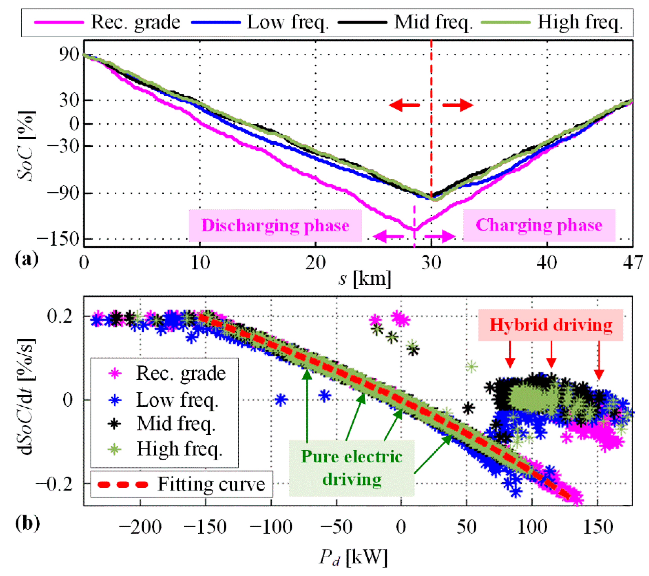
Appendix B. Analysis of Optimal SoC Trajectory Pattern

In order to further confirm the posed hypothesis on shortest-length optimality of the SoC trajectory when expressed with respect to travelled distance (Section 4), additional DP optimizations generating SoC trajectories of different length are conducted (more detailed analysis is presented in [28]). To this end, the following additional SoC-related soft constraints are added to the DP cumulative cost function (10):
J S o C , a d d = j ( S o C c o n s t r , j x j ) 2 = j K S o C ( S o C c o n s t r , j f ( x j 1 , u j 1 , v j 1 ) ) 2 , j C a
where S o C c o n s t r , j is the SoC constraint in the jth discrete time step, C a is the set of discrete time steps for which the additional SoC constraints are imposed, and K S o C is the penalization factor related to SoC constraint violation (set to 5·105, herein). The normalized SoC trajectory length is defined as
L S o C ,   n o r m = k = 1 N Δ S o C k 2 + ( Δ s k s f ) 2 ,
where the travelled distance within kth discrete time step Δ s k is normalized with respect to the total travelled distance s f .
The total electric losses, including both battery and M/G machine losses, are defined as:
E E L , l o s s = E b a t t , l o s s + E M / G , l o s s .
The battery losses have quadratic dependence with respect to battery current (i.e., E b a t t , l o s s =   I b a t t 2 R d t ) and they are dissipated as a heat on the internal battery resistance (see Figure 3a). Due to this quadratic energy loss dependence, from the battery perspective the optimal discharging from initial to final SoC is related to constant current condition, which finally results in the SoC trajectory of minimum length (this can be easily proven by using Jensen’s inequality applied to the convex function describing total battery losses; see [28] for more details). While the M/G machine losses depend on the M/G machine efficiency map (see Figure 2b), they usually dominantly relate to quadratic Ohmic losses similarly as in the battery case.
Figure A1 shows the optimization results obtained by DP optimization for different randomly generated additional SoC constraints (A1) and 3xDUB driving cycle without road grade. The obtained optimal SoC trajectories are shown in Figure A1a, among which several characteristic ones are highlighted: Blended which is generated without additional SoC constraints (the same trajectory already shown in Figure 7a), CD/CS where the battery is discharged to the lower limit of 30% as fast as possible, CS/CD where the battery discharging is maximally postponed, and max L S o C ,   n o r m whose trajectory length is maximal. All of these SoC trajectories start and finish at the same SoC values (90% and 30%, respectively), thus enabling direct comparison of obtained total fuel consumptions.
Figure A1b indicates very high correlation of the total fuel consumption with respect to the normalized SoC trajectory length given by Equation (A2), which is in line with the posed hypothesis that the SoC trajectory length should be minimized in order to minimize the fuel consumption. In order to gain more in-depth insights, the fuel consumption is analyzed also with respect to: (i) mean specific fuel consumption reflecting the engine-related losses (Figure A1c), and total electric energy losses discussed above (Figure A1d). The results in Figure A1c,d point out that the cause of increased fuel consumption is solely related to the increased total electric energy losses (the correlation factor K in Figure A1d approaches the maximum value of 1). For most of the cases (all points except the blue one in Figure A1c), the DP optimizer pushes the engine operating points to the region with slightly higher specific fuel consumption (cf. Figure 2a), in order to minimize the electric energy losses and finally the total fuel consumption (i.e., negative correlation occurs in Figure A1c). Only the slight increase of mean specific fuel consumption for a wide range of different SoC trajectories reveals high engine flexibility in adjusting its operating points to achieve the SoC trajectory of minimum length and minimal battery losses.
Figure A1. (a) DP-optimal SoC trajectories of different length, (b) corresponding fuel consumptions V f given versus: normalized SoC trajectory length L S o C , n o r m , (c) mean specific fuel consumption A e k , m e a n and (d) total electric energy losses E E L , l o s s (3xDUB driving cycle without road grade is considered; K is the correlation index).
Energies 12 04296 g0a1

References

  1. Guzzella, L.; Sciaretta, A. Vehicle Propulsion Systems, 2nd ed.; Springer: Berlin, Germany, 2007. [Google Scholar]
  2. Škugor, B.; Cipek, M.; Deur, J. Control variables optimization and feedback control strategy design for the blended operating regime of an extended range electric vehicle. SAE Int. J. Altern. Powertrains 2014, 3, 152–162. [Google Scholar] [CrossRef]
  3. Trinko, D.A.; Wendt, E.A.; Asher, Z.D.; Peyfuss, M.; Volckens, J.; Quinn, J.C.; Bradley, T.H. An Adaptive Green Zone Strategy for Hybrid Electric Vehicle Control. In Proceedings of the ITEC 2018 IEEE Transportation Electrification Conference and Expo, Long Beach, CA, USA, 13–15 June 2018; pp. 385–388. [Google Scholar]
  4. Soldo, J.; Skugor, B.; Deur, J. Optimal Energy Management Control of a Parallel Plug-In Hybrid Electric Vehicle in the Presence of Low-Emission Zones. SAE Technical Paper 2019-01-1215. 2019. Available online: https://www.sae.org/publications/technical-papers/content/2019-01-1215/ (accessed on 6 October 2019). [CrossRef]
  5. Onori, S.; Tribioli, L. Adaptive Pontryagin’s Minimum Principle supervisory controller design for the plug-in hybrid GM Chevrolet Volt. Appl. Energy 2015, 147, 224–234. [Google Scholar] [CrossRef]
  6. Martinez, C.M.; Hu, X.; Cao, D.; Velenis, E.; Gao, B.; Wellers, M. Energy Management in Plug-in Hybrid Electric Vehicles: Recent Progress and a Connected Vehicles Perspective. IEEE Trans. Veh. Technol. 2017, 66, 4534–4549. [Google Scholar] [CrossRef]
  7. Yu, H.; Kuang, M.; McGee, R. Trip-oriented energy management control strategy for plug-in hybrid electric vehicles. IEEE Trans. Control Syst. Technol. 2014, 22, 1323–1336. [Google Scholar]
  8. Ambuhl, D.; Guzzella, L. Predictive reference signal generator for hybrid electric vehicles. IEEE Trans. Veh. Technol. 2009, 58, 4730–4740. [Google Scholar] [CrossRef]
  9. Liu, Y.; Li, J.; Qin, D.; Lei, Z. Energy management of plug-in hybrid electric vehicles using road grade preview. In Proceedings of the IET International Conference on Intelligent and Connected Vehicles (ICV 2016), Chongqing, China, 22–23 September 2016. [Google Scholar]
  10. Gaikwad, T.; Asher, Z.; Liu, K.; Huang, M.; Kolmanovsky, I. Vehicle Velocity Prediction and Energy Management Strategy Part 2: Integration of Machine Learning Vehicle Velocity Prediction with Optimal Energy Management to Improve Fuel Economy. Available online: https://www.sae.org/publications/technical-papers/content/2019-01-1212/ (accessed on 6 October 2019).
  11. Xie, S.; Li, H.; Xin, Z.; Liu, T.; Wei, L. A pontryagin minimum principle-based adaptive equivalent consumption minimum strategy for a plug-in hybrid electric bus on a fixed route. Energies 2017, 10, 1379. [Google Scholar] [CrossRef]
  12. Xie, S.; Hu, X.; Xin, Z.; Brighton, J. Pontryagin’s Minimum Principle based model predictive control of energy management for a plug-in hybrid electric bus. Appl. Energy 2019, 236, 893–905. [Google Scholar] [CrossRef]
  13. Bouwman, K.R.; Pham, T.H.; Wilkins, S.; Hofman, T. Predictive Energy Management Strategy Including Traffic Flow Data for Hybrid Electric Vehicles. IFAC-PapersOnLine 2017, 50, 10046–10051. [Google Scholar] [CrossRef]
  14. Sun, C.; Moura, S.J.; Hu, X.; Hedrick, J.K.; Sun, F. Dynamic Traffic Feedback Data Enabled Energy Management in Plug-in Hybrid Electric Vehicles. IEEE Trans. Control Syst. Technol. 2015, 23, 1075–1086. [Google Scholar]
  15. Soldo, J.; Škugor, B.; Deur, J. Optimal Energy Management and Shift Scheduling Control of a Parallel Plug-in Hybrid Electric Vehicle. In Proceedings of the Powertrain Modelling and Control Conference (PMC 2018), Loughborough, UK, 10–11 September 2018. [Google Scholar]
  16. VOLVO 7900 ELECTRIC HYBRID SPECIFICATIONS. Available online: https://www.volvobuses.co.uk/en-gb/our-offering/buses/volvo-7900-electric-hybrid/specifications.html (accessed on 6 October 2019).
  17. Cipek, M.; Pavković, D.; Petrić, J.Š. A control-oriented simulation model of a power-split hybrid electric vehicle. Appl. Energy 2013, 101, 121–133. [Google Scholar] [CrossRef]
  18. Staunton, R.H.; Ayers, C.W.; Marlino, L.D.; Chiasson, J.N.; Burress, B.A. Evaluation of 2004 Toyota Prius Hybrid Electric Drive System; Oak Ridge National Laboratory (ORNL): Oak Ridge, TN, USA, 2005. [Google Scholar]
  19. Yuan, Z.; Hou, S.-H.; Li, D.; Wei, G.; Hu, X. Optimal Energy Control Strategy Design for a Hybrid Electric Vehicle. Discret. Dyn. Nat. Soc. 2013, 132064. [Google Scholar]
  20. EVO ELECTRIC LTD CATALOGUE, AF-230 Motor/Generator. Available online: http://www.fordmax.in.ua/wp-content/uploads/2014/12/AF-230-Spec-Sheet-V1.pdf (accessed on 6 October 2019).
  21. Cipek, M.; Petrić, J.; Pavković, D.; Kučinić, D. A Hydraulic Component Scalability Tool based on Willans Line Method towards the Optimal Design of Hybrid Hydraulic Vehicles. In Proceedings of the 12th Conference on Sustainable Development of Energy, Water and Environment Systems (SDEWES 2017), Dubrovnik, Croatia, 4–8 October 2017. [Google Scholar]
  22. Andre, D.; Meiler, M.; Steiner, K.; Wimmer, C.; Soczka-Guth, T.; Sauer, D.U. Characterization of high-power lithium-ion batteries by electrochemical impedance spectroscopy. I. Experimental investigation. J. Power Sources 2011, 196, 5334–5341. [Google Scholar] [CrossRef]
  23. Bin, Y.; Li, Y.; Feng, N. Nonlinear dynamic battery model with boundary and scanning hysteresis. In Proceedings of the ASME 2009 Dynamic Systems and Control Conference, Hollywood, CA, USA, 12–14 October 2009; pp. 245–252. [Google Scholar]
  24. Škugor, B.; Deur, J.; Cipek, M.; Pavković, D. Design of a power-split hybrid electric vehicle control system utilizing a rule-based controller and an equivalent consumption minimization strategy. Proc. Inst. Mech. Eng. Part D J. Automob. Eng. 2014, 228, 631–648. [Google Scholar] [CrossRef]
  25. Škugor, B.; Hrgetić, M.; Deur, J. GPS measurement-based road grade reconstruction with application to electric vehicle simulation and analysis. In Proceedings of the 11th Conference on Sustainable Development of Energy, Water and Environment Systems (SDEWES 2015), Dubrovnik, Croatia, 27 September–2 October 2015. [Google Scholar]
  26. Bellman, R.E.; Dreyfus, S.E. Applied Dynamic Programming; Princeton University Press: Princeton, NJ, USA, 1962. [Google Scholar]
  27. Cipek, M.; Škugor, B.; Čorić, M.; Kasać, J.; Deur, J. Control variable optimisation for an extended range electric vehicle. Int. J. Powertrains 2016, 5, 30. [Google Scholar] [CrossRef]
  28. Škugor, B.; Soldo, J.; Deur, J. Analysis of Optimal Battery State-of-Charge Trajectory for Blended Regime of Plug-in Hybrid Electric Vehicle. In Proceedings of the International Electric Vehicle Symposium & Exhibition (EVS32), Lyon, France, 19–22 May 2019. [Google Scholar]
  29. Paganelli, G.; Delprat, S.; Guerra, T.M.; Rimaux, J.; Santin, J.J. Equivalent consumption minimization strategy for parallel hybrid powertrains. Proc. IEEE Veh. Technol. Conf. 2002, 4, 2076–2081. [Google Scholar]
  30. Liu, K.; Asher, Z.; Gong, X.; Huang, M.; Kolmanovsky, I. Vehicle Velocity Prediction and Energy Management Strategy Part 1: Deterministic and Stochastic Vehicle Velocity Prediction Using Machine Learning. Available online: https://www.sae.org/publications/technical-papers/content/2019-01-1051/ (accessed on 6 October 2019).
Figure 1. (a) Functional scheme of considered parallel PHEV powertrain, (b) idling power loss map and (c) torque/power transfer efficiency map.
Energies 12 04296 g001
Figure 2. (a) Engine specific fuel consumption map and (b) M/G machine efficiency map, including corresponding maximum torque lines (blue lines).
Energies 12 04296 g002
Figure 3. (a) Battery equivalent circuit model and (b) dependencies of open-circuit voltage U o c reconstructed from and internal resistance R with respect to SoC for LiFePO4 battery.
Energies 12 04296 g003
Figure 4. Time profiles of (a) vehicle velocity, (b) road grade and (c) bus passengers mass for city-bus recorded driving cycle DUB and (d) speed time profile of Heavy Duty Urban Dynamometer Driving Schedule driving cycle (HDUDDS) assuming zero road grade and no passengers in the bus.
Energies 12 04296 g004
Figure 5. (a) Low-emission zones (LEZ) inserted into 3xDUB driving cycle and (b) 3xHDUDDS driving cycle, expressed with respect to travelled distances.
Energies 12 04296 g005
Figure 6. (a) Sinusoidal road grade profiles for different spatial frequencies and s f = 47.3 km and (b) corresponding altitude profiles.
Energies 12 04296 g006
Figure 7. (a) Optimal SoC trajectories obtained by DP optimization and corresponding shortest-length (linear) trajectories for 3xDUB driving cycle and (b) 2xHDUDDS driving cycle and for zero road grade and no LEZ presence.
Energies 12 04296 g007
Figure 8. (a,c) Optimal SoC trajectories and corresponding shortest-length (piecewise linear) trajectories in case of LEZ presence, for S o C i = 90%, S o C f = 30% and (b,d) S o C i   = 50%, S o C f   = 50% and for 3xDUB, 3xHDUDDS driving cycles and zero road grade.
Energies 12 04296 g008
Figure 9. (a) Optimal SoC trajectories and corresponding shortest-length (piecewise linear) trajectories for 6xDUB driving cycle and (b,c) 3xDUB driving cycle in the presence of LEZs with different initial and final SoC values for recorded road grade profile from Figure 4b.
Energies 12 04296 g009
Figure 10. (a) Optimal SoC trajectories and corresponding shortest-length (linear) trajectories for 4xDUB driving cycle and recorded road grade from Figure 4b, (b) low frequency, (c) mid frequency and (d) high frequency sinusoidal road grade profiles from Figure 6a.
Energies 12 04296 g010
Figure 11. (a) Optimal SoC trajectories from Figure 10 decomposed and rearranged to battery discharging (i.e., P b a t t > 0 , d S o C / d t < 0 ) and charging sections (i.e., P b a t t < 0 , d S o C / d t > 0 ) and (b) SoC time derivative with respect to power demand P d .
Energies 12 04296 g011
Figure 12. Block diagram of combined RB controller and ECMS optimization.
Energies 12 04296 g012
Figure 13. (a) Synthesized SoC reference trajectories plotted along with DP-optimal trajectories for recorded road grade profile and (b–d) sinusoidal profiles with different spatial frequencies.
Energies 12 04296 g013
Figure 14. Total fuel consumption for CD/CS and blended regimes, plotted against DP optimal results for different driving cycles and no LEZ case.
Energies 12 04296 g014
Figure 15. DP optimal, simulated and reference SoC trajectories for case of LEZ presence, (a,b) 3xDUB w/ grade, (c,d) 3xDUB w/o grade and (e,f) 3xHDUDDS driving cycles and different sets of initial and final SoC values ((a,c,e) S o C i = 90%, S o C f = 30%, left column and (b,d,f) S o C i = 50%, S o C f = 50%, right column).
Energies 12 04296 g015
Figure 16. DP optimal and simulated SoC trajectories (the latter obtained for linear and more advanced, nonlinear SoC reference trajectories) for (a) recorded, (b) sinusoidal low frequency, (c) sinusoidal mid frequency and (d) sinusoidal high frequency road grade profiles, no LEZ case, and 4xDUB driving cycle.
Energies 12 04296 g016
Figure 17. Fuel consumption values corresponding to simulation results from Figure 16.
Energies 12 04296 g017
Table 1. Fuel consumption values corresponding to simulation results from Figure 15 and their relative differences in comparison with DP benchmark (given in brackets).
SoCi = 90%,
Target SoCf = 30%
RB+ECMS vs. DP Fuel Consumption [L]
Exact ΔSoCLEZ,ΣAverage ΔSoCLEZ,ΣDoubled ΔSoCLEZ,Σ
3xDUB w/ grade2.83 vs. 2.80 (+0.9%)2.97 vs. 2.94 (+1.0%)3.01 vs. 2.98 (+1.1%)
3xDUB w/o grade2.59 vs. 2.56 (+1.1%)2.60 vs. 2.57 (+1.2%)2.63 vs. 2.56 (+2.6%)
3xHDUDDS3.15 vs. 3.08 (+2.2%)3.10 vs. 3.02 (+2.5%)3.11 vs. 3.02 (+3.0%)
SoCi = 50%,
Target SoCf = 50%
RB+ECMS vs. DP Fuel Consumption [L]
Exact ΔSoCZ,ΣAverage ΔSoCLEZ,ΣDoubled ΔSoCLEZ,Σ
3xDUB w/ grade5.02 vs. 4.99 (+0.6%)5.01 vs. 4.98 (+0.5%)5.16 vs. 5.08 (+1.5%)
3xDUB w/o grade5.01 vs. 4.95 (+1.2%)5.10 vs. 5.04 (+1.3%)5.16 vs. 5.02 (+2.8%)
3xHDUDDS5.72 vs. 5.66 (+1.1%)5.68 vs. 5.61 (+1.3%)5.72 vs. 5.65 (+1.2%)

