Probabilistic Load Flow Algorithm of Distribution Networks with Distributed Generators and Electric Vehicles Integration

Abstract

Probabilistic Load Flow (PLF) calculations are important tools for analysis of the steady-state operation of electrical energy networks, especially for electrical energy distribution networks with large-scale distributed generators (DGs) and electric vehicle (EV) integration. Traditional PLF has used the Cumulant Method (CM) and Latin Hypercube Sampling (LHS) method. However, traditional CM requires that each input variable be independent of one another, and the Cholesky decomposition adopted by the traditional LHS has limitations in that it is only applicable for positive definite matrices. To solve these problems, taking into account the Q-MCS theory of LHS, this paper proposes a CM PLF algorithm based on improved LHS (ILHS-CM). The cumulants of the input variables are obtained based on sampling results. The probability distribution of the output variables is obtained according to the Gram-Charlier series expansion. Moreover, DGs, such as wind turbines, photovoltaic (PV) arrays, and EVs integrated into the electrical energy distribution networks are comprehensively considered, including correlation analysis and dynamic load flow analysis for EV-coordinated charging. Four scenarios are analyzed based on the IEEE-30 node network, including with/without DGs and EVs, error analysis and performance evaluation of the proposed algorithm, correlation analysis of DGs and EVs, and dynamic load flow analysis with EV integration. The results presented in this paper demonstrate the effectiveness, accuracy, and practicability of the proposed algorithm.

1. Introduction

In recent years, renewable energy sources (RES) such as distributed photovoltaic (PV) array and wind turbines have been rapidly developing on a global scale due to the increasing depletion of fossil fuels. Meanwhile, as a green and environmentally-friendly alternative, electric vehicles (EVs) are also largely adopted in daily life. However, the stochastic and intermittent characteristics of RES and EVs can potentially lead to uncertainties in the electrical energy networks, especially in the electrical energy distribution networks. Therefore, the problem of RES accommodation and EV management is becoming more of an immediate priority. The load flow calculation is considered as the basis to solve the problem, which provides initial values for many kinds of analyses. The traditional load flow calculation can only work under certain conditions for steady state operation. With distributed generators (DGs) and EV integration, traditional methods cannot be used for analysis when there is a great number of uncertainties, however, there is a strong correlation between visible light intensity and wind speed, for example, within the same area. Thus, considering the impact of the correlated random variable inputs on the distribution network is crucial [1,2].

A study of current Probabilistic Load Flow (PLF) algorithms can be mainly divided into four categories: (1) the simplified DC model [3]; (2) the AC model based on linearization [4]; (3) the AC model based on linearization based on piecewise linearization [5]; and (4) the AC model that preserves nonlinearity [6]. AC models can usually improve the precision of PLF and the most popular studies on PLF focus on the algorithms [7]. Algorithms should usually include features as follows: (1) able to find mathematical features of output random variables; (2) deal with relativity of multi-variables; (3) take less time to reach a satisfied precision; and (4) meet generalization requirements without the limitation of mathematical models, which represent difficulties and key issues. In current literature, the PLF algorithms can be classified as simulation method, approximation method, and analytical method.

A principle of a simulation method is to extract a certain number of distribution samples, to substitute the samples into deterministic calculations, and to obtain the statistical distribution of the output, which is easy to understand and thus widely applied. Applicable simulation methods include the Simple Random Sampling Monte Carlo Simulation (SRS-MCS) [8], the Important Random Sampling Monte Carlo Simulation (SIS-MCS), the Quasi-Monte Carlo Simulation (Q-MCS) [9,10], and the Latin hypercube sampling (LHS) [11]. The simulation methods take multi-sampling of the probability distribution of the node injection power to conduct the multi-time load flow calculation. Thereafter, the statistics of the state variables and the branch load flows are obtained.

An approximation method estimates the statistical characteristics of the output random variables based on the statistical characteristics of input random variables. Approximation methods mainly comprise the point estimation and second-moment methods. The method firstly constructs the corresponding estimation points from moments of the input random variables. Afterwards, it calculates the estimated point of the output random variable based on the functions between output and input variables. Finally, it adopts statistical methods to obtain numerical features and probability distribution of the output random variables [12,13]. The approximation method is fast, while the error is large.

Analytical methods mainly include the convolution method and the Cumulant Method. The Convolution Method considers whether input variables have any linear correlation, and iteratively transform the relevant variables into a set of linear combinations of independent variables through a transformation. The probability distribution is fitted by calculating the output results. Though analytic theory of methods is generally simple and easy to understand, the calculation burden can be large. Allan et al. [14] introduced the Laplace transform and fast Fourier transform to the convolution method, thereby effectively improving the computational efficiency. The cumulant is a numerical feature of random variables, which has additivity and homogeneity. When the inputs are independent and there is a linear relationship between the inputs and the outputs, the cumulant method [15] is adopted instead of the convolution method to improve the computational efficiency. However, this method may limit the research object by specifying that it must have a fixed topology, or requiring the inputs to be independent. Work in [16] proposed a PLF algorithm based on a combination of Monte Carlo Sampling (MCS) and the cumulant method. However, the MCS requires a large number of samples to make the results accurate. Paper [17] considers that connection of electric vehicles to distribution networks, but using probabilistic Monte Carlo method alone, it is inefficient. Paper [18] further proposed an algorithm based on the Latin hypercube sampling. This method combined Cholesky decomposition to deal with the correlation of input variables, and introduced a piecewise linearized load flow model to improve accuracy. However, Cholesky decomposition is only suitable for positive definite matrices.

Taking into account correlations between the probabilistic sources, paper [19] constructed the autoregressive moving average (ARMA) model and improved the Vine-Copula theory. A joint distribution model for wind and PV power was built with measured data to capture the spatial and temporal correlations between wind and solar plants. The representative scenarios for RES were explored. A probabilistic dynamic load flow (PDLF) model based on the Joint-Moments Method (JMM) was proposed in [20]. In comparison to existing approaches, JMM permits different correlations among wind sources, thus overcoming the limits of normal jointed sources. In order to solve probabilistic load flow with correlated variables, the Nataf transformation combined with LHS and singular value decomposition method is proposed in [21]. The correlation among input variables is considered in [22], especially the joint correlation of wind power and PV generation and bus loads is considered. Based on historical sampled wind source data, work in [23] developed a model to reduce the number of uncertain parameters in the power system model by considering the spatial correlation of wind speeds between neighboring wind farms. Paper [24] proposed a probabilistic optimal power flow (POPF) approach based on Q-MCS using the correlation of wind speeds from copula functions. Point estimated method is proposed in [25] to handle the random nature of solar irradiance, wind speed and load of consumers. Paper [26] takes into account the issue of distributed generators and electric vehicles integration, but it does not consider correlations between each other. Paper [27] proposed a method can deal with continuous variables such as wind power generation and loads, and discrete variables such as fuel cell generation.

When the time-domain issue is considered, the dynamic load flow (DLF) calculation emerges. Paper [28] presented an improved probabilistic method using moments and cumulants of random variables for electrical energy system dynamic stability studies, but did not consider correlation between nodes. Work in [29] proposed a hybrid particle swarm optimization and simulated annealing (PSO-SA) method to solve the dynamic optimal power flow (DOPF) problem. A novel second order power flow solution paradigm based on artificial dynamic models is proposed in [30], but did not consider distribution networks with distributed generators and electric vehicle integration. Paper [31] proposed a Gauss-quadrature-based PLF, acknowledging uncertainties and correlations in load, renewable generation (wind and PV), and electric vehicle charging, but did not consider load flow dynamics. In paper [32] an approach to jointly plan PEV charging stations and distributed photovoltaic (PV) power plants on a coupled transportation and power network is proposed. Furthermore, a comprehensive real-time dispatch model recognizing renewable uncertainty based on DLF is proposed in [33]. The current DLF studies are mainly related to traditional loads or RES, while EV dynamic behavior is rarely considered.

Therefore, this paper focuses on the PLF algorithm of electrical energy distribution networks with DG and EV integration. The main contributions of this paper are summarized as follows:

(1)

An improved LHS based cumulant method (ILHS-CM) PLF algorithm is proposed. The random walk theory is applied to LHS, which has high sampling efficiency and can overcome the limitations of Cholesky decomposition. The improved LHS method is used to calculate the cumulant of the input variables and the probability distribution of the output variables is obtained using Gram-Charlier series expansion, which not only solves the problem of correlation of input variables, but also inherits the advantages of cumulant PLF.

(2)

In consideration of electrical energy distribution networks with distributed wind power, solar PV and EV integration, the correlation between them is analyzed. In addition to traditional wind speed correlation of wind turbines, and the power correlation of DGs and EVs, spatial correlation is introduced to obtain the correlation matrix, based on the connection impedance of DGs and EVs. Furthermore, this paper proposes the deviation index to quantitatively describe of the impact of the correlation on PLF.

(3)

Dynamic PLF is considered with EV integration, based on the obtained probability distribution function (PDF) of PLF outputs: uncoordinated and coordinated charging of the electric vehicle are analyzed. Indicators, which describe the coordinated charging that improves the operating performance of energy networks, are proposed.

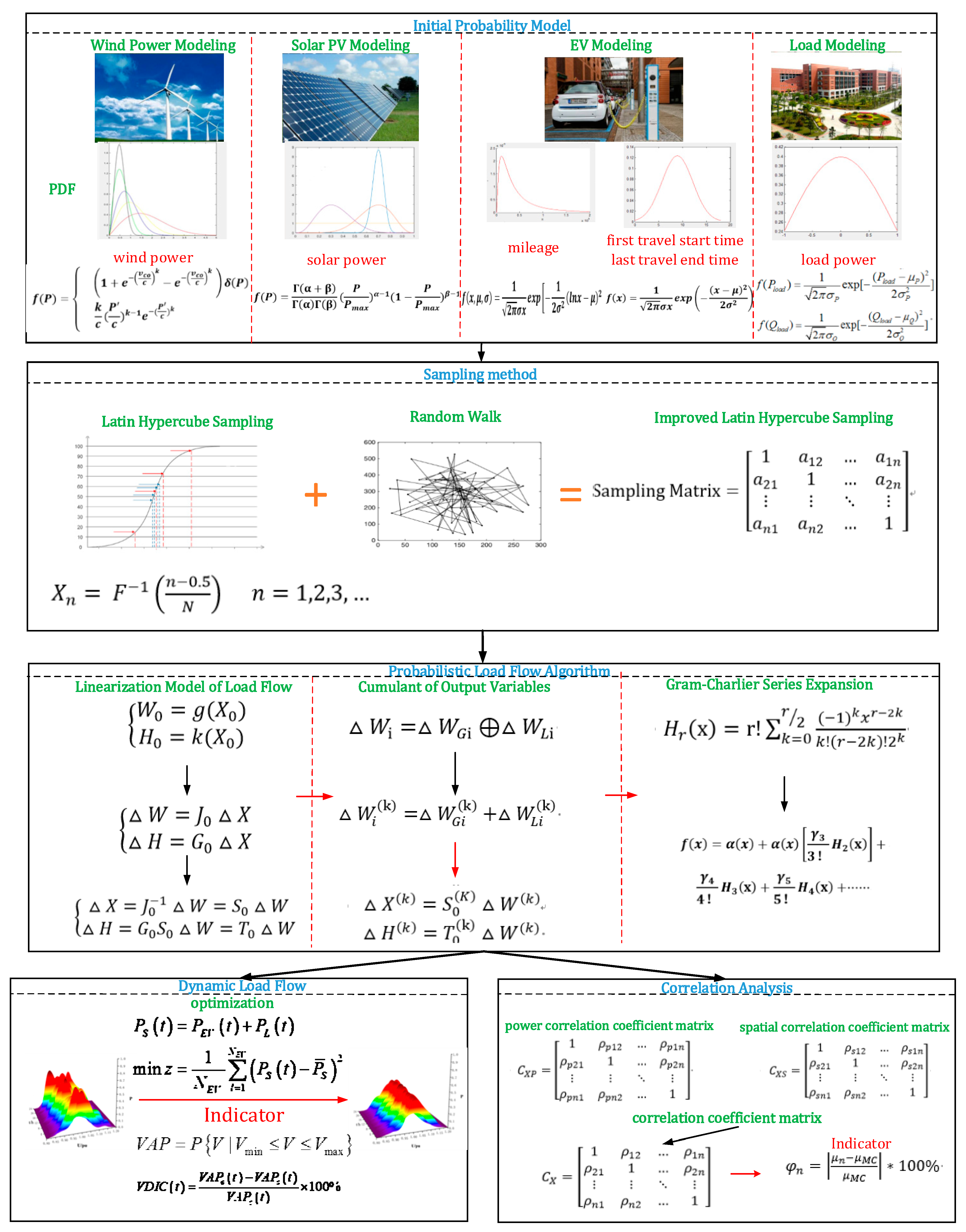
The organization of the proposed PLF algorithm is shown in Figure 1. The remainder of this paper is organized as follows: Section 2 establishes the probabilistic models of DGs and EVs. Section 3 delivers the ILHS-CM algorithm to obtain PLF calculation. In consideration of DG and EV integration in electrical energy distribution networks, Section 4 discusses correlation analysis and DLF. Four simulation scenarios are analyzed as case studies in Section 5 followed by Section 6 which concludes this paper.

2. DG and EV Probabilistic Modeling

This paper considers the probabilistic models of DGs, such as wind power and solar PV, EVs and traditional loads. The models are fitted based on historical data.

2.1. Distributed Solar PV Modeling

Light intensity obeys a Beta distribution either based on short time scales (several hours or one day) or long-time scales. The PDF model is [34]:

$$f\left(r\right)=\frac{\mathsf{\Gamma }\left(\mathsf{\alpha }+\mathsf{\beta }\right)}{\mathsf{\Gamma }\left(\mathsf{\alpha }\right)\mathsf{\Gamma }\left(\mathsf{\beta }\right)}{(\frac{r}{r_{max}})}^{\alpha -1}{(1-\frac{r}{r_{max}})}^{\beta -1}$$

(1)

where, r is the actual light intensity; $r_{max}$ is the maximum light intensity in the duration; α and β are the shape parameters of the Beta distribution; and $\mathsf{\Gamma }(·)$ is the Gamma function.

If there are n PV panels and each panel has an area of $A_i$ and the converting efficiency is ${\eta }_i$, the active power output of the panel is expressed as:

$$P=r{\displaystyle \sum }_{i=1}^n{A}_i·\frac{{{\displaystyle \sum }}_{i=1}^n{A}_i{\eta }_i}{A}$$

(2)

$$A={\displaystyle \sum }_{i=1}^n{A}_i$$

(3)

The PDF of the PV active power output can be obtained from (1) and (2):

$$f\left(P\right)=\frac{\mathsf{\Gamma }\left(\mathsf{\alpha }+\mathsf{\beta }\right)}{\mathsf{\Gamma }\left(\mathsf{\alpha }\right)\mathsf{\Gamma }\left(\mathsf{\beta }\right)}{(\frac{P}{P_{max}})}^{\alpha -1}{(1-\frac{P}{P_{max}})}^{\beta -1}$$

(4)

$$P_{max}=A\eta r_{max}$$

(5)

where, A is the total area of photovoltaic panels; $\eta$ is the photoelectric conversion efficiency; and $r_{max}$ is the maximum light intensity.

2.2. Distributed Wind Power Modeling

The Weibull distribution is adopted to model wind speed, because it is a typical distribution fitting wind speed variation with high accuracy [35]:

$$f\left(v\right)=\frac{k}{c}{\left(\frac{v}{c}\right)}^{k-1}{e}^{-{\left(\frac{v}{c}\right)}^k}v\ge 0$$

(6)

where, k is the shape parameter and c the size parameter.

The active power output characteristics of the wind turbine can be simplified as follows:

$$P=\{\begin{array}{c} 0, 0\le v\le v_{ci} \\ P_{rate}\frac{v-v_{ci}}{v_{rate}-v_{ci}}, v_{ci}\le v\le v_{rate} \\ P_{rate,} v_{rate}\le v\le v_{co} \\ 0, v_{co}\le v \end{array}$$

(7)

where, $v_{ci}$ is the cut-in wind speed; $v_{rate}$ is the rated wind speed; $v_{co}$ is the cut-out wind speed; and $P_{rate}$ is the rated output of the wind turbine.

The PDF of a wind turbine energy output can be obtained from (6) and (7):

$$f\left(P\right)=\{\begin{array}{c}0,P<0\\ \left(1+e^{-{\left(\frac{v_{co}}{c}\right)}^k}-e^{-{\left(\frac{v_{co}}{c}\right)}^k}\right)\delta \left(P\right),P=0\\ \frac{k}{c}{\left(\frac{P^{\prime }}{c}\right)}^{k-1}{e}^{-{\left(\frac{P^{\prime }}{c}\right)}^k},0<P<P_{rate}\\ 0,P>P_{rate}\end{array}$$

(8)

where, $p^{\prime }=\frac{p{v}_{rate}-p{v}_{ci}+p_{rate}{v}_{ci}}{p_{rate}}$.

2.3. Electric Vehicle Load Modeling

Based on the survey results of household car travel statistics in Northeastern China, this paper fits the data into the PDF of three kinds of cars, and uses the 24 h system to express the total load at each time of the day. The first travel start time and the last travel end time obey a normal distribution. The mileage d obeys the lognormal distribution.

The system changes the state of charge every 15 min. The number of charging periods of the charging scenario k [36] can be determined by the following formula:

$$t_k=\frac{W\ast d_k}{100\ast P_k\ast \eta }$$

(9)

where, $d_k$ is the mileage of the charging scenario k; $P_k$ is the charging power; W is the power consumption of the EV of 100 km; and$\eta$ is the charging efficiency.

Assuming that the first travel start time, the last end time, and the charging duration are independent of each other, the improved LHS technique is used to construct a scenario in which each an EV is charged every day, assuming that the sampling scale N is 1000, and finally, that the charging scenario of all EVs is obtained.

2.4. Traditional Load Modeling

This paper uses a normal distribution to reflect the time-varying of the base load:

$$f(P_{load})=\frac{1}{\sqrt{2\pi }{\sigma }_P}\exp [-\frac{{(P_{load}-{\mu }_P)}^2}{2{\sigma }_P^2}]$$

(10)

$$f(Q_{load})=\frac{1}{\sqrt{2\pi }{\sigma }_Q}\exp [-\frac{{(Q_{load}-{\mu }_Q)}^2}{2{\sigma }_Q^2}]$$

(11)

where, ${\mu }_P$ is the mean value of the load active power; ${\sigma }_p$ is the standard deviation of the load active power; ${\mu }_Q$ is the mean value of the load reactive power; and${\sigma }_Q$ is the standard deviation of the load reactive power.

3. Input Variable Cumulant Sampling

3.1. Improved Latin Hypercube Sampling Method

In this paper, the input variables for PLF are sampled by the improved LHS. Supposing that there are $L$ input variables, and the sampling frequency is $N$, the cumulative distribution function of any random variable $X_K$ is:

$$Y_K=F_K\left(X_K\right) K=1,2,3\dots \dots$$

(12)

By dividing the value interval $N$ of $Y_K$ into equal parts and taking the midpoint of each interval as the sample value of $Y_K$, the n-th sample value of $X_K$ can be obtained by the inverse function:

$$X_n= F^{-1}\left(\frac{n-0.5}{N}\right) n=1,2,3,\dots ,N$$

(13)

The $N$ sample values of each random variable are arranged in a row to generate a $K\ast N$-order LHS matrix $S_{ij}$, where i represents the i-th random variable and j represents the j-th sample of the random variable.

The traditional LHS method obtains the correlation coefficient matrix from the sampling matrix, and then performs Cholesky decomposition on the correlation coefficient matrix, and reorders the sampling matrix according to the order of decomposition.

The elements in the correlation coefficient matrix are obtained by (14):

$${\rho }_{ij}=\frac{Cov\left(L_i,L_j\right)}{\sqrt{var\left(L_i\right)var\left(L_j\right)}}$$

(14)

where, Cov(·) is the covariance; var(·) is the variance, $L_1,L_2,\dots L_i,L_j$ is each random sequence.

This paper applies the Random Walk theory to LHS. The random variables are used as the research objects, and the random walks are achieved in the sampling matrix. Since all directions are equally possible, the Random Walk method is applied to the LHS sorting step, which reduces the correlation of each random variable and ensures the randomness, parity and no preference of each sample. The sampling steps are summarized as follows:

• Set the initial iteration point $S_0$ of the LHS matrix $S_{ij}$ and the walking step $\mu$.
• In order to generate a suitable iteration number r, the initial value of a is 1.
• When a < r, random walk through the sampling matrix to generate a new matrix of j random sequences $L=\left[L_1,L_2,\dots L_i,L_j\right]$, and from the j-th new sequences, the sequence $S_1$ with the least correlation is selected by t in (15) to complete one step of random walks:

  $$\min {\rho }_r^2\left(L\right)=\frac{{{\displaystyle \sum }}_{j=2}^i{{\displaystyle \sum }}_{i=1}^{j-1}{\rho }_{ij}^2}{0.5\left(N-1\right)N}$$

  (15)
  If the calculation result is smaller than the initial value, matrix L is selected. Otherwise, a = a + 1, and return to Step 3.
• If the optimal value cannot be found for r continuous times, it means the random walk in this step does not converge. At this time, the step size $\mu$ is halved and the algorithm returns to step 1, and a new round of sorting is performed.
• A sample matrix $S_{ij}$ is generated, where i represents the i-th random variable and j represents the j-th sample of the random variable.

3.2. Cumulant Calculation for Input Variables

The traditional cumulant uses the conventional numerical method to calculate the cumulant of the input variables, which is derived from the analytical formula of the input variable PDF. The method can accurately obtain the normal distribution and the discrete distribution of the input. However, it is difficult to find other input variables with unknown distribution or distribution function. This paper proposes a method to calculate the cumulants based on an Improved LHS.

3.2.1. When the Input Variable PDF Is Known

When the PDF of the input variable W is known, N samples can be obtained according to the Improved LHS of the PDF, and then the origin moments of different orders of the input variables are calculated according to (16).

$${\alpha }_v=\frac{1}{N}{\displaystyle \sum }_{I=1}^N{X}_I^V v=1,2,3\dots$$

(16)

Then, ordered cumulants can be achieved based on the relationship between the origin moment and the cumulant of Equation (17).

$$\{\begin{array}{c}{\gamma }_1={\alpha }_1\\ {\gamma }_{v+1}={\alpha }_{v+1}-{\displaystyle \sum _{j=1}^v}{\alpha }_{v+1}-{\displaystyle \sum _{j=1}^v}{C}_v^j{\alpha }_j{\gamma }_{v-j+1} v=1,2,3···\end{array}$$

(17)

3.2.2. When the Input Variable PDF Is Unknown

When the PDF of the input variable W is unknown, the measured historical data of a certain region can be directly used as a sample, and the origin moment and the cumulant can be obtained according to Section 3.2.1. The actual electrical energy network operation can obtain a large number of discrete data measured for the input variables. The Improved LHS algorithm can directly obtain the cumulant and eliminate the correlation between random variables.

3.3. Linearization Model of Load Flow

The AC load flow model is used to represent the node injection power equation and the branch flow equation in polar form:

$$\{\begin{array}{c}W=g\left(X\right)\\ H=k\left(X\right)\end{array}$$

(18)

where, W is the node injection power; H is the branch current; X is the node voltage value.

Rewrite Equation (18) as:

$$\{\begin{array}{c}X=X_0+△X\\ W=W_0+△W\\ H=H_0+△H\end{array}$$

(19)

where, $X_0,W_0,\mathrm{and}{H}_0$ represent the expected value of the node state variable, the expected value of the node injection power, and the expected value of the branch current, respectively and meet:

$$\{\begin{array}{c}{W}_0=g\left(X_0\right)\\ H_0=k\left(X_0\right)\end{array}$$

(20)

△X is the variation of the node state variable; △W is the random disturbance of the node injection power; and △H is the variation of the branch current flow.

If (20) is performed for Taylor series expansion and ignoring the terms of second order and above:

$$\{\begin{array}{c}△W=J_0△X\\ △H=G_0△X\end{array}$$

(21)

Then, transform (21), (22) can be obtained:

$$\{\begin{array}{c}△X=J_0^{-1}△W=S_0△W\\ △H=G_0{S}_0△W=T_0△W\end{array}$$

(22)

where, $J_0$ is the Jacobian matrix; $S_0$ is the inverse matrix of $J_0$; and $G_0$ is the admittance matrix of 2b × 2n order, where b is the number of branches and n is the number of nodes, such that:

$$\{\begin{array}{c}{G}_0=\frac{\partial H}{\partial X}{|}_{X=X_0}\\ T_0=G_0{S}_0\end{array}$$

(23)

In network normal operation, the traditional Newton-Raphson load flow algorithm can be used to calculate the expected value of the node state variable $X_0$ operating at the reference point, the expected value of the branch current $H_0$ and the Jacobian matrix $J_0$, to further obtain the sensitivity matrix $S_0$ and $T_0$.

3.4. Cumulant Calculation for Output Variables

The random variable of the injection power $△W_i$ at node i can be expressed as:

$$△W_{\mathrm{i}}=△W_{G\mathrm{i}}\oplus △W_{L\mathrm{i}}$$

(24)

where, “$\oplus$” represents the convolution operation; $△W_{Gi}$ and $△W_{Li}$ represent the generator power and load power of node i.

According to the homogeneity and additivity of the cumulant method, (24) can be rewritten as the algebraic operation of the cumulant method, which can greatly simplify the calculation. The k-th order cumulant of the injection power at node i can be expressed as:

$$△W_i^{\left(\mathrm{k}\right)}=△W_{Gi}^{\left(\mathrm{k}\right)}+△W_{Li}^{\left(\mathrm{k}\right)}$$

(25)

According to the linearization model, it is derived from (22) that

$$△X^{\left(k\right)}=S_0^{\left(K\right)}△W^{\left(k\right)}$$

$$△H^{\left(k\right)}=T_0^{\left(\mathrm{k}\right)}△W^{\left(k\right)}$$

(26)

The independence of the cumulant method is determined by the nature of the convolution. Since the sampling matrix obtained with the Improved LHS has eliminated the correlation of the random variables, no further processing of the random variable is required.

3.5. Cumulant Gram-Charlier Series Expansion of Output Variables

In order to solve the PDF of voltage and power at each node, the Gram-Clarlier coefficient is calculated through the cumulants and the Gram-Clarlier series expansion is obtained. Thereafter, the PDF of output variables such as node voltage and branch current can be obtained.

The Cumulative Distribution Function (CDF) $f\left(x\right)$ can be expressed as a series expansion of the derivatives of $\alpha \left(x\right)$, and the derivative expansion of $f\left(x\right)$ is:

$$f\left(x\right)={\displaystyle \sum }_{j=0}^{\infty }{C}_j{H}_j\left(x\right)\alpha \left(x\right)=a_1\alpha \left(x\right)+a_{2}D\alpha \left(x\right)+···$$

(27)

where, x is random variable and $\alpha \left(x\right)$ is the PDF of each random variable with standard normal distribution.

$H_r\left(x\right)$ is a Schiff-Emilt polynomial, as in (28):

$$H_r\left(\mathrm{x}\right)=\mathrm{r}!{{\displaystyle \sum }}_{k=0}^{\raisebox{1ex}{$r$}\!\left/ \!\raisebox{-1ex}{$2$}\right.}\frac{{\left(-1\right)}^k{x}^{r-2k}}{k!\left(r-2k\right)!2^k}$$

(28)

The CDF of the random variables is obtained by combining (27) and (28), to obtain (29):

$$f\left(x\right)=\alpha \left(x\right)+\alpha \left(x\right)\left[\frac{{\gamma }_3}{3!}{H}_2\left(\mathrm{x}\right)\right]+\frac{{\gamma }_4}{4!}{H}_3\left(\mathrm{x}\right)+\frac{{\gamma }_5}{5!}{H}_4\left(\mathrm{x}\right)+\dots \dots$$

(29)

where, γ is the cumulant.

Finally, the PDF of the node voltage and power is obtained from the CDF. Specifically, it is expressed as the probability of each voltage and power value at a certain moment of a certain node and the maximum value of voltage and power probability at all times of a certain node on a certain day.

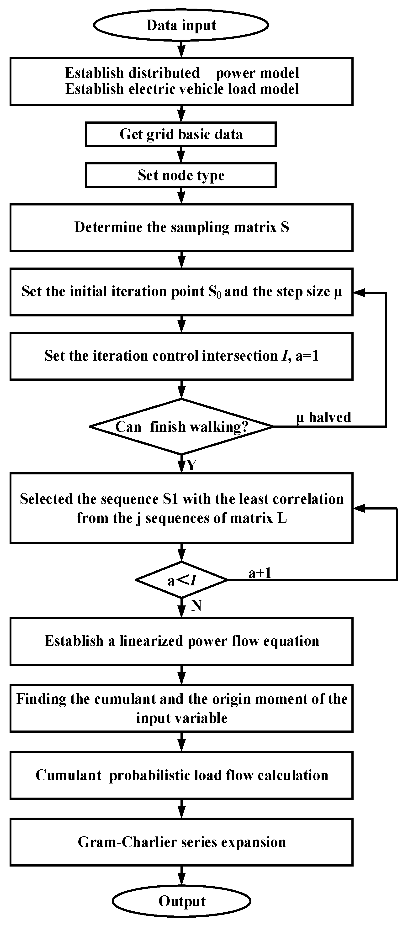
The flow chart of the ILHS-CM algorithm is shown in Figure 2. The basic steps are as follows:

• Establish the probabilistic model of DGs and random loads;
• Obtain the basic data including network node voltage, phase angle, branch active and reactive power;
• Set PQ nodes, PV nodes and the swing node;
• Obtain the sampling matrix S of input variables by improved LHS;
• Re-order the sampling matrix by the Random Walk theory;
• Perform the load flow calculation by the cumulant method;
• The output PLF results are the PDF and CDF of the output variables based on the series expansion results.

4. Correlation Analysis and Dynamic Load Flow

4.1. Correlation Indicator

The correlation of wind power, solar PV and EVs is described by the correlation coefficient matrix. Supposing the correlation coefficient matrix of n input random variables $X_1,X_2,X_3\dots X_n$ is $C_X$:

$$C_X=\left[\begin{array}{cccc}1& {\rho }_{12}& \dots & {\rho }_{1n}\\ {\rho }_{21}& 1& \dots & {\rho }_{2n}\\ ⋮& ⋮& \ddots & ⋮\\ {\rho }_{n1}& {\rho }_{n2}& \dots & 1\end{array}\right]$$

(30)

$C_X$ is obtained by the power correlation coefficient matrix $C_{XP}$ and the spatial correlation coefficient matrix $C_{XS}$.

$$C_{XP}=\left[\begin{array}{cccc}1& {\rho }_{p12}& \dots & {\rho }_{p1n}\\ {\rho }_{p21}& 1& \dots & {\rho }_{p2n}\\ ⋮& ⋮& \ddots & ⋮\\ {\rho }_{pn1}& {\rho }_{pn2}& \dots & 1\end{array}\right]$$

(31)

$$C_{XS}=\left[\begin{array}{cccc}1& {\rho }_{s12}& \dots & {\rho }_{s1n}\\ {\rho }_{s21}& 1& \dots & {\rho }_{s2n}\\ ⋮& ⋮& \ddots & ⋮\\ {\rho }_{sn1}& {\rho }_{sn2}& \dots & 1\end{array}\right]$$

(32)

where, ${\rho }_{pij}$ in (31) can be obtained by (14) and ${\rho }_{sij}$ is defined as:

$${\rho }_{sij}=y_{ij}/\max \left(y_{ij}\right)$$

(33)

where, $y_{ij}$ is the admittance between DG or EV connection node i and j.

Each element in (30) can be obtained by ${\rho }_{ij}={\rho }_{pij}\times {\rho }_{sij}$.

In order to clarify the influence of correlations on nodes, a deviation index is proposed to verify the influence of correlation on node voltage accuracy.

$${\phi }_n=\left|\frac{{\mu }_n-{\mu }_{MC}}{{\mu }_{MC}}\right|\ast 100\%$$

(34)

where, ${\phi }_n$ is the offset estimate; ${\mu }_n$ is the node voltage mean by the PLF; and ${\mu }_{MC}$ is the node voltage mean by the MCS algorithm.

4.2. Electric Vehicle Coordinated Charging

By considering that the load leveling is an optimization objective of the coordinated charging of EVs, then the objective function is:

$$\begin{array}{c}{P}_S\left(t\right)=P_{EV}\left(t\right)+P_L\left(t\right)\\ \min z=\frac{1}{N_{EV}}{\displaystyle \sum _{l=1}^{N_{EV}}{\left(P_S\left(t\right)-{\overline{P}}_S\right)}^2}\end{array}$$

(35)

where, $P_S\left(t\right)$ is the total load with EV charging power at t time; $P_L\left(t\right)$ is the total load without EV charging at t time; ${\overline{P}}_S$ is the average load and ${\overline{P}}_S={\displaystyle \sum _{t=1}^{N_{EV}}\left(P_{EV}\left(t\right)+P_L\left(t\right)\right)}/N_{EV}$. z is the objective; and $N_{EV}$ is the number of intervals for coordinated EV charging. The constraints of the optimization function can be found in [32].

EVs are normally connected in the distribution network: thus, as the load power at the connecting node increases, the voltage gradually decreases. Therefore, this paper proposes indices based on voltage PDF to describe the performance of uncoordinated charging and coordinated charging of EVs.

4.2.1. Voltage Allowable Probability

Similar to the confidence interval, the probability density between the upper and lower limits of the allowable voltage of the voltage samples is defined as the voltage allowable probability(VAP), which is shown in (36):

$$VAP=P\left\{V|V_{\min }\le V\le V_{\max }\right\}$$

(36)

where, $V$ is the voltage sample, and $V_{\min }$ and $V_{\max }$ are the upper and lower limits allowed by the voltage. $V_{\min }$ and $V_{\max }$ are generally set as −7% and 7% in the distribution network.

4.2.2. Voltage Distribution Improvement Factor

By comparing the voltage allowable probability in the case between coordinated and uncoordinated charging, and considering the dynamic probability distribution of electric vehicle charging, the voltage distribution improvement coefficient (VDIC)at t time is defined as follows:

$$VDIC\left(t\right)=\frac{VA{P}_o\left(t\right)-VA{P}_s\left(t\right)}{VA{P}_s\left(t\right)}\times 100\%$$

(37)

where, $VA{P}_s\left(t\right)$ is the voltage allowable probability with uncoordinated EV charging at t time, and $VA{P}_o\left(t\right)$ is the voltage allowable probability with coordinated EV charging at t time.

The voltage distribution improvement factor differs with the probability distribution of DLF in improving performance at different time periods. This paper takes the maximum, minimum and mean values as relevant indicators to describe the improving performance of EV coordinated charging in the electrical energy networks.

5. Case Studies

5.1. Simulation Scenario Settings

The distributed solar PV in this paper uses historical data of a region in Northeastern China. Using data fitting, the distributed solar PV meets the β distribution, the shape parameter α = 0.2274, β = 1.2995, and the installed capacity of the PV power station is 6 MW. The PV panel area is 16,000 m². The average light intensity is 1.1333 kW/m², and the photoelectric conversion efficiency $\eta$ is 13%.

According to historical data of the same region, the wind speed of the distributed wind power satisfies the Weber distribution with the scale parameter of 7.8 and the shape parameter of 3. The wind farm cut-in wind speed is 3 m/s, and the cut-out wind speed is 15 m/s. The rated wind speed is 13.5 m/s, and the rated power of each wind farm is 6 MW. The power correlation coefficient matrix, the spatial correlation coefficient matrix, and the correlation coefficient matrix of the two wind farms connected are: $C_{WP}$, $C_{WS}$, and $C_W$, respectively:

$$C_{WP}=\left[\begin{array}{cc}1& 0.8\\ 0.8& 1\end{array}\right],C_{WS}=\left[\begin{array}{cc}1& 1\\ 1& 1\end{array}\right],C_W=\left[\begin{array}{cc}1& 0.8\\ 0.8& 1\end{array}\right]$$

The random load of electric vehicles in this paper adopts the conventional slow charging mode. The first travel start time t obeys the normal distribution N (8.92, 3.242); The last travel end time t obeys the normal distribution N (17.47, 3.412); The mileage d obeys the lognormal distribution lnd~N (3.46, 1.142). The battery parameters are: 70 kW.h capacity, 15.84 kW.h per 100 km power consumption, conventional charging power of 7 kW and battery charging efficiency of 87%. It is assumed that the power battery is fully charged before daily travel.

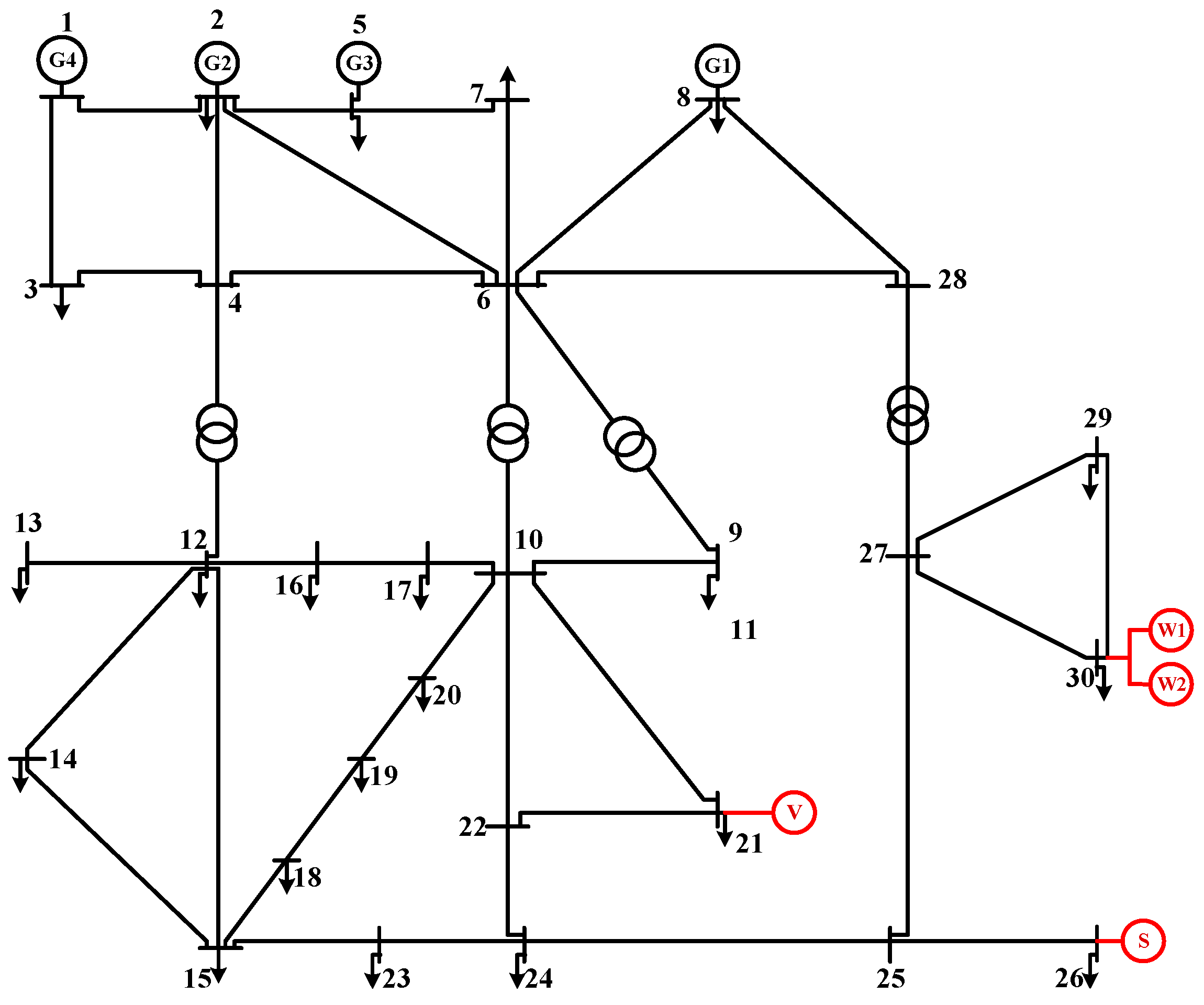
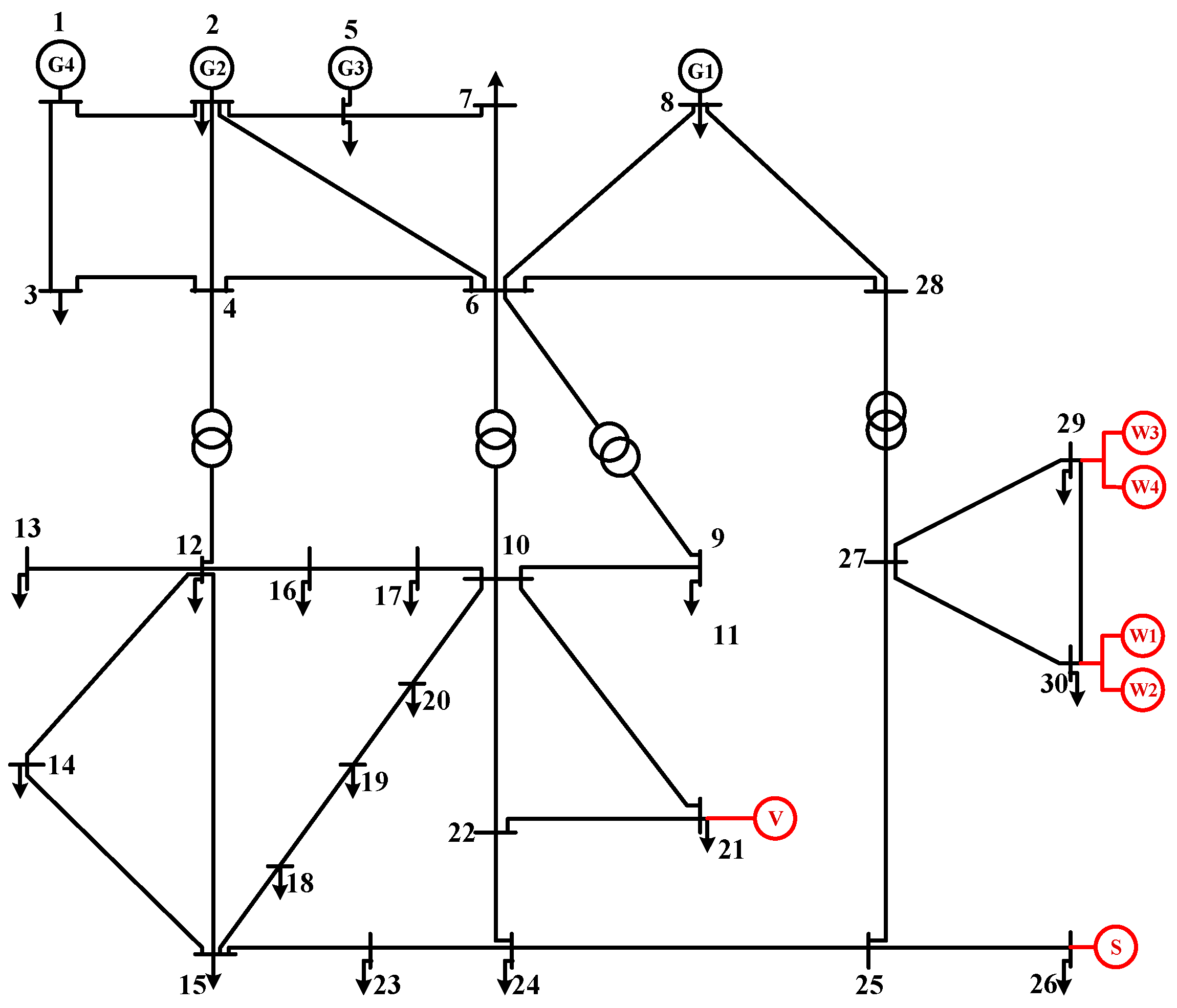
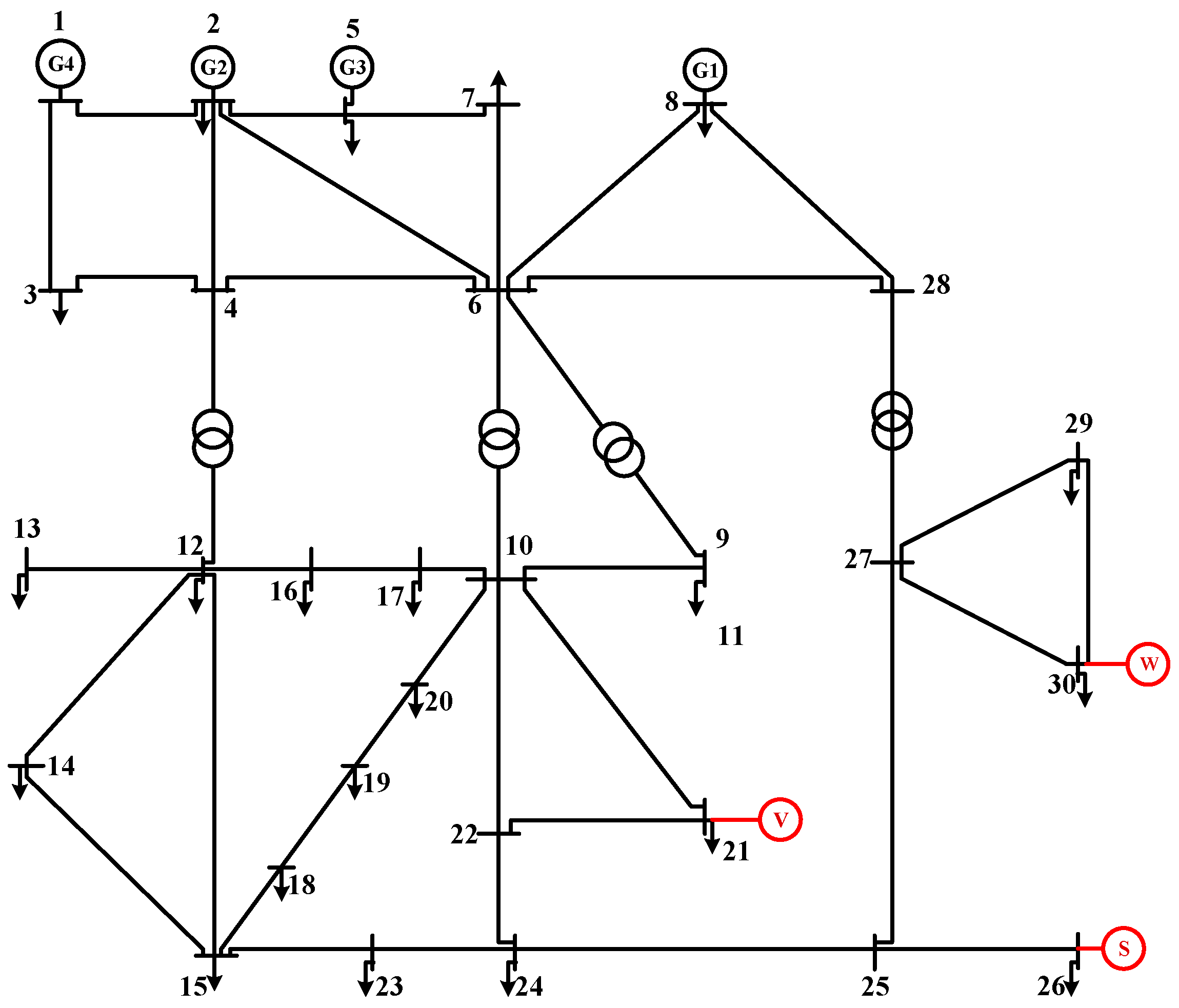
Using the IEEE-30 bus energy distribution network as an example, the topology is shown in Figure 3. The voltage reference value is 12.66 kV. Node 1 acts as the swing node, and the voltage amplitude is 1.05 pu. Node 21 is connected with EVs; Node 26 is connected with distributed solar PV; and Node 30 is connected with distributed wind power. The first 6-order cumulant of the node’s active power output obtained by the improved LHS is shown in

Table 1. Cumulant of DGs and EVs.

Active Power	Cumulant
	First Order	Second Order	Third Order	Fourth Order	Fifth Order	Sixth Order
Node 21	1.33 × 10−2	1.15 × 10−3	6.87 × 10−6	4.44 × 10−7	2.81 × 10−8	1.14 × 10−9
Node 26	2.36 × 10−2	2.15 × 10−3	1.10 × 10−5	2.31 × 10−6	6.9 × 10−8	3.17 × 10−9
Node 30	2.70 × 10−2	1.44 × 10−3	1.31 × 10−5	1.57 × 10−7	2.14 × 10−9	2.96 × 10−10

.

The simulation platform used in this paper was: An Intel Core i7-7700 2.80GHz CPU, with 16 GB memory. There are four simulation scenarios in the case study.

• Scenario 1: PLF Analysis with DGs and EVs integration;
• Scenario 2: Error Analysis and Performance Evaluation of the Algorithm;
• Scenario 3: Correlation analysis of DGs and EVs;
• Scenario 4: DLF analysis with EV integration.

5.2. Scenario 1: PLF Analysis with DGs and EVs Integration

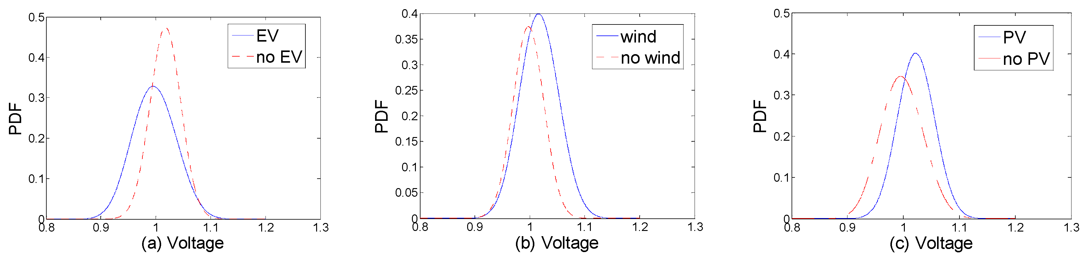
In order to analyze the impact of DG and EV integration on the electrical energy grid, the probability distribution of node voltage amplitude with and without DGs and EVs are analyzed as shown in Figure 4a–c.

It can be seen from Figure 4a that in the case of EV integration, the load power increases and the voltage amplitude is significantly reduced.

In Figure 4b,c, in the case of DG integration, the uncertainty of wind power and solar PV has increased the fluctuation of the node voltage. With DG integration, the load power decreases and there is a significant increase in the voltage amplitude.

5.3. Scenario 2: Error Analysis and Performance Evaluation of the Algorithm

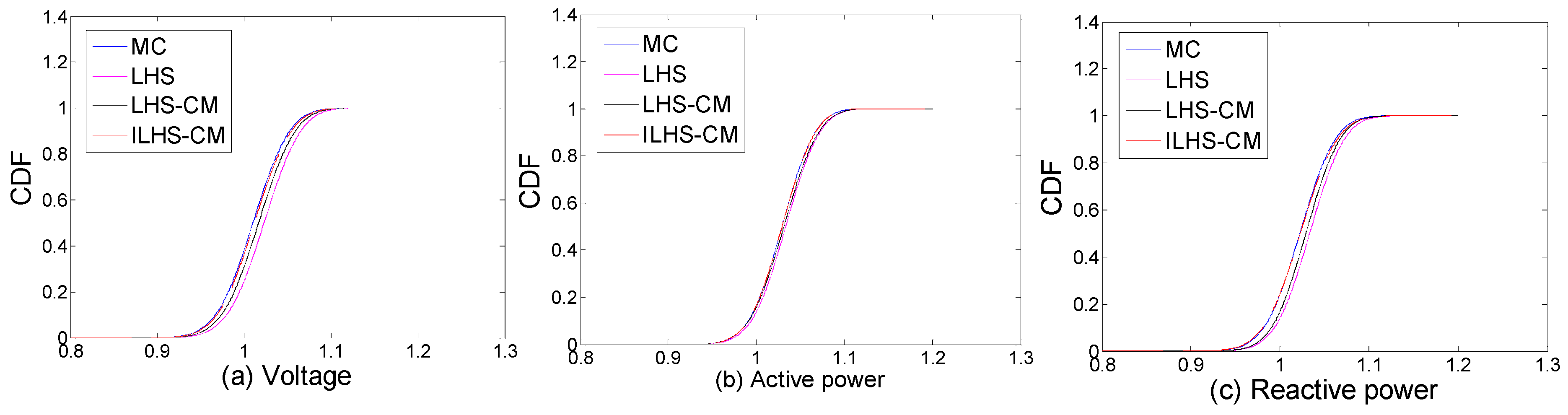
The MCS results are used as the basis to test the accuracy of the PLF results. According to the DG and EV probability model established in Section 1, the sample is obtained by 10,000 iterations of the MCS method, and then the CDF of the output variables is obtained according to the deterministic power flow calculation. The CDF is shown in Figure 5a–c.

Two indicators are used to evaluate the accuracy of the algorithm presented in this paper from different perspectives. The relative error indicator [37] of the expected value and standard deviation of the output variables of this paper are selected:

$${\epsilon }_s^y=\left|\frac{X_{sc}^y-X_{sm}^y}{X_{sm}^y}\right|\times 100\%$$

(38)

The (ARMS) of the output variables of this paper is used to describe the accuracy of the PDF characteristics of the output variables:

$${ϵ}^y=\frac{\sqrt{{{\displaystyle \sum }}_{i=1}^N{\left(C_{C_i}^y-C_{M_i}^y\right)}^2}}{N}$$

(39)

where, ${\epsilon }_s^y$ is the relative error index; and ${ϵ}^y$ is the average root mean index; y is the output variable, including the node voltage and the branch current. S is the statistical feature type, including the expected value and standard deviation; $X_{sc}^y$ and $X_{SM}^y$ are the output variable results obtained by the proposed method and the Monte Carlo method, respectively; $C_{C_i}^y$ and $C_{M_i}^y$ respectively are the i-th point on the PDF of the output variables obtained by the proposed method and the Monte Carlo method. N is the number of samples.

Table 2. Relative error indicators of output variables at Node 30.

Output Variables	${\mathit{\epsilon }}_{\mathit{s}\mathit{m}\mathit{i}\mathit{n}}^{\mathit{y}}/\mathit{\%}$		${\mathit{\epsilon }}_{\mathit{s}\mathit{m}\mathit{a}\mathit{x}}^{\mathit{y}}/\mathit{\%}$
	Expected Value	Standard Deviation	Expected Value	Standard Deviation
Voltage amplitude	0.002	0.208	0.012	0.255
Branch active power	0.125	0.211	0.189	0.329
Branch reactive power	0.432	0.453	2.882	2.635

and

Table 3. ARMS indicator of Node 30 output variable.

Output Variables	${\mathit{ϵ}}_{\mathit{m}\mathit{i}\mathit{n}}^{\mathit{y}}$	${\mathit{ϵ}}_{\mathit{m}\mathit{a}\mathit{x}}^{\mathit{y}}$
Voltage amplitude	0.235	0.540
Branch active power	0.346	1.265
Branch reactive power	0.656	4.352

deliver the results of the proposed two indicators.

It is apparent from Table 2 and Table 3 that the proposed algorithm has high accuracy. The relative error of the node voltage amplitude is rather small. The relative error of the active and reactive power is higher. However, the maximum relative error is only 2.882% for the expected value. Similar to the relative error, the voltage amplitude had the smallest ARMS, and the branch reactive power was larger, 0.656%.

Table 4. Comparison of the means of four algorithms.

Algorithms	Voltage Mean	Active Power Mean	Reactive Power Mean
MCS	0.4751	0.4273	0.4445
LHS	0.4430	0.4168	0.4257
LHS-CM	0.4586	0.4219	0.4399
ILHS-CM	0.4708	0.4255	0.4428

presents the comparison of the means of four algorithms, as in: MCS, LHS, LHS-CM, and ILHS-CM.

It can be seen from Table 4 that among the four algorithms, the mean of improved LHS-CM is the closest to MCS. In comparison with MCS, the voltage, active power, and reactive power errors of ILHS-CM are 0.91%, 0.42%, 0.38%, respectively, which proves that the inclusion of CM and random walk theory has improved the accuracy in the proposed algorithm.

In addition to the accuracy index to evaluate the validity and feasibility of the proposed algorithm, calculation time is also considered.

Table 5. Comparison of calculation time between different algorithms.

Method	Number of Samples	Calculating Time/s
MCS	10,000	624.2
ILHS-CM	500	3.5

compares the calculation time of the proposed algorithm and the 10,000-iteration traditional MCS algorithm. Under the same calculation accuracy, the results show that the calculation time of the MCS algorithm is 624.2 s, and the calculation time of the proposed algorithm is 3.5 s, which is only 1/170 of the traditional MCS algorithm. The cumulant PLF calculation using the improved LHS can accurately obtain the probability distribution of the output variables, and can inherit the advantages of the cumulant method, so that it can be further applied to the steady state analysis of the electrical energy networks.

5.4. Scenario 3: Correlation Analysis of DGs and EVs

5.4.1. Wind Speed Correlation

In order to analyze the impact of wind speed correlation on the power grid, the influence of wind speed correlation is analyzed. Four wind farms are connected at Node 29 and 30, respectively. The connection node is shown in Figure 6. It is assumed that the wind speed correlation coefficient between the four wind farms is $\rho$, and the other parameters are the same as in Section 5.1. In this case, the spatial correlation coefficient is not included.

The wind speed correlation coefficients are 0.1–0.3 (low correlation), 0.4–0.6 (moderate correlation), and 0.7–0.9 (high correlation). The changes of the mean and standard deviation of the power output and voltage amplitude of the two wind farms are used, and then the impact of wind speed correlation on the network is analyzed.

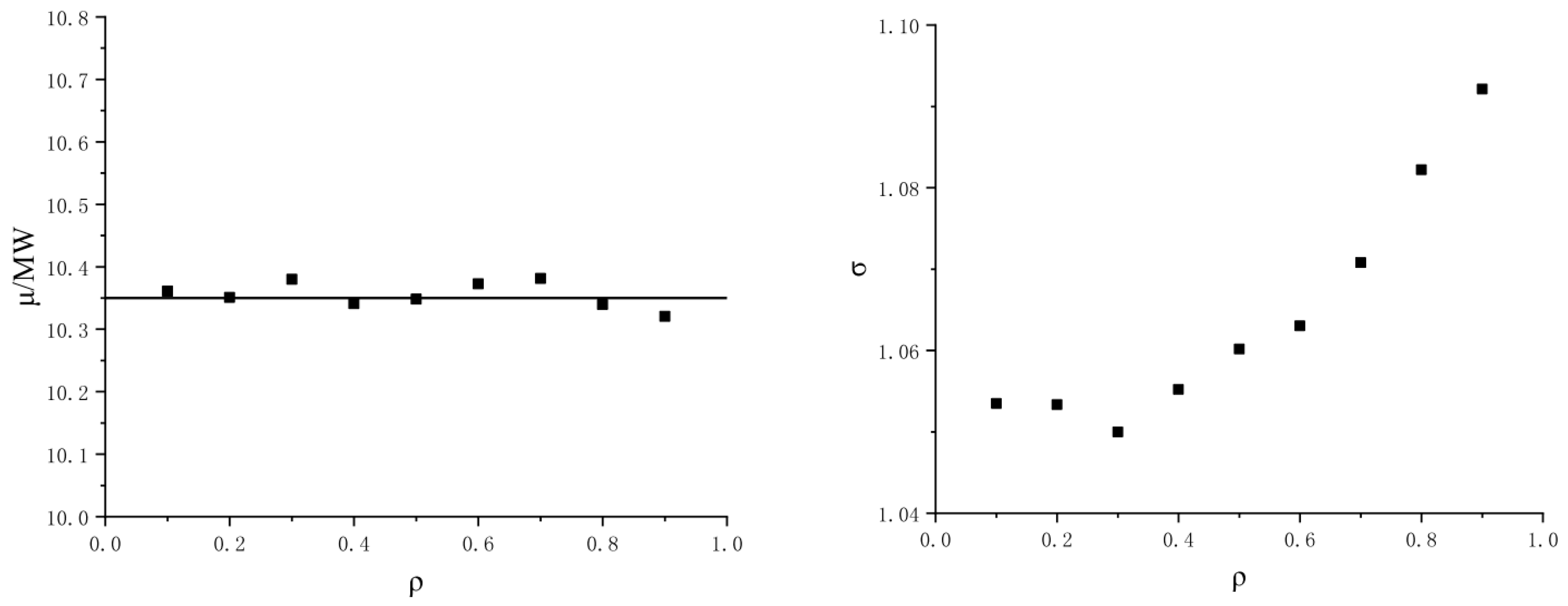
The effect of wind speed correlation on the wind power output at Node 30 is shown in Figure 7. The expected value of wind power output is little affected by the wind farm correlation, and it fluctuates around 10.35 MW. The mean square error of wind power output increases with the correlation of wind speed. In the case of low correlation, the mean square error fluctuates around 1.054, whereas with moderate correlation, the mean square error increases from 1.055 to 1.063, and the mean square error increases by roughly 0.76%. In the high correlation, the mean square error increases from 1.070 to 1.092, and the mean square error increased by roughly 2.3%.

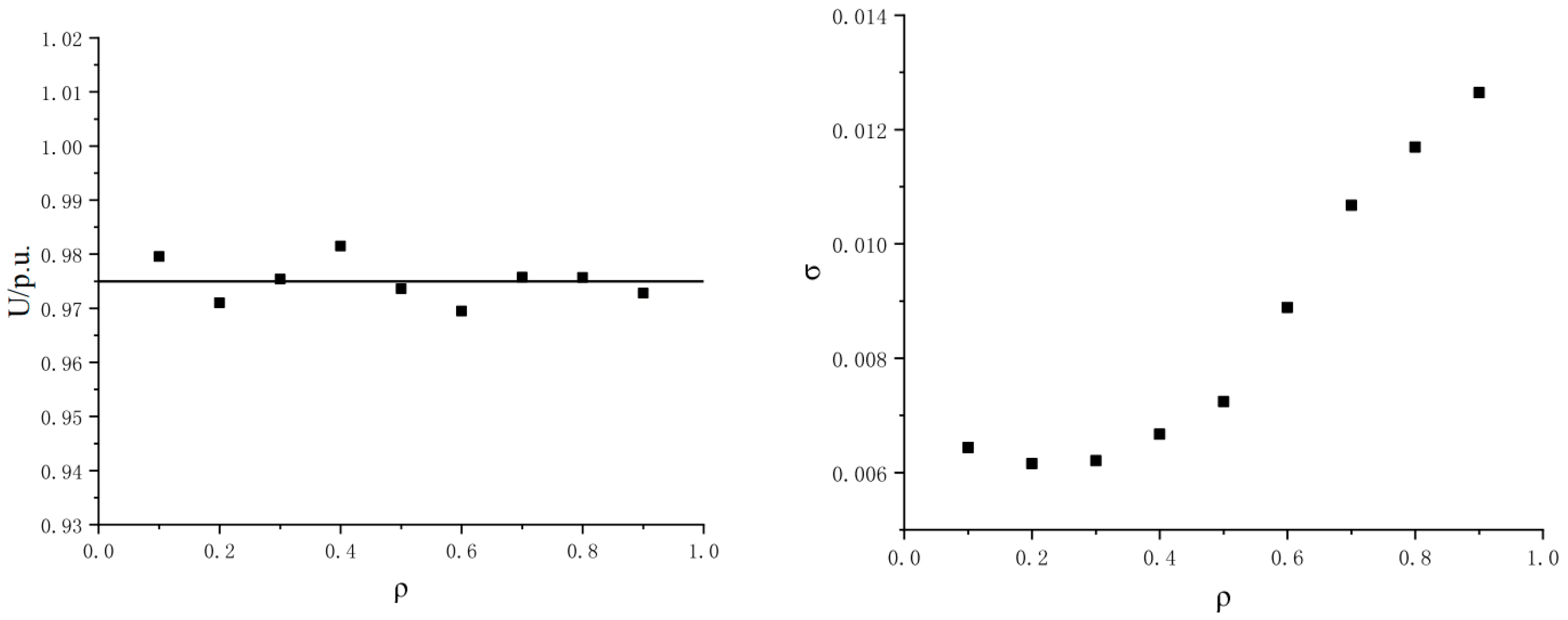
The effect of wind speed correlation on the node voltage amplitude at Node 30 is shown in Figure 8. The expected value of the voltage amplitude of Node 30 is little affected by the wind farm correlation, and fluctuates substantially around 0.975 pu. The mean square error of the voltage amplitude at Node 30 increases with the increase of wind speed correlation. In the case of low correlation, the mean square error fluctuates around 0.0065; with moderate correlation, the mean square error rises from 0.0067 to 0.013, and the mean square error increased by about 94%.

Therefore, it can be seen that the rise of wind speed correlation increases the probability of the extreme value of wind power output and the node voltage, which results in significant fluctuation of the standard deviation.

5.4.2. Correlation between DGs and EVs

In consideration of the impact of correlation between wind, solar PV, and EV integration in an electrical energy distribution network, each connection is shown in Figure 9. The power correlation coefficient matrix, the spatial correlation coefficient matrix, and the correlation coefficient matrix between the connection nodes are obtained from Equations (30)–(32).

$$C_{WP}=\left[\begin{array}{ccc}1& 0.7& 0.5\\ 0.7& 1& 0.3\\ 0.5& 0.3& 1\end{array}\right],C_{WS}=\left[\begin{array}{ccc}1& 1& 0.9\\ 1& 1& 0.8\\ 0.9& 0.8& 1\end{array}\right],C_W=\left[\begin{array}{ccc}1& 0.7& 0.45\\ 0.7& 1& 0.24\\ 0.45& 0.24& 1\end{array}\right]$$

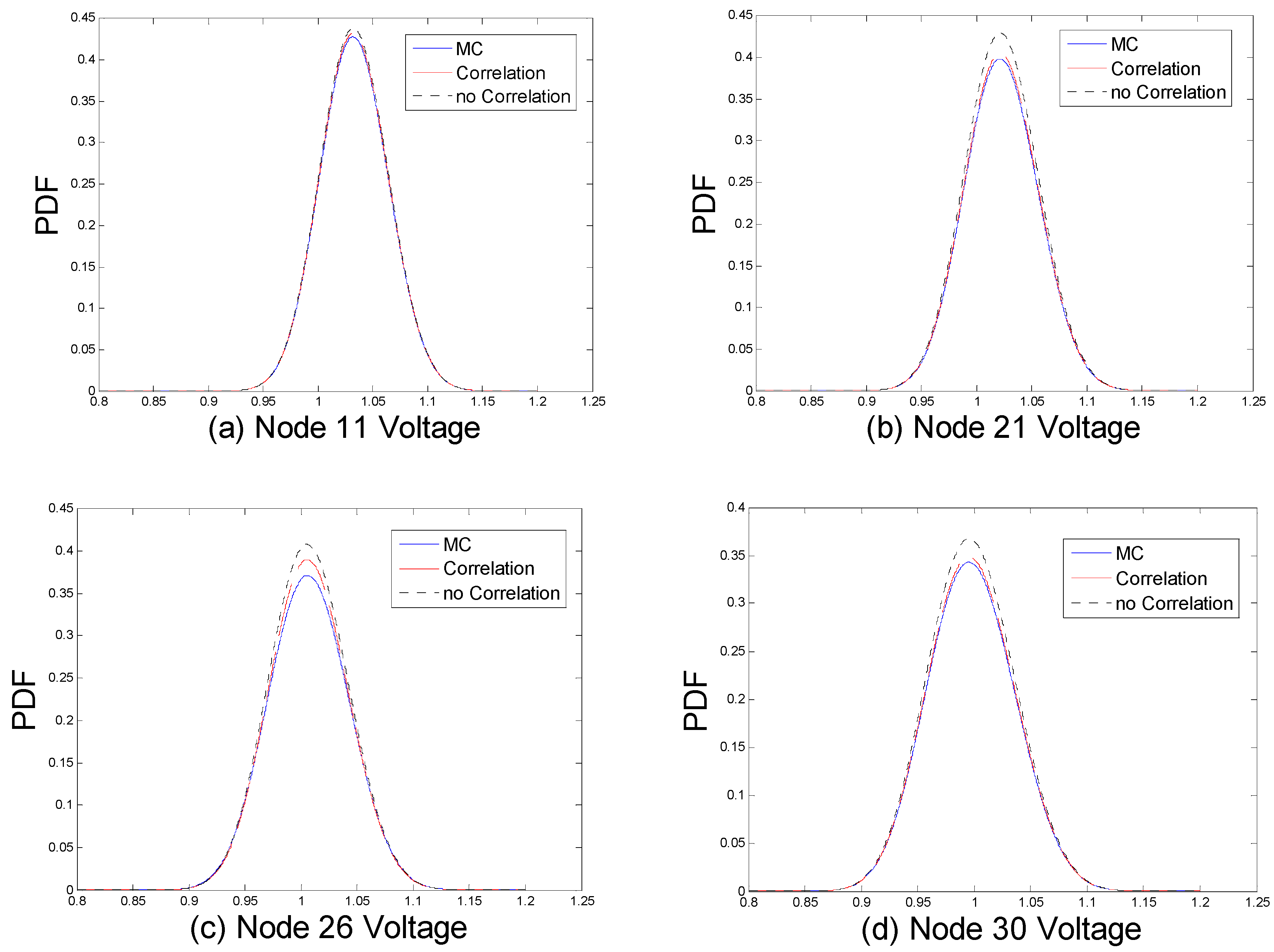
Figure 10 illustrates the PDFs of PLF results at four nodes, Node 11, 21, 26, and 30. Three algorithms are compared, including 10,000 iteration of MCS using PLF, ILHS-CM PLF with correlation, and ILHS-CM PLF without correlation.

Table 6. Deviation estimation indicators with/without correlation.

Node Number	without Correlation ${\mathit{\phi }}_{\mathit{n}}/\%$	with Power Correlation ${\mathit{\phi }}_{\mathit{n}}/\%$	with Power and Spatial Correlation ${\mathit{\phi }}_{\mathit{n}}$/%
Node 11	2.401	1.080	0.503
Node 21	6.723	2.389	1.024
Node 26	9.449	3.481	1.279
Node 30	5.522	1.691	0.660

shows the deviation estimation indicators of the voltage PDF at each node according to Equation (34).

From Figure 10 and Table 6, correlation between DGs and EVs is apparent, with the PLF results closer to 10,000 MCS iterations, which is more accurate than without the correlation. The other nodes without DG or EV integration are influenced little, when correlation is considered. The deviation estimation indicator is only about 1.4%. Moreover, the inclusion of the spatial correlation coefficient matrix renders the result more accurate.

5.5. Scenario 4: DLF Analysis with EV Integration

In order to quantitatively analyze the impact of uncertainty in EV traveling on the electrical energy network, the DLF is further studied on the basis of the traditional PLF, and the results are substituted into the objective function to obtain the coordinated charging strategy.

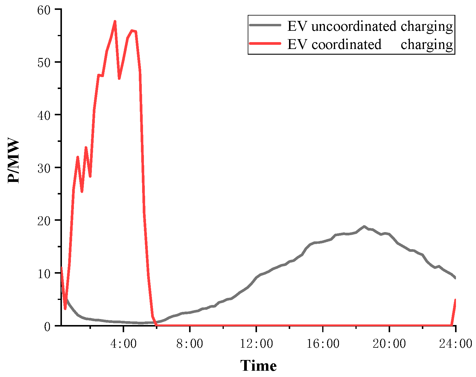
In this paper, the dynamic probabilistic characteristics of the node voltage amplitude are analyzed, with consideration of uncoordinated and coordinated charging [38]. In the case of uncoordinated charging, the owner is accustomed to charge the EV immediately after the last trip. Coordinated charging means the use of practical and effective economic or technical measures to guide and control EV charging while meeting the charging requirements of EVs. This paper focuses on load leveling [39,40]. 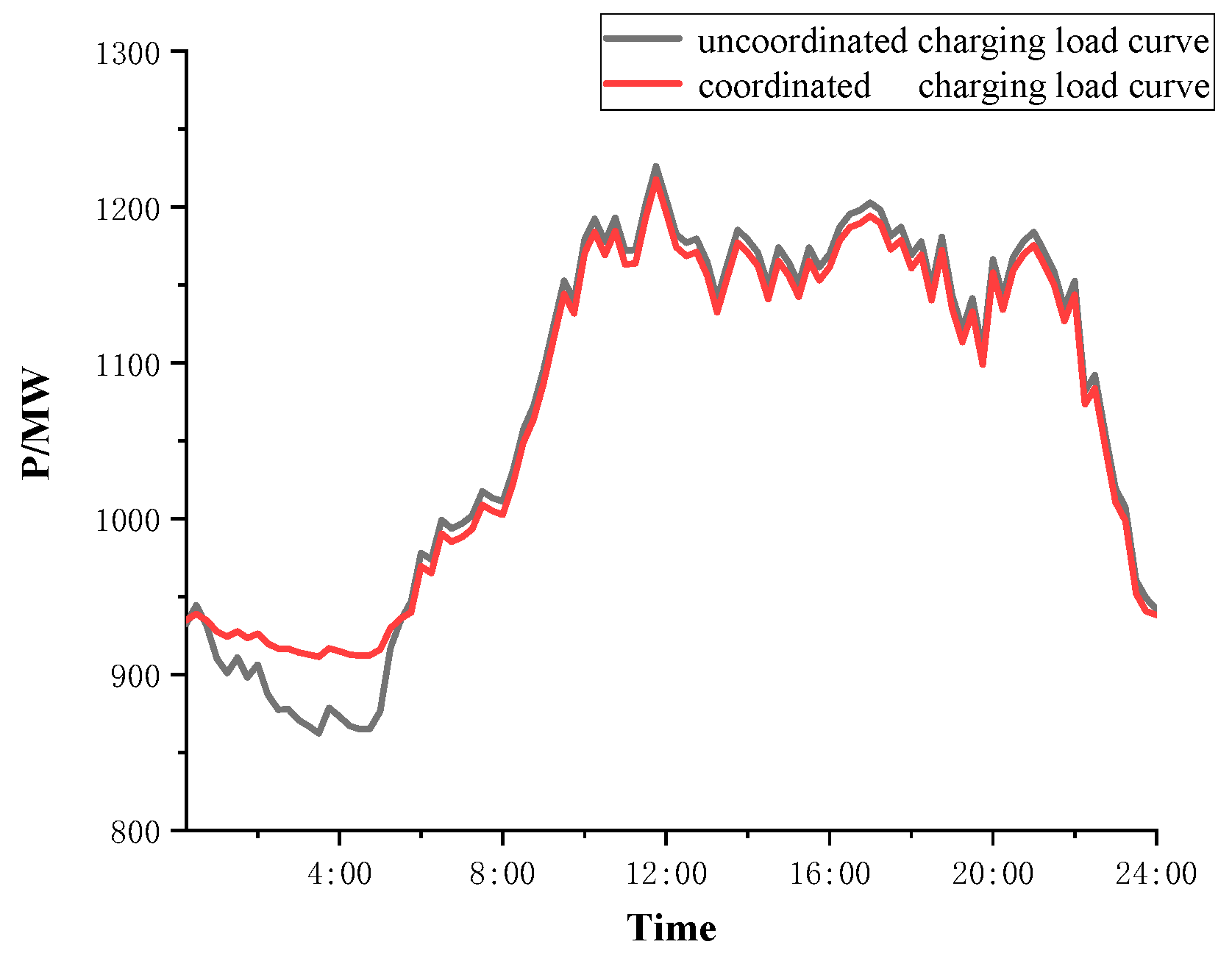The EV coordinated charging and uncoordinated charging curves are shown in Figure 11. The total load curves with EV coordinated and uncoordinated charging are shown in Figure 12.

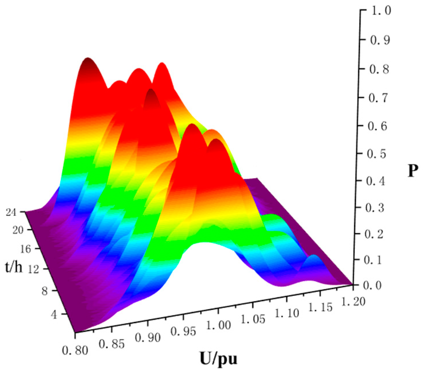
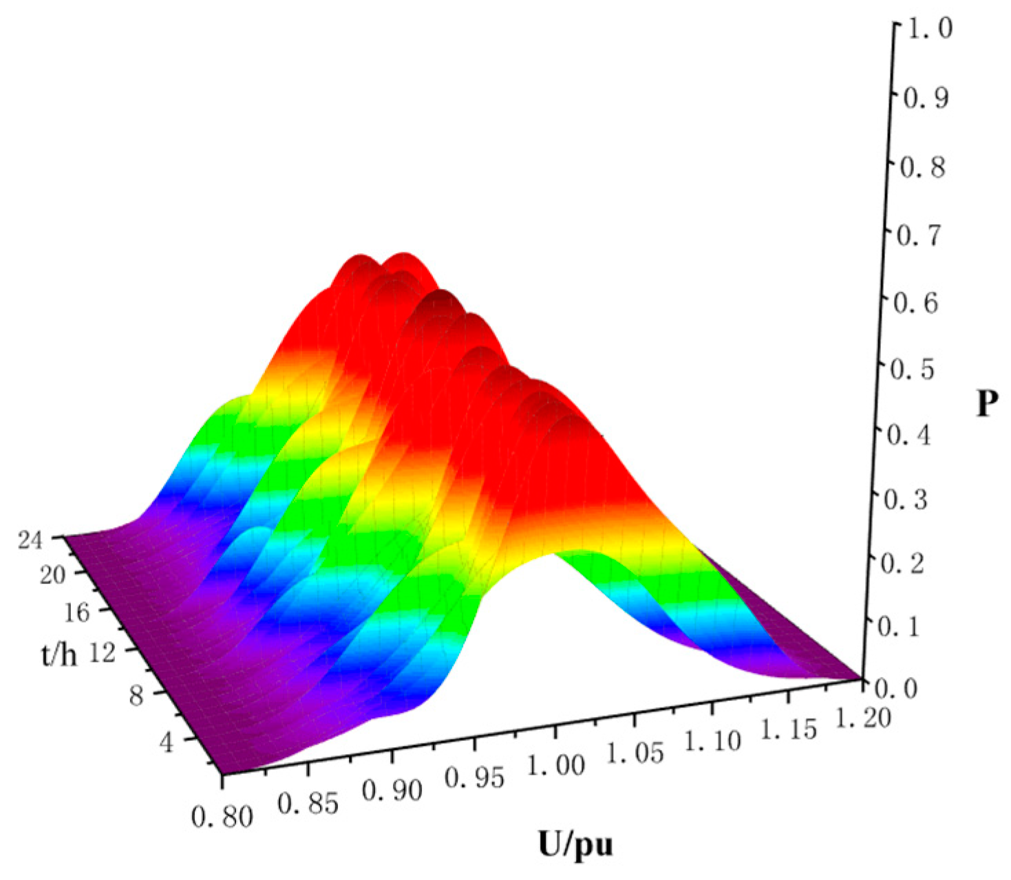
The EV charging power of the 96 intervals is respectively solved by the cumulant method proposed in Section 3.4, and the cumulants of each time interval are added to Node 21. The dynamic voltage PDF at Node 21 with EV uncoordinated charging is shown in Figure 13. According to the dynamic PLF calculation results, the coordinated charging is performed, and the optimized dynamic voltage PDF is obtained, Figure 14:

In Figure 12 with EV integration at Node 21, the PDF of the node voltage amplitude varies greatly with time change, based on the uncoordinated charging scenario. As the EV load is continuously accumulated during daytime, the voltage amplitude corresponding to the extreme point of the PDF is reduced. From 16:00, the power quality deteriorated severely, and the PDF fluctuated significantly, which reaches a peak at 21:00. In addition, during the period from 0:00 to 6:00, the EVs become fully charged, and the charging load is gradually reduced to a minimum value. The voltage amplitude is increased, and the probability density is relatively lowered. With coordinated EV charging, it can be seen from Figure 13 that after the optimization at Node 21, the voltage PDF is apparently stabilized, which alleviates the network pressures.

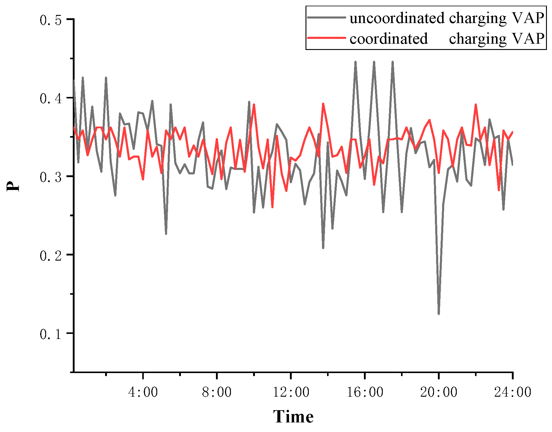
The upper and lower limits of the allowed voltage are −7% and 7%, and the VAP for coordinated charging and uncoordinated charging are calculated according to the data in Figure 12 and Figure 13, as shown in Figure 15. The VDIC index of Node 21 is shown in

Table 7. Node 21 VDIC indicator.

Index	Maximum/%	Minimum Value/%	Mean/%
VDIC	144.612	0.049	15.492

. It can be seen that with coordinated charging optimization, the voltage at Node 21 achieves stable probability fluctuation, which also reduces the risk of the electrical energy network.

5.6. Discussions

Firstly, in Scenario 1 and 2, the simulation results verify the effectiveness, accuracy, speed and feasibility of the proposed PLF algorithm. And then, the results from Scenario 3 show that the wind speed correlation has little effect on the mean value of wind power output and the node voltage amplitude. However, with an increase in wind speed correlation, wind power output and mean square error of the node voltage amplitude will change. In addition, the greater the correlation, the more severe the fluctuation. Finally, Scenario 4 formulates an EV coordinated charging strategy to alleviate grid voltage fluctuation, which can avoid many risks that may occur in the electrical energy network. The research results in this paper are suitable for power system probabilistic stability analysis and optimal power flow.

6. Conclusions

By focusing on the problems of traditional CM based PLF requiring input variables to be independent of one other, and the limitations of Cholesky decomposition for the LHS method, whereby it can only decompose the positive definite matrix, this paper proposes an improved LHS based CM-PLF algorithm using application of the random walk theory. Using realistic case studies based on DG integration, including wind, solar PV and random loads from EV integration into a distribution network, several conclusions are obtained based on four case scenarios.

(1)

The simulation results verify the effectiveness, accuracy, speed, and feasibility of the proposed algorithm. The algorithm can be directly applied to a distribution network with practical DG and EV integration. The algorithm can directly obtain the cumulant of the input variable. The calculation time is extremely short compared with the traditional algorithms, which can provide useful information for the dispatcher and provide effective support for correct decision making.

(2)

This paper analyzes the influence of wind speed correlation. The results show that wind speed correlation has little effect on the mean value of wind power output and node voltage amplitude. However, with an increase in wind speed correlation, wind power output and mean square error of the node voltage amplitude will change, indicating that wind speed correlation can affect the fluctuation of the wind output and node voltage amplitude. Hence, the greater the correlation, the more severe the fluctuation.

(3)

By considering the correlation between DGs and EVs, calculation results are accurate and the other nodes that are without DG or EV integration are influenced little. The inclusion of the spatial correlation coefficient matrix renders greater accuracy.

(4)

With EV integrated into a distribution network, node voltage performance is obviously affected in time domain. Based on the DLF results, this paper formulates an EV coordinated charging strategy to alleviate grid voltage fluctuation, which can avoid many risks that may occur in the electrical energy network.

The ILHS-CM PLF algorithm proposed in this paper is accurate and rapid. The results obtained by this method can be further applied to probabilistic DLF, probabilistic optimal load flow and power system stability analysis. In the future, the research on the PLF algorithm can be combined with the novel sampling method to make the sampling results accurate and inherit the rapidity of the cumulant.