1. Introduction
In recent years, due to the increasingly serious energy crisis and environmental pollution, many countries of the world have vigorously developed new energy sources. As green renewable energy, wind energy has received great attention from countries all over the world. According to the 2018 annual report of the Global Wind Energy Council (GWEC) [
1], the global offshore and onshore installed capacity has reached 23,140 MW and 568,409 MW, respectively. In 2018, the new installed capacity of onshore wind turbines reached 46,820 MW. GWEC expects the onshore market to install upwards of 50 GW per year until 2023. With the increase of the installed capacity of wind power, more urgent requirements are put forward for the daily fault detection and operation and maintenance (O&M) of wind turbines. Due to the remote location of the wind farm, the WTs are exposed to highly variable and harsh weather conditions [
2], which makes the O&M cost of wind turbines higher than other traditional power generation methods. Especially when the wind farm is built at sea, desert, etc., its O&M costs will be much higher. Therefore, it is necessary to vigorously develop wind turbine fault diagnosis technology and to provide early warning of faults and achieve certain accuracy and practicability. Currently, wind turbine manufacturers and research institutes are trying to make breakthroughs in the fault diagnosis and O&M technology of wind turbines.
There are many sensors installed on the turbines to record the working conditions of each component. According to the utility of the data recorded by sensors, the parameter system of the wind turbine can be divided into the supervisory control and data acquisition (SCADA) system, which mainly consists of the performance parameters and the condition-monitoring system (CMS) based on the vibration parameters [
3]. For different fault modes, the parameters such as temperature, power, speed, and blade angle of the turbine will not be the same. Therefore, the relationship between these data and the fault can be explored through machine learning algorithms. SCADA and CMS systems form a big data system for wind turbines. The advantage of big data is that as long as the amount of data is large enough, by selecting appropriate data mining methods and optimizing the data mining process, it is possible to predict unknown parameters and its regularity.
For the fault diagnosis of wind turbines, Professor Andrew Kusiak of the Intelligent Systems Laboratory of the University of Iowa has made great achievements. Kusiak et al. [
4] developed virtual models of a wind turbine which were extracted by six machine learning algorithms. The power output and rotor speed were selected as performance parameters to test the proposed methodology. In [
5], a three-level fault prediction methodology based on the SCADA data and status data of 4 wind turbines was proposed. In order to predict the blade angle asymmetry and implausibility faults, an association rule mining algorithm was applied and five classifiers were used to identify the best model [
6]. Also, the bearing faults were analyzed by building a normal behavior model based on the neural network algorithms in [
7]. The test results on five over-temperature events validated its effectiveness on bearing faults prediction.
Generally speaking, the approaches for wind turbine fault detection/prediction through data mining algorithms are divided into two major ways. One is through normal behavior modeling (NBM) [
8]. By selecting the historical SCADA data under normal conditions as the training set, the normal behavior model of the key components of the turbines can be constructed. Support Vector Machine (SVM) [
9,
10], neural network [
11], and deep belief networks [
12] are commonly used algorithms in NBM. Then, according to the statistical characteristics of the normal conditions of the wind turbine, an empirical threshold is set as an alarm line so that any fault deviates from the normal conditions can be detected. Bangalore et al. [
13] constructed an artificial neural network (ANN) normal behavior model to predict the gearbox fault. During the anomaly detection stage, a Mahalanobis Distance (MHD) method was presented to describe the deviation between the ANN model and the operating condition. Finally, the case studies of four wind turbines illustrated the effectiveness of the proposed approach. For other subcomponents of the turbines, such as the generator bearings and slip rings, etc., the evolution of their faults develops faster than that of gearbox and thus it is difficult to make timely intervention before the fault occurs. Therefore, it is particularly important to achieve the fault prediction of these subcomponents through advanced analysis techniques. In [
14], a nonlinear state estimate technique (NSET) is proposed to construct the normal behavior model of the generator temperature. In [
15], the selected model is principal component regression and can identify the incoming generator slip ring fault approximately one day in advance. In [
16], the authors proposed a model-based approach to predict generator bearing temperature and thus achieving the early detection of bearing and gearbox faults.
The other way is a classification-based approach. The classification-based approach is to divide the operating state of the wind turbine into different categories (label), such as normal operation, shutdown, or a specific type of fault. Each sample in the training set consisting of SCADA historical data has a label. Then the classifier after the training process can be used to determine the type of fault of the turbines. Association rule is a commonly used algorithm. The authors in [
6] used the Apriori algorithm to identify the correlation from the database composed of fault categories, various operating parameters, and history records and then identified the specific fault mode. Similarly, in [
17], the Apriori algorithm was applied to find the key event codes of wind turbines.
For the NBM approach, no matter which algorithm is used to establish the prediction model, most of the approaches during the fault prediction stage are achieved by analyzing the residual and setting a single alarm threshold. The authors in [
18] used the Mahalanobis distance instead of the residual and applied the Weibull distribution to obtain the threshold of the fault alarm. Wu et al. [
19] developed a normal behavior model for wind turbines gearboxes using echo state networks. The potential faults were detected through residual evaluation and dynamic threshold setting. However, using a single alarm threshold or an adaptive threshold method often has a time uncertainty problem, that is, an accurate time point at which the fault symptom begins to appear cannot be given. Moreover, an inappropriate threshold setting may cause a false alarm or miss detection, which makes the fault prediction based on SCADA data has the problems of low prediction accuracy and low computational efficiency. In order to improve the reliability and accuracy of fault prediction, we propose a gearbox fault prediction approach based on a stacking model and CUSUM (Cumulative Sum) control chart. The framework of the proposed method can be divided into four parts, which are the data preprocessing, feature selection, the normal behavior modeling process, and the fault prediction process, where several algorithms or their combinations were applied. The main contributions of our work and the functionality of these algorithms are summarized as follows:
During the data preprocessing process, we select the SCADA historical data under the normal working conditions and apply the Density Based Spatial Clustering of Applications with Noise (DBSCAN) algorithm and the quartile method to recognize and filter out the three types of outliers and abnormal data. The DBSCAN algorithm plays an important part in filtering out most of the outliers and then the quartile method is applied for further preprocessing to improve the data quality.
During the feature selection process, three data mining algorithms are used to select the features most relevant to the gearbox oil temperature as the input variables of the model.
Based on the Stacking idea, a normal behavior model including Random Forest (RF), GBDT, and XGBOOST is established to describe the temperature characteristics of the gearbox under normal operation state. By comparing the performance of seven single models on three metrics, we finally select three models, RF, GBDT, XGBOOST, as the basic models of our proposed stacking model. The proposed stacking model trains three basic models in parallel which can avoid the defect of a single machine learning model like overfitting and low prediction accuracy. The case study illustrates the superiority and effectiveness of the proposed model.
The change-point detection algorithm based on CUSUM control chart is applied to detect the change points in the MD series. Compared with the fault detection algorithm by setting a single threshold, the proposed approach can accurately locate the time at which the fault symptom begins to appear. A case study on five faulty turbines shows the proposed approach can predict the faults 13 to 22 days in advance.
The rest of this paper is organized as follows:
Section 2 briefly introduces three types of abnormal data and illustrates the necessity of data preprocessing.
Section 3 clarifies the structure of the proposed approach.
Section 4 introduces the data set used in this work and the entire process of normal behavior modeling. In
Section 5, we use the data of five turbines to test the performance of our proposed approach and list the test results.
Section 6 summarizes the full paper and points out the future research direction.
2. Background Review
The complete wind turbine consists of the gearbox system, generator system, pitch system, yaw system and other key components [
20]. The gearbox is an important component of the wind turbine transmission system. Its main function is to transmit the power generated by the blade under the action of the wind to the generator and achieve a higher speed. At present, the gearbox manufacturing technology is relatively mature and has high reliability, however, due to its frequent high-speed, heavy-duty, and high-impact working environment, it is prone to suffer various faults within an operational period of 5 years, and has to be replaced [
21]. Moreover, the system shutdown caused by gearbox failure takes the longest time and a gearbox replacement can cost up to 14.5 percent of the wind turbine maintenance cost [
20]. Therefore, gearbox fault prediction is necessary.
Generally, gearbox faults can be reflected by the change of gearbox oil temperature. In [
22], the authors illustrated that the rise of oil temperature could indicate the development of the gearbox faults. And an artificial neural network model was constructed to predict the oil temperature. In this work, the gearbox oil temperature is modeled to describe the working status of the wind turbine.
The normal behavior modeling approach has high requirements for the quality of training data: fault-free SCADA data must be accurately selected [
23]. However, due to sensors’ accuracy degradation, communication failure, and curtailment, the turbine can operate in different modes even under normal conditions [
24].
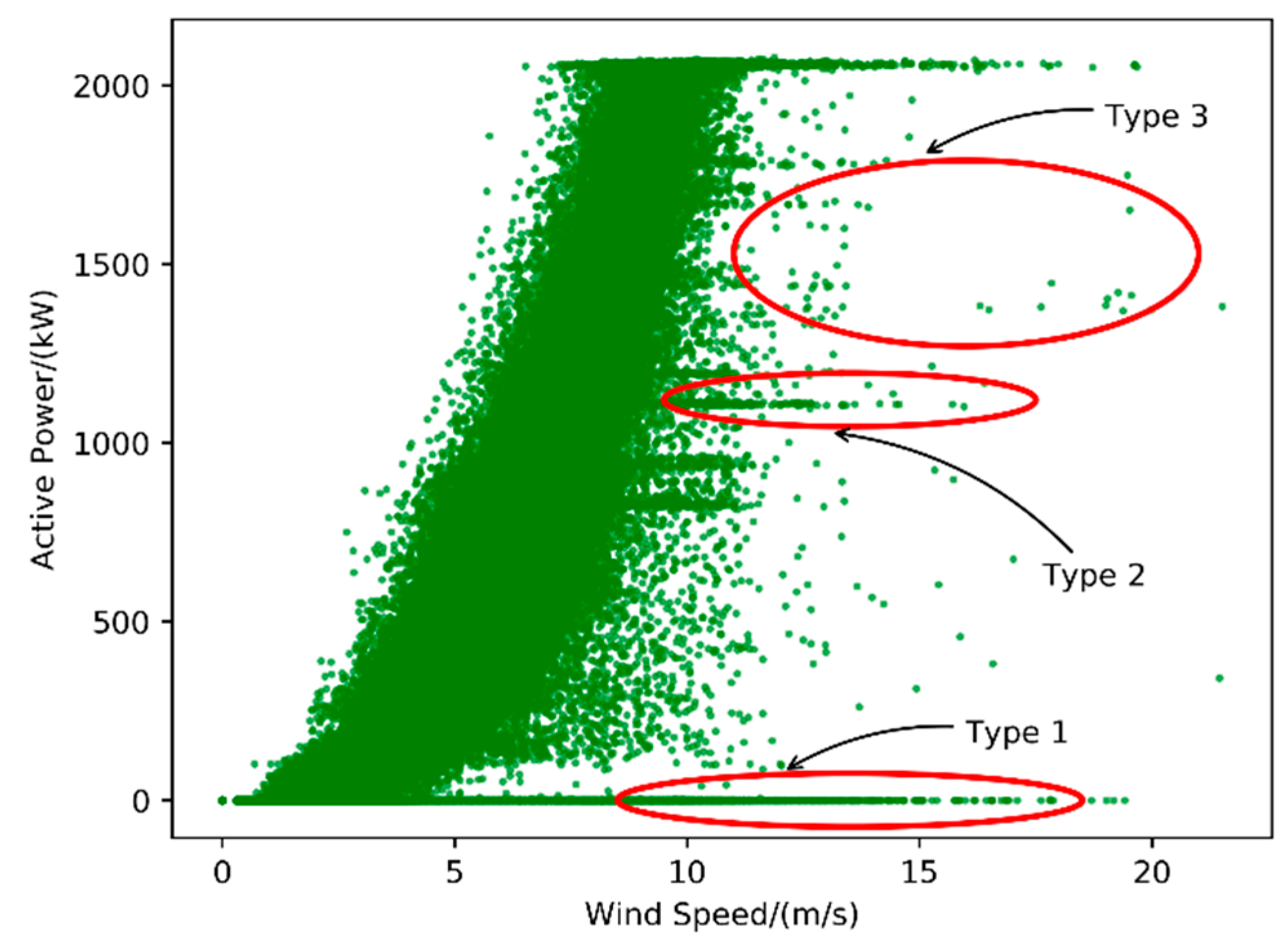
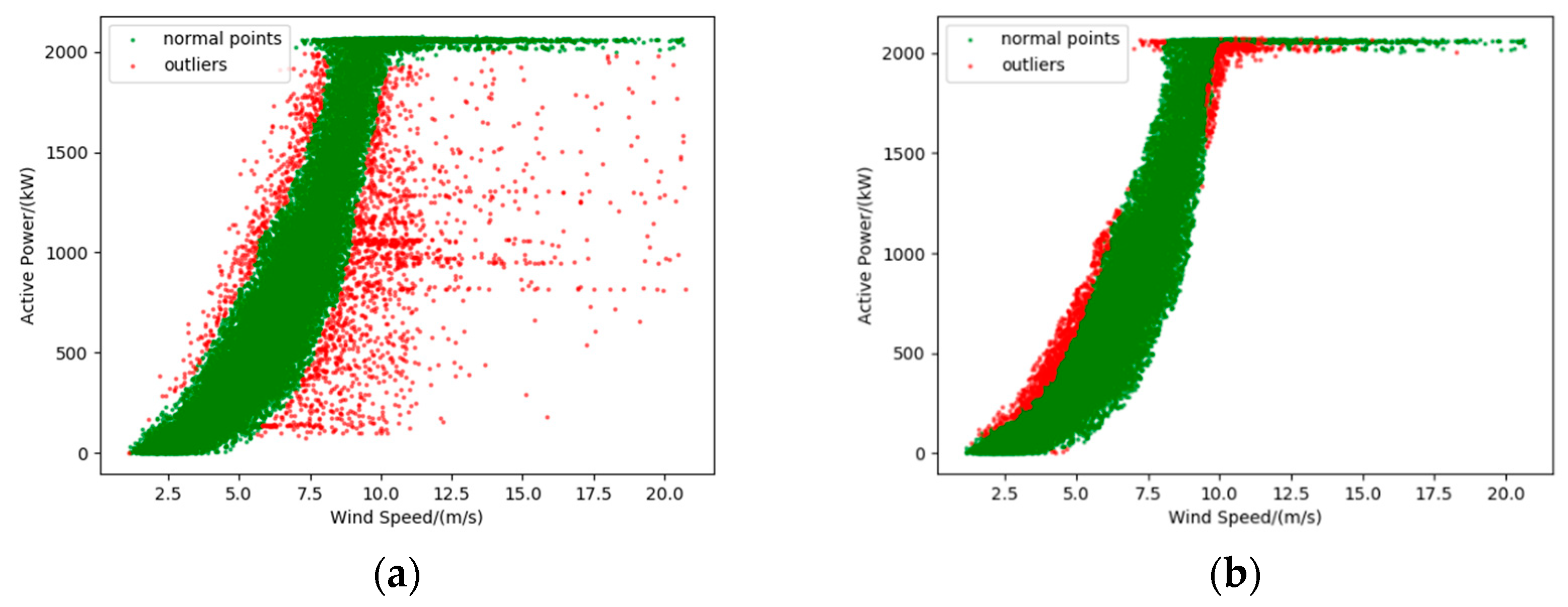
Figure 1 shows three common types of anomaly data in the power curve:
The lower stacked abnormal data is represented as a horizontally dense data cluster in the scatter plot, as shown in Type 1 in
Figure 1. Type 1 indicates the points where the wind power output from the wind turbine is 0 regardless of the wind speed. Such abnormal data appears due to damage to the power measuring instrument or abnormal communication equipment, fault of the wind turbine, etc. [
25].
Wind curtailment data. The “Wind curtailment” data appears as a horizontally dense cluster of data in the scatter plot, typically in the middle of the curve, as shown in Type 2 in
Figure 1. Such anomaly data shows that the output power of the wind turbine does not change with the change of wind speed. Wind curtailment is the reduction in electricity generation below what a system of well-functioning wind turbines are capable of producing [
26], which is usually enforced by wind farms. The following are the main causes of “Wind curtailment”. First, China’s energy structure is still dominated by thermal power generation, supplemented by new energy, so wind power generation is only used as regulating power. Second, because of the excess capacity of wind power, it is difficult to store large capacity wind power resources, so it is necessary to curtail wind power. Finally, due to the instability of wind speed, the electric energy generated by the wind turbine is also unstable. When the wind speed has a huge fluctuation, the grid-connected cannot be performed forcibly, so the wind curtailment operation has to be carried out at this time.
The dispersive anomaly data is randomly distributed around the curve, as shown in Type 3 in
Figure 1. The distribution of such anomaly data is irregular and is usually caused by sensor accuracy degradation, instrument fault, or noise during the signal propagation.
If these raw SCADA data are directly used for analysis and modeling, it will inevitably lead to a decrease in prediction accuracy and difficulty in achieving research goals. Therefore, it is necessary to preprocess the raw data collected by the SCADA system before establishing the normal behavior model.
3. Framework for Proposed Fault Prediction Approach
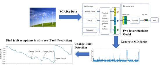
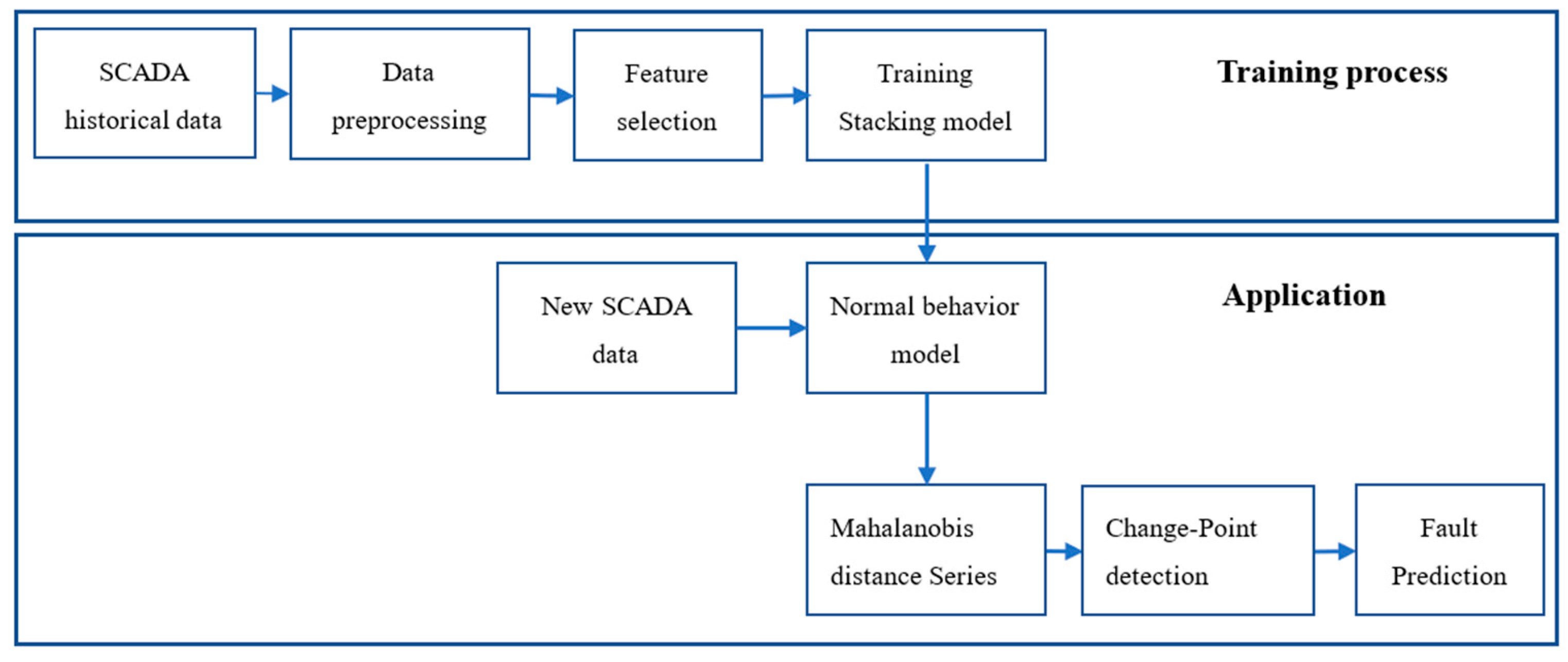
The main idea of our proposed fault prediction approach is to fit the normal operating behavior of wind turbines by establishing a normal behavior model of the gearbox oil temperature, and then use the Mahalanobis distance, instead of the residual, to describe the deviation between the actual measured value and the model output value. Finally, the Change-point detection based on CUSUM control charts is applied to implement the gearbox fault prediction. The overall flowchart of the fault prediction model proposed in this study can be divided into the training process and application process, as shown in
Figure 2. The training process deals with the necessary data preprocessing and feature selection, which are performed based on the historical data collected by the SCADA system to establish the normal behavior model of the gearbox. During the application process, the real-time SCADA data is input into the normal behavior model after the same data preprocessing and feature selection. There is a certain deviation between the predicted values of the model and the actual values recorded by the SCADA system. The larger the deviation is, the higher the possibility of a fault happens. In this work, we apply the Mahalanobis distance to describe this deviation. By inputting the Mahalanobis distance series into the proposed Change-point detection algorithm, the time at which the fault occurs and the time at which the fault symptom begins to appear can be obtained, and thus the fault prediction can be realized.
3.1. Data Preprocessing
From
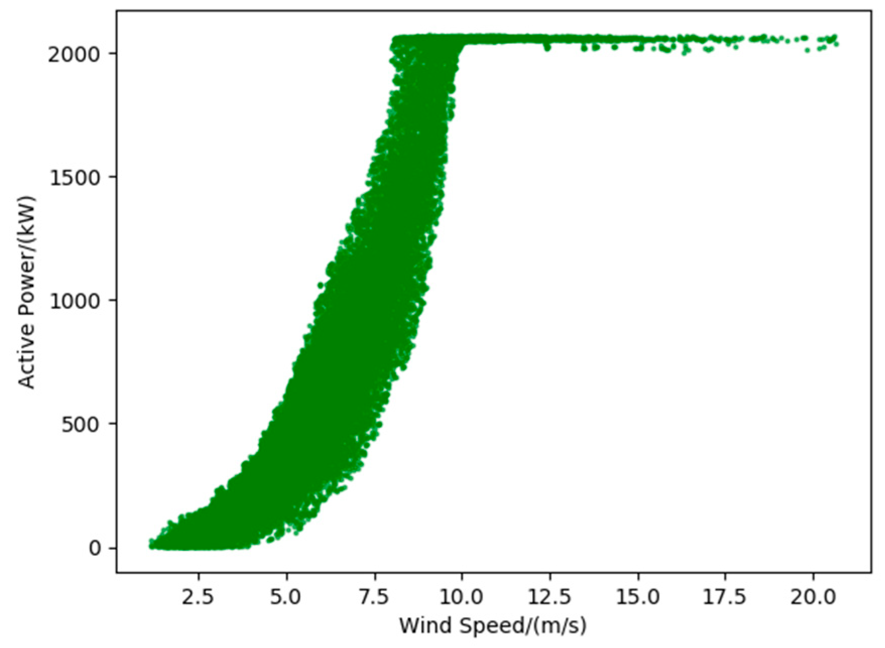
Figure 1, we can see intuitively that the three types of anomaly data points show obvious outlier characteristics in the power curve. In this work, we apply the combination of DBSCAN and the quartile method to identify the anomaly points and outliers. The case study of wind turbines using SCADA data has validated this data cleaning method, which demonstrates its effectiveness and generality.
DBSCAN is a typical density-based clustering algorithm, which is designed to discover the clusters and the noise in a spatial database [
27]. According to two input parameters, Eps and MinPts, the algorithm divides the data to be clustered into three categories: core points, border points, and noise points. A core point refers to the point in a cluster that there are at least a minimum number of points in an Eps-neighborhood of that point. The Eps-neighborhood of border points contains fewer points than core points. And the points not belong to core points or border points are defined as outliers (noise), which are the anomaly data to be filtered in this work. Compared with the K-Means clustering algorithm, the DBSCAN does not need to determine the number of cluster centers in advance and can identify clusters of arbitrary shapes and has strong anti-noise ability.
The quartiles are a type of quantile which can be applied to check for outliers [
28]. In this work, we used the first quartile (
Q1) and the third quartile (
Q3) to achieve the further preprocessing of the data after the DBSCAN method. The first quartile refers to the middle number between the smallest number and the median of the data set. The third quartile is defined as the middle value between the median and the highest value of the data set. By calculating the
Q1 and
Q3, we can get the interquartile range (
) which defined as follows:
According to the
IQR, we can get the normal data bounds expressed as follows:
where
Fl and
Fu are the lower limit and upper limit of normal data, respectively. Any data lying outside the defined bound can be considered an outlier. In this work, the quartile method is adopted by dividing the wind speed data into different intervals and then to filter the active power data in each interval correspondingly. The interquartile range is the same as the variance and standard deviation, which can represent the dispersion of statistical data of a variable. But the interquartile range is relatively robust statistics since the value of
IQR does not change significantly with individual abnormal data. However, this method has its limitations, that is, the method can correctly and effectively identify these abnormal data only when the proportion of abnormal data to the total amount of data is small.
Hence, in this study, the combination of the DBSCAN and quartile method is applied for data preprocessing. It can be seen from
Figure 1 that the proportion of three kinds of abnormal data is relatively large. If we user the quartile method directly, the abnormal data is bound to affect the value of the
IQR. Moreover, the density of these abnormal data is significantly less than normal data. Therefore, in the data preprocessing stage, the DBSCAN is firstly used to identify and remove most of the abnormal data, the SCADA data is further processed by the quartile method to improve the quality of data cleaning.
3.2. Feature Selection
Feature selection is a significant part of the data mining process. As the input of the model, features determine the quality of the model. Generally, feature selection is executed by selecting a subset from many features or applying a suitable method to reduce the dimension. The purpose of feature selection is to remove redundancy, reduce the number of features, improve model accuracy and reduce run time. In this work, to establish the normal behavior model of the wind turbine gearbox, the gearbox oil temperature is selected as the output variable. Three feature selection algorithms, namely, filter model [
29], wrapper model with recursive feature elimination (RFE) algorithm [
30,
31], and RF model [
32,
33], are applied to select the features most relevant to the gearbox oil temperature as the input variables of the model. These three algorithms are typical feature selection methods based on how to generate feature subsets [
34]. They will calculate the most relevant features according to different rules, which can avoid the defect of a single method. By inputting the SCADA data with whole 39 parameters as input variables, we obtained the top 10 most relevant parameters ranked by each algorithm and finally choose 15 parameters as the input variables.
3.3. The Stacking Model
The oil temperature of the gearbox is affected by many factors including the working condition and the inherent properties of wind turbines, thus making the status information complicated. To avoid the defects of the single model, we propose a model based on the Stacking strategy by combining three regressors for temperature predictions. At present, the machine learning model based on the stacking strategy has been widely applied in Kaggle competition, sentiment classification [
35], speech recognition [
36], and many other application scenarios. As far as we know, there are still no researchers who have applied stacking strategy to wind turbine fault prediction.
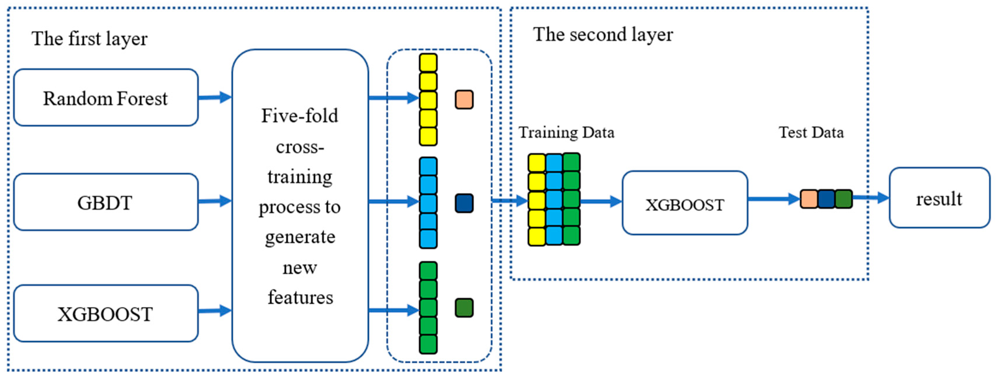
In this work, a two-layer stacking model is proposed to construct the normal behavior model of gearbox oil temperature as shown in
Figure 3.
The first layer consists of three basic models, including RF [
32], GBDT [
37], and XGBOOST [
38]. The idea of stacking is to train these basic models in parallel and combine them by training a meta-model to output predictions based on the multiple predictions returned by these basic models [
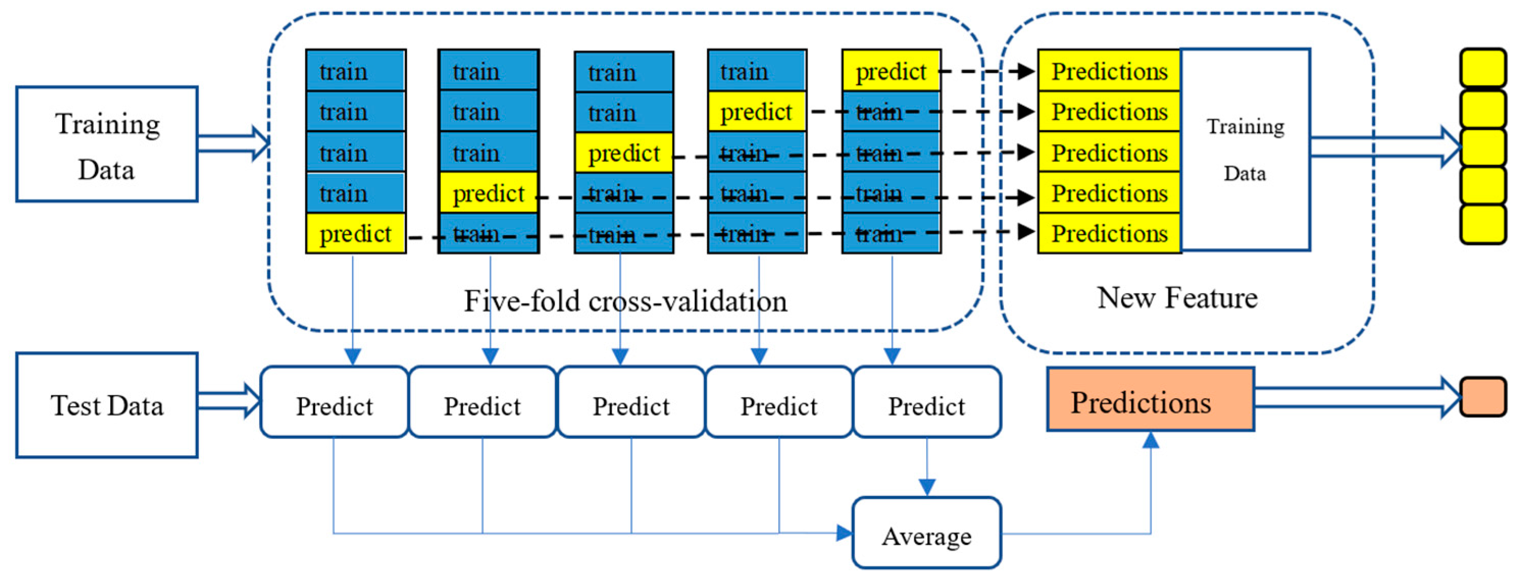
39]. For each basic model, we use five-fold cross-training, which is similar to k-fold cross-validation, to generate training data and test data for the meta-model in the second layer.
Figure 4 describes the details of this process.
The training data is divided into five folds. In each training process, four folds are used for training and the remaining one fold is used for making predictions for observations. In other words, the five-fold cross-training consists in training on four folds in order to make predictions on the remaining fold and that iteratively so that to obtain predictions for observations in any folds. By combining these predictions of three basic models as new features, we can obtain the training data of the meta-model in the second layer. Other than this, each basic model can produce five predictions of the original test data. We take the average of these predictions as the test data for the meta-model. In the second layer, with the training data and the test data produced by the cross-training process, the XGBOOST model is trained as the meta-model and output the final predictions based on the test data.
The proposed stacking model acts as a normal behavior model to generate a prediction of the gearbox oil temperature based on the given input features. In this work, by inputting the 15 features we selected, the stacking model will output the prediction of gearbox oil temperature at this time. Its superiority lies in the part that it can train three single machine learning models in parallel, which greatly accelerates the training process. The performance of our stacking model on the test data has validated its effectiveness.
3.4. Fault Prediction Approach
3.4.1. Mahalanobis Distance Series
The Mahalanobis distance is an effective method for calculating the similarity of two unknown sample sets. Compared to the Euclidean distance, the MD is scale-invariant and takes into account the correlations of the data set. At present, the MD has been introduced into the field of wind turbine fault detection to determine the fault alarm threshold [
12,
13]. In this work, we use the MD to quantify the deviation between the test data (real-time SCADA data) and the normal behavior model. The MD for the normal behavior model can be expressed as follows:
where
.
MVi represents the
i-th measured value recorded by the SCADA system during the five-fold cross-validation process and
erri is the validation error;
Cnor and
μnor are the covariance matrix and the mean value vector of
Xnor;
is the Mahalanobis distance of the vector
.
During the fault prediction stage, we input the real-time SCADA data into the normal behavior model and calculate the corresponding MD series as the input of the subsequent change- point detection algorithm. The MD in this stage is defined as follows:
where
is consists of the test error
erri and the measured value
MVi during the fault prediction stage;
Cnor and
μnor are the covariance matrix and the mean value vector obtained from the normal behavior model. l;
is the final MD series as the input of the change-point detection algorithm.
3.4.2. Change-Point Detection
At present, most of the fault detection approaches of wind turbines analyze the residual series by setting the single threshold or adaptive alarm threshold, which has the problem of time uncertainty. In this work, we applied the change-point detection algorithm based on the CUSUM control chart to analyze the MD series.
The CUSUM control chart is drawn by the cumulative sum of the difference between the observed value and the target value. It is widely used in the field of economics because of its simple and intuitive characteristics. If the statistical value is higher than the average value over a period of time, this amount of data will continue to accumulate, and the CUSUM control chart will show a steady growth trend and vice versa. Therefore, the CUSUM control chart can detect whether there is a change in the series, but the detailed information of the change point, such as confidence level and confidence interval, cannot be obtained only through the control chart [
40]. Therefore, in this work, we propose a fault prediction algorithm combining the CUSUM control chart and change-point detection, which can accurately capture the small abnormal changes in the MD series. Algorithm 1 below describes the calculation process of the algorithm.
| Algorithm 1: Change-Point Detection. |
| Data: Mahalanobis Distance Series MD and its length M; Confidence Level C; Number of bootstrap samples performed N |
| Result: index of the change point |
| 1 | Calculate the average |
| 2 | Calculate the cumulative sums by adding the difference between the current value and the average to the previous sum. for i = 1, 2, …, M and S0 = 0 |
| 3 | Calculate the original Sdiff which defined as: Sdiff = Smax − Smin—where , |
| 4 | for j in range (1, N) do |
| 5 | Generate a bootstrap sample of the original MD series, denoted |
| 6 | Based on the bootstrap sample, calculate the bootstrap CUSUM, denoted |
| 7 | Calculate the difference of the bootstrap CUSUM, denoted |
| 8 | Compare each with the original Sdiff, let X be the number of bootstraps for which for j = 1, 2, …, N |
| 9 | Calculate the confidence level P that a change occurred as a percentage: and compare with the input confidence level C |
| 10 | If P > C, a change has occurred with a confidence level of C |
| 11 | Output the index of the change point m, let m be such that: |
The input parameters of the algorithms are the MD series, its length and set a confidence level C and the number of bootstrap samples performed N. The functionality of the proposed approach is to find the possible change point in the MD series obtained from our normal behavior model and then output the index of the change point with the given confidence level. In other words, the change point output by our algorithm is calculated by a large number of repeated sampling and obtained based on the probability. Our fault detection approach will perform bootstrap sampling N times on the original MD series and will generate a new random sorted MD series each time. If the majority of the new series are recognized as having change points, we are confident about the conclusion that there exist change points in the original MD series. For example, if the algorithm finds that there are 900 new MD series containing change points in the total 1000 times of bootstrap sampling, we can draw a conclusion that the original MD series have change points with a confidence level of 90%. The final number of change points depends on the confidence level we set. If we set a relatively low confidence level, there is a high possibility that we will get many change points, which including the points at which the real fault happened as well as the points turn out to be unreliable. To get more reliable results, we can set a higher confidence level so that we will much more confident about the change points obtained from our algorithms and they will be closer to the real conditions.
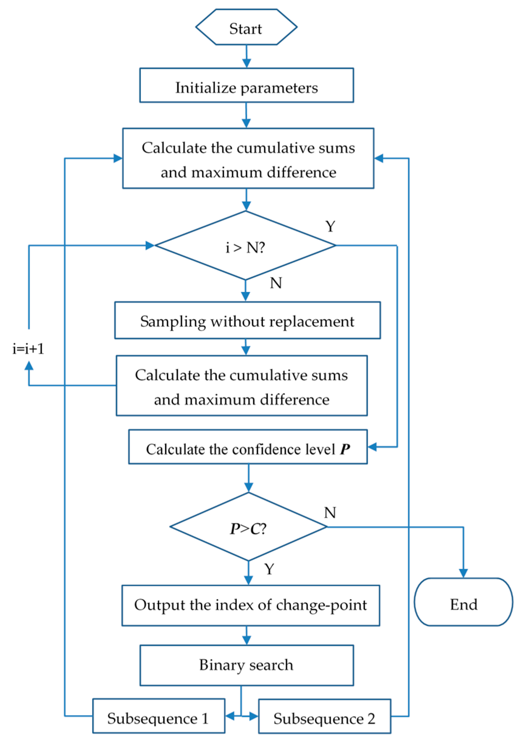
The principle of using the CUSUM control chart to judge whether a change has taken place in the series is to generate new MD series by multiple sampling without replacement. If the maximum difference of the cumulative sum of the new series is mostly smaller than that of the original series, we have reason to believe that a change must have occurred in the original MD series. The more this happens in N times sampling, the higher the confidence level of a change happens. Once a change has been detected, it is also necessary to determine when the change occurred. In this work, we use the binary search algorithm to specify the index of the change point. The original MD series is divided into two parts based on the change point found by the change-point detection algorithm, similar to the binary search algorithm, we iteratively execute the Algorithm 1 on each subseries until all the change points that satisfy the confidence level are accurately found.
Figure 5 is the flowchart of the entire change-point detection process.
5. Testing Fault Prediction Approach
In this section, the proposed approach has been applied in five wind turbines (two turbines of type A and three turbines of type B) to predict the gearbox fault. According to the fault alarm record of the wind farm, the five turbines have suffered gearbox oil temperature over-limit fault during the selected time period. First, the test data is input into the normal behavior model we established to obtain the MD series on the test data set. Then, the change-point detection algorithm is applied to analysis the MD series, and the time point at which the fault occurs and the time point at which the fault symptom begins to appear can be obtained to achieve the fault prediction. In this work, the time interval of the MD series is 5 min, the number of sampling is set to 1000, and the confidence level is 0.99 and 0.90 respectively. The test results of the fault prediction algorithm are as follows.
5.1. Test Results for Turbine #38
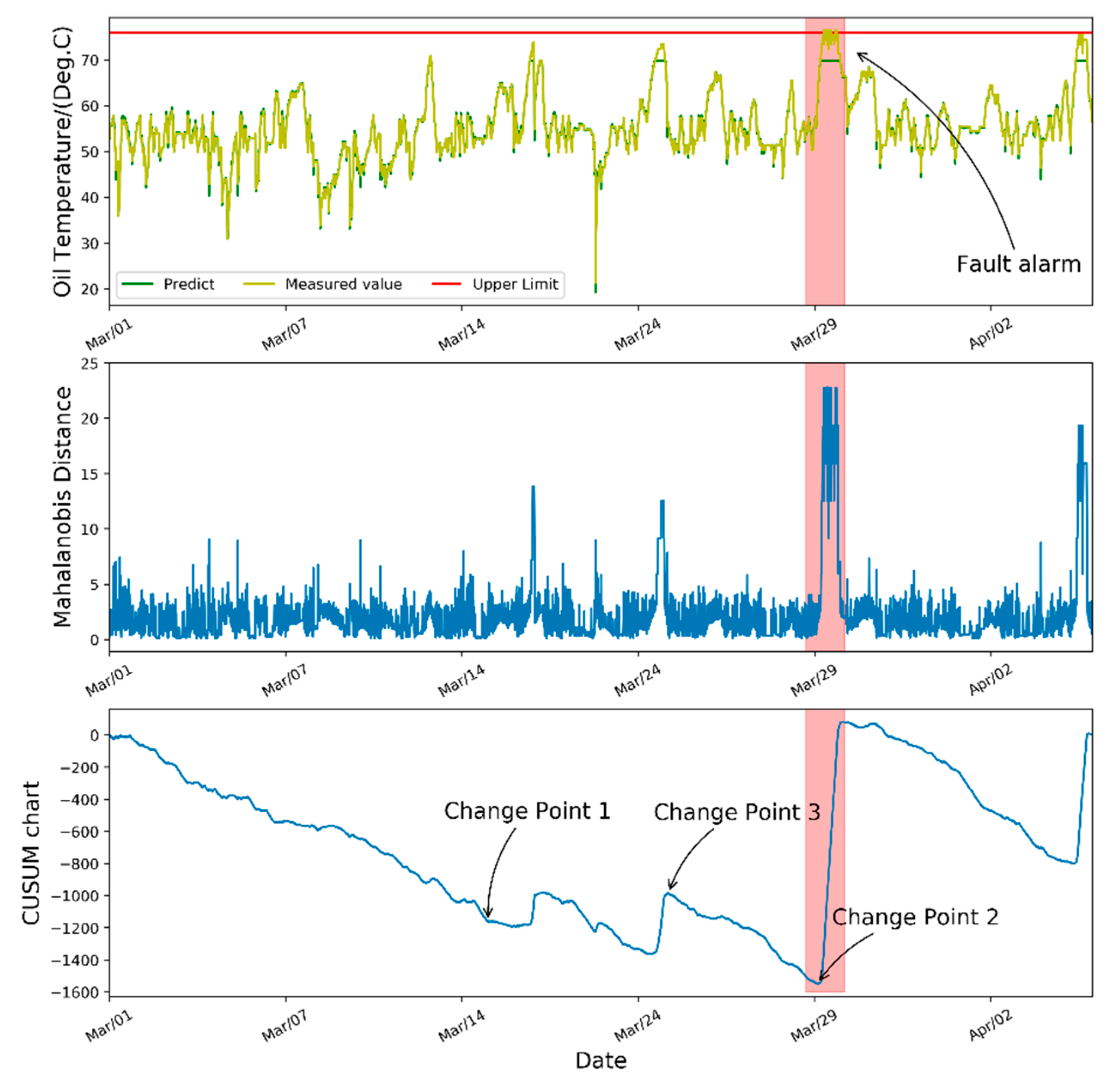
Figure 10 displays the fault prediction results of turbine #38, which consists of the gearbox oil temperature curve, MD series, and CUSUM control chart in turn. There are two change points detected by the change-point detection algorithm which were marked in the figure. The change point 1 indicates that the fault symptom begins to appear at 11:42 on 15 March 2018, which is the 2148th sample point. The change point 2 indicates the actual fault that happened at 11:24 on 29 March 2018, which is the 4015th sample point calculated by our algorithm. It can be seen from the temperature curve the measured value has exceeded the upper limit at the corresponding time of change point 2, at which the MD value also has a drastic increase.
From
Table 6, it is worth noting that the confidence level of change point 3 is 0.90, which means we only get two change points under the confidence level of 0.99. The confidence level indicates how confident the result is that the fault actually occurs or the fault symptom begins to appear. The change point 1 occurred with 99% confidence. While the change point 3 occurred with 90% confidence. That means in the 1000 times of bootstrap sampling, the change point 3 was detected at least 900 times while the change point 1 and 2 were detected at least 990 times. Therefore, we are much more confident about the change point 1 at which the fault symptoms begin to appear.
According to the fault alarm record of the wind farm, the gearbox oil temperature over-limit fault did happen at 15:10 on 29 March 2018, which is almost consistent with the time point 2 calculated by the change point detection algorithm. Although the gearbox oil temperature at change point 3 is close to the upper alarm limit, no gearbox fault has occurred. Thus, change point 3 is only a potential change point with a low confidence level. Therefore, we can achieve the fault prediction by sending out an alarm signal at the time of change point 1 to arrange the operation and maintenance work. The case study preliminarily verifies the effectiveness of our fault prediction algorithm to recognize the fault symptoms, and thus send out the alarm signal 14 days in advance. Other than this, the proposed change point algorithm can generate different results based on the confidence level we set. Generally speaking, the lower the confidence level we set, the more change points been recognized. But quite low confidence levels will lead to an unreliable result like a false alarm.
5.2. Test results for Turbine #173
Similarly,
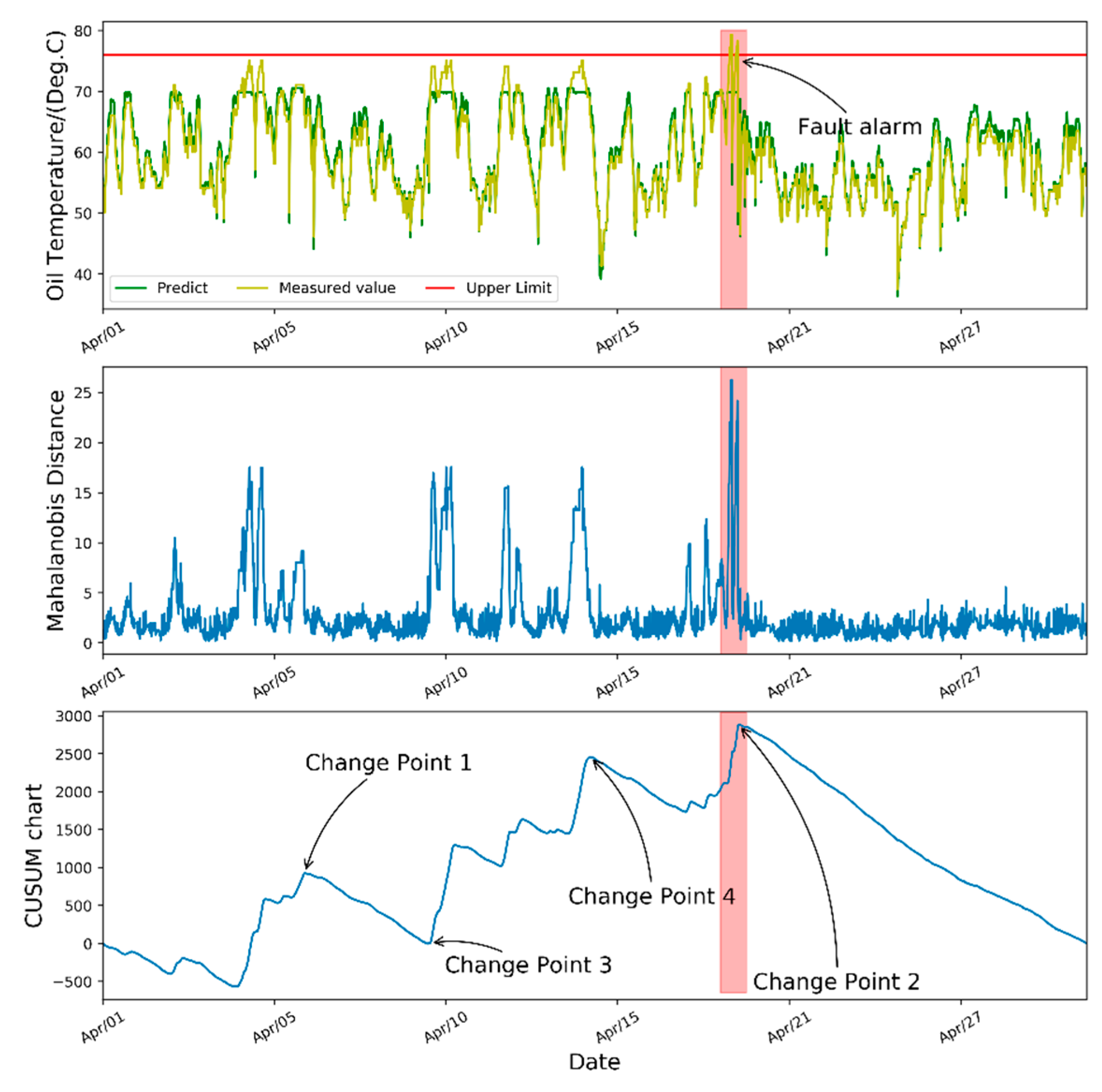
Figure 11 shows the fault prediction results of turbine #173. The fault symptom begins to appear at 03:24 on 6 April 2018, with corresponding to the change point 1. The change point 2 indicates the fault finally happened at 08:32 on 19 April 2018.
Table 7 lists the information about the four change points. When the confidence level is reduced from 0.99 to 0.90, in addition to the original change point 1 and 2, the algorithm also detects the change point 3 and 4. However, there is no fault happened at the timestamp corresponding to change point 3 and 4.
According to the fault alarm record, turbine #173 had a temperature over-limit fault at 06:52 on 19 April 2018. We are much more confident about the change point 1 at which the fault symptoms beginning to appear. Therefore, the fault prediction algorithm can detect the fault 13 days in advance. Through the analysis of the above two turbines, we can find that the proposed algorithm can not only identify the time of the fault happens but also accurately detect the time point at which the fault symptom begins to appear with a certain confidence level so as to realize the fault prediction.
5.3. Test Results for Other Turbines
The proposed algorithm was applied to the other three wind turbines to prediction the gearbox fault. All these three turbines have suffered gearbox oil temperature faults during the selected time period.
Table 8 lists the test results. It can be seen from the figure that the faults can be detected 16 to 22 days in advance. The difference in prediction results may be related to the type of wind turbines and the severity of the fault.
6. Conclusions
In this work, a gearbox fault prediction approach has been proposed by building a normal behavior model and analyzing the MD series through the change-point detection algorithm. During the modeling process, a data cleaning method composed of the DBSCAN and quartile was applied to identify and drop out the anomaly data. Then, two stacking models were constructed for each type of wind turbines by inputting 15 features to describe the gearbox oil temperature under normal conditions. Compared with other single models, the stacking model can achieve better performance on three metrics and can also overcome the defects of the single model, such as the over-fitting problem.
The effectiveness of the proposed approach was verified using the SCADA data of a wind farm in Ningxia, China. Considering that there are a large number of wind turbines in the wind farm, we use the SCADA data of five turbines for half a year period to establish the normal behavior model of the turbines, so that the model can be used for fault prediction of all other turbines of the same type without separately building models for each turbine. Finally, we verified the fault prediction algorithm on two normal turbines and five fault turbines. The case study shows that the algorithm can detect the fault symptoms 13 to 22 days in advance.
The proposed approach in this paper mainly has two aspects. The Mahalanobis distance, on the one hand, is applied to quantify the discrepancy between the model output value and the actual value of oil temperature. It can be seen from the MD figures that the series of turbines under normal conditions is relatively stable and there is no large fluctuation. Contrary to this, the MD value of the faulty turbines will have a drastic increase when the fault happens, which proves its rationality of using MD to measure the deviation between the actual and normal conditions of turbines. On the other hand, the change-point detection algorithm can not only identify the time point at which the fault occurs, but more importantly, it can detect the time point at which the fault symptom begins to appear, thereby scheduling the operation and maintenance work in advance, and realizing the fault prediction.
In conclusion, we have proposed a fault prediction approach based on a stacking model and change-point detection. The stacking model, as the normal behavior model to describe the normal conditions of wind turbines, its prediction accuracy is obviously higher than that of other single models and is especially suitable for dealing with the occasions with a large amount of data and complex parameter relationships in wind farm. The stacking model can also be applied to power forecasting and the power optimization of wind farms. In addition, compared to the traditional fault detection approach by setting an alarm threshold, our approach is capable of providing more information on the incoming fault. It can not only determine the time at which the fault symptoms beginning to appear, for each change point, it also provides further information including a confidence level representing the possibility that a fault symptom is about to appear. The higher the confidence level is, the more we are confident about the fault prediction result. During the actual application stage, by setting a proper confidence level in advance, the personnel of the wind farm can arrange the operation and maintenance work at the corresponding time of the change point detected by the algorithm, repairing the gearbox in advance, and achieving the goal of fault prediction.
It is worth noting that, unlike setting a single threshold for fault detection, we use the method of change-point detection for the MD series to predict the fault. However, due to the inherent limitations of the change-point detection algorithm itself and the complicated state of the turbines during actual operation, it is also possible to detect the existence of change points in the MD series of a normal turbine, which may lead to a false alarm. In this case, it is of vital importance to select the proper test interval during the actual application stage. For example, in this paper, we use the SCADA data for a period of a month for fault prediction. That is to say, the length of the MD series can significantly affect the accuracy of the final detection result. Take
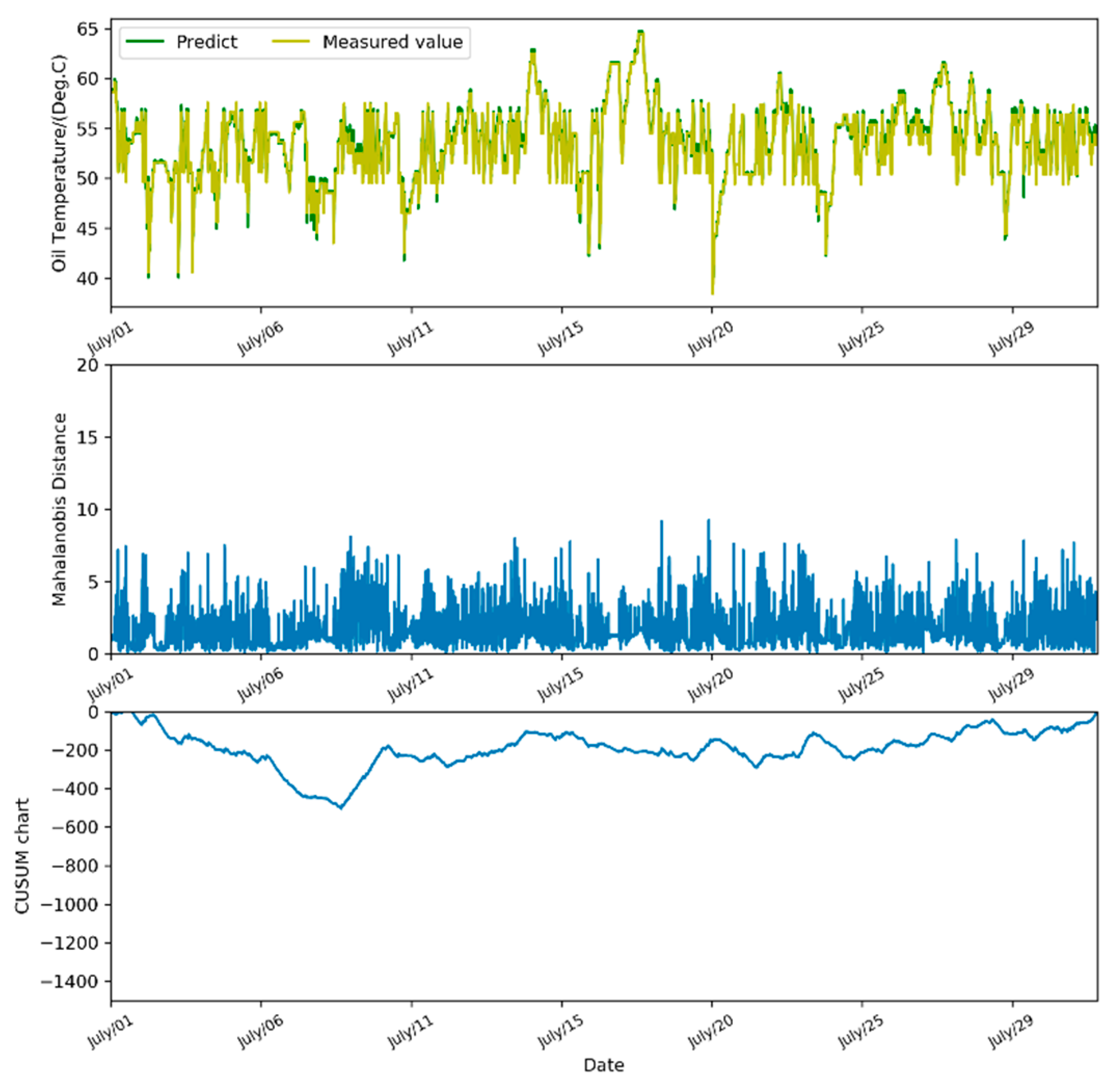
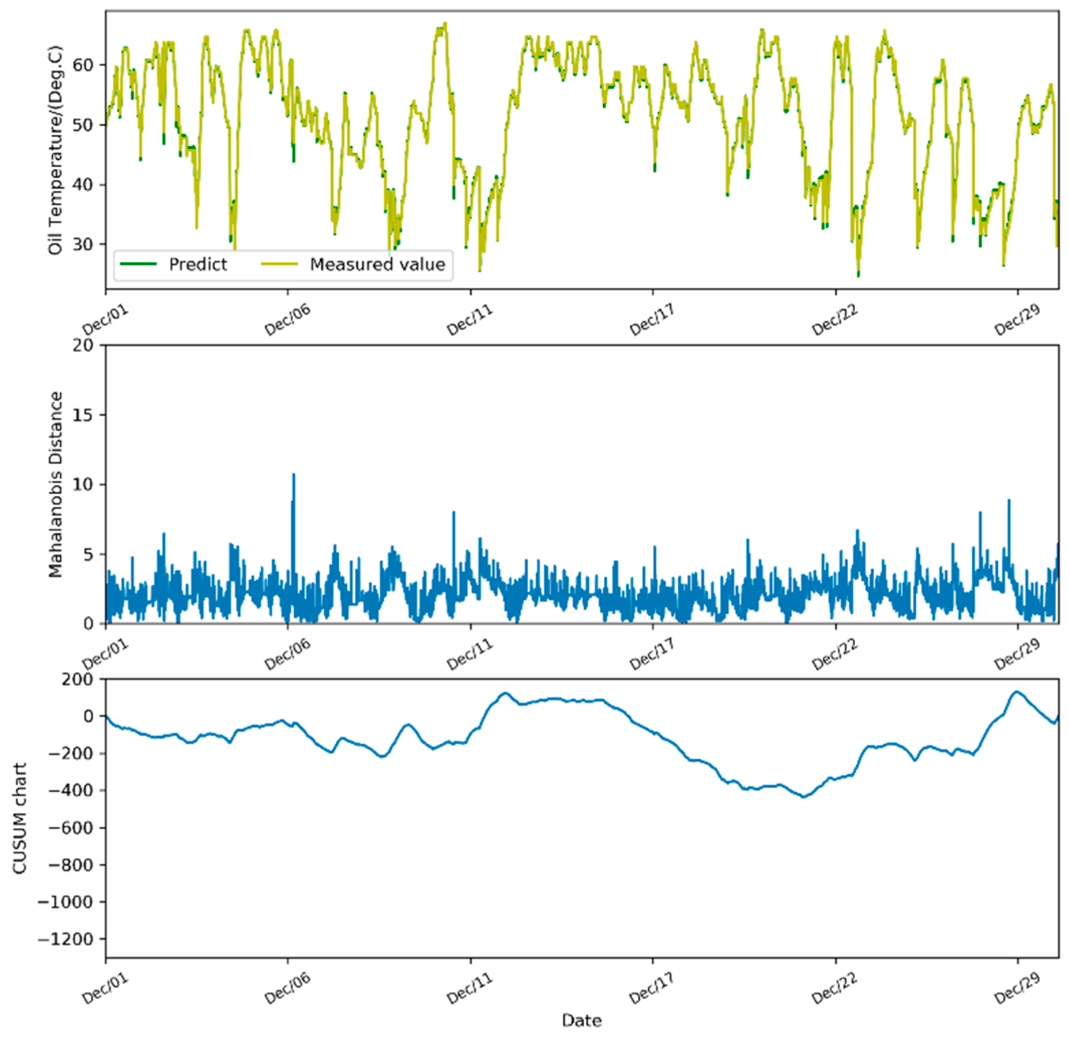
Figure 8 and
Figure 10 as examples. They display the test results on normal turbines and fault turbines respectively. There is an obvious difference between their CUSUM control chart. The CUSUM chart of normal turbines (
Figure 8) may fluctuate slightly in the short term, but the trend in the one-month period is relatively stable, with its absolute value fluctuating from 0 to 500. While for the fault turbines in
Figure 10, the CUSUM chart has a steeper trend and especially when the fault happens, there is a sudden change in direction of CUSUM with their absolute values changing from 0 to 1600. In future work, the appropriate prediction interval should be selected in the application process to reduce the false alarm rate. In addition, the proposed approach will be applied for fault prediction of other components of the wind turbine.


