Abstract
The subcritical polyethylene-reflected plutonium (PERP) metal fundamental physics benchmark, which is included in the Nuclear Energy Agency (NEA) International Criticality Safety Benchmark Evaluation Project (ICSBEP) Handbook, has been selected to serve as a paradigm illustrative reactor physics system for the application of the Second-Order Adjoint Sensitivity Analysis Methodology (2nd-ASAM) that was developed by Cacuci. The 2nd-ASAM enables the exhaustive deterministic computation of the exact values of the 1st-order and 2nd-order sensitivities of a system response to the parameters underlying the respective system. The PERP benchmark is numerically modeled in this work by using the deterministic multigroup neutron transport equation discretized in the spatial and angular independent variables. Thus, the numerical model of the PERP benchmark developed includes the following imprecisely known uncertain parameters: 180 group-averaged total microscopic cross sections, 21,600 group-averaged scattering microscopic cross sections, 120 fission process parameters, 60 fission spectrum parameters, 10 parameters describing the experiment’s nuclear sources, and six isotopic number densities. Thus, the numerical simulation model for the PERP benchmark comprises 21,976 uncertain parameters, which implies that, for any response of interest, there are a total of 21,976 first-order sensitivities and 482,944,576 second-order sensitivities with respect to the model parameters. Computing these sensitivities exactly represents the largest sensitivity analysis endeavor ever carried out in the field of reactor physics. Only 241,483,276 are distinct from each other, and some of these turned out to be zero due to the symmetry of the 2nd-order sensitivities. The numerical results for all of these sensitivities, together with discussions of their major impacts, will be presented in a sequence of publications in the Special Issue of Energies dedicated to “Sensitivity Analysis, Uncertainty Quantification and Predictive Modeling of Nuclear Energy Systems”. This work is the first in this sequence, presenting formulas of general use for neutron transport problems, along with the numerical results that were produced by these formulas for the 180 first-order and 32,400 second-order sensitivities of the PERP leakage response with respect to the neutron transport model’s group-averaged isotopic total cross sections. For comparison, this work also presents formulas of general use and numerical results for the 180 first-order and 32,400 second-order sensitivities of the PERP leakage response with respect to the neutron transport model’s group-averaged isotopic capture cross sections. It has been widely believed hitherto that, for reactor physics systems modeled by the neutron transport or diffusion equations, the second-order sensitivities are all much smaller than the first-order ones. However, contrary to this widely held belief, the numerical results that were obtained in this work prove, for the first time ever, that many of the 2nd-order sensitivities are much larger than the corresponding 1st-order ones, so their effects can become much larger than the corresponding effects stemming from the 1st-order sensitivities. For example, the 2nd-order sensitivities of the PERP leakage response cause the expected value of this response to be significantly larger than the corresponding computed value. The importance of the 2nd-order sensitivities increases as the relative standard deviations for the cross sections increase. For the extreme case of fully correlated cross sections, for example, neglecting the 2nd-order sensitivities would cause an error as large as 2000% in the expected value of the leakage response and up to 6000% in the variance of the leakage response. The significant effects of the mixed 2nd-order sensitivities underscore the need for reliable values for the correlations that might exist among the total cross sections, which are unavailable at this time. The 2nd-order sensitivities with respect to the total cross sections also cause the response distribution to be skewed towards positive values relative to the expected value. Hence, neglecting the 2nd-order sensitivities could potentially cause very large non-conservative errors by under-reporting of the response variance and expected value.
1. Introduction
The modeling and analysis of nuclear energy systems requires the synergetic interdisciplinary coupling of concepts from several scientific and engineering fields, including nuclear and atomic physics, materials sciences, heat and mass transfer, systems control theory, and economics. The modeling of specific physical phenomena in any of these component scientific fields already involves large-scale computations while using very large data sets. For example, modeling the physical processes occurring in the nuclear reactor core, which is the “driver” of nuclear energy systems, requires the numerical solution of the neutron and radiation transport equation, which is an integro-differential equation in seven independent variables that involve a very large number of parameters for representing physical processes involving nuclear cross sections, isotopic number densities, etc. These large-scale computational aspects will be highlighted in this work, which will use the subcritical reactor physics benchmark as a representative illustrative paradigm for second-order sensitivity and uncertainty analysis of large-scale systems.
It is known that the adjoint sensitivity analysis methodology is the most efficient procedure for exactly and exhaustively computing all of the 1st-order sensitivities of a system response (i.e., quantity of interest) to the system’s parameters. Wigner [1] pioneered the use of adjoint operators in conjunction with first-order perturbation theory, to compute exactly and exhaustively the first-order sensitivities for linear systems. The large-scale system that was analyzed by Wigner [1] was the linear neutron transport (and also diffusion) model of a nuclear reactor, in which the model response was the reactor’s multiplication factor and the model parameters were the thousands of neutron cross sections influencing the reactor’s behavior. Using the concepts of functional analysis, Cacuci [2,3,4] subsequently conceived and developed the “adjoint sensitivity analysis methodology” for general nonlinear systems. The field of reactor physics has also provided pioneering works [5,6,7,8,9] for computing selected 2nd-order response sensitivities of the system’s effective multiplication factor and reaction rates (and ratios thereof) while using the adjoint neutron transport and/or diffusion equations. It turned out that the 2nd-order relative sensitivities computed in these early works were considerably smaller than the corresponding 1st-order relative sensitivities. These results, combined with the lack of a general procedure for computing exhaustively all of the 2nd-order sensitivities, gave rise to the opinion that “2nd-order sensitivities are generally insignificant in reactor physics”, which may, in turn, have led to diminishing interest in developing efficient methods for computing 2nd-order sensitivities for nuclear engineering systems. While the interest in computing 2nd-order response sensitivities practically vanished in the nuclear engineering field in the 1990s, interest in this topic became increasingly evident in other fields (e.g., structural mechanics, circuit analysis and optimization, atmospheric and earth sciences), mostly driven by the knowledge that 2nd-order (Hessian) sensitivity information accelerates the convergence of optimization algorithms. It is beyond the scope of this work to provide and exhaustive list of references in this regard, but some of the most influential early works on computing 2nd-order sensitivities are described in [10,11,12]. The common limitations of these early methods for computing 2nd-order response sensitivities are: (i) they were all developed for specific, rather than general, applications, for which they usually estimated, rather than exactly and inclusively computed, all of the 2nd-order response sensitivities; and, (ii) they are computationally expensive, requiring large-scale computations per response for a system comprising model parameters.
A breakthrough was achieved by Cacuci [10,11,12], who developed the “Second-Order Adjoint Sensitivity Analysis Methodology (2nd-ASAM)” for exactly and most efficiently computing all of the second-order functional derivatives of model responses to parameters. For a model response comprising model parameters, the 2nd-ASAM requires at most computations for obtaining all of the 2nd-order sensitivities and all 1st-order sensitivities of a model response with respect to the respective model parameters. Furthermore, the 2nd-ASAM simultaneously intrinsically verifies the computations of the mixed second-order partial sensitivities by computing them twice, while using independently derived adjoint functions. The application of the 2nd-ASAM has been illustrated by means analytically solvable linear [13,14,15] and nonlinear [16] benchmark problems, which highlighted the fundamental importance of the 2nd-order sensitivities for causing asymmetries in the response distribution, and causing the “expected value of the response” to differ from the “computed nominal value of the response”. Cacuci and Favorite highlighted the efficiency and accuracy of the 2nd-ASAM [17], who analyzed a multi-region radiation transport benchmark problem in two-dimensional cylindrical geometry. For this benchmark problem, the 2nd-ASAM only needed 12 adjoint particle transport computations (instead of 877 large-scale forward particle transport computations) to obtain exactly all of the 18 first-order sensitivities and 324 second-order sensitivities of the un-collided gamma ray contributions to the detector’s response with respect to the system’s microscopic cross sections, isotopic number densities, and source emission rates.
In addition to the particle transport and removal phenomena considered in [17], nuclear energy systems also include fission and scattering processes. Such systems can be either critical (when the system can be maintained in steady state without an external source of neutrons) or subcritical (when the system’s time-independent state can only be maintained if an external source injects neutrons into the system). Many critical and several subcritical systems have been evaluated and accepted as fundamental physics benchmarks within the Nuclear Energy Agency (NEA) International Criticality Safety Benchmark Evaluation Project (ICSBEP) Handbook [18]. Prominent among the ICSBEP subcritical experiments are several experiments for which the particle source is a 4.5 kg alpha-phase weapons grade plutonium sphere that was originally constructed at Los Alamos National Laboratory in October 1980 [19]. This source became colloquially known as the “BeRP ball”, “BeRP” being an acronym for “beryllium reflected plutonium” since the earliest experiments conducted with this source were aimed at estimating the reactivity worth of beryllium reflectors. Subsequent experiments used the BeRP ball as the source for experiments in which copper, tungsten, nickel, or polyethylene surrounded the BeRP ball (see Ref. [20,21,22,23] and references therein). The polyethylene-reflected, nickel, and tungsten benchmarks have been accepted in the ICSBEP book as fundamental physics benchmarks. For these subcritical benchmarks, the fundamental quantities (i.e., system responses) of interest are singles counting rate, doubles counting rate, and leakage multiplication. It is noteworthy that the response of interest for subcritical systems is the leakage multiplication instead of the “critical multiplication”, which would be of interest for critical systems.
In their computational evaluation of neutron multiplicity measurements for the polyethylene-reflected BeRP ball, Miller et al. [23] noticed that the computational results significantly disagreed with the corresponding measurements of neutron multiplicity. Miller et al. [23] also performed a limited forward sensitivity analysis (using re-computations with perturbed parameter values) of their computed results with respect to the source-detector distance, dead time, isotopic composition, volume, and density. They concluded [23] that “only a subtle variation in the value of the average number of neutrons produced per fission” for 239Pu was able to improve the simulations of the plutonium sphere for all of the cases”, while also noting that they did not take into account “the energy-dependence of the average number of neutrons produced per fission”. Thus, the conclusion/implication in [23] is that the discrepancy between the computational and experimental results is to be entirely assigned to the uncertainty in the ”average number of neutrons produced per fission”. However, the “polyethylene-reflected BeRP ball” contains many more imprecisely known nuclear data parameters, in addition to those that were incidentally investigated in [23]. Therefore, in order to ascertain whether the conclusion/implication in [23] is warranted or not, it is important to compute all of the 1st-order and 2nd-order sensitivities of responses of the “polyethylene-reflected BeRP ball” to the imprecisely known nuclear data underlying this benchmark.
In preparation for the exhaustive 2nd-order sensitivity analysis of the “polyethylene-reflected BeRP ball”, Cacuci [24,25,26] has specialized the 2nd-ASAM [10,11,12] to the generic neutron transport equation that models multiplying subcritical systems comprising fission, scattering, and external neutron sources. In particular, by considering responses that are functionals of the forward and adjoint fluxes, Cacuci [24,25] has generalized to second-order the methodology presented by Gandini [27], while the work [26] on responses that are ratios of functionals of the forward and adjoint fluxes has been generalized to second-order the methodology presented by Stacey [28,29]. This work (and several subsequent works to follow this one, as will be mentioned in the concluding section of this work) will apply the general theoretical formulas derived in [24,25,26] to the “polyethylene-reflected BeRP ball”. All in all, this application constitutes a pioneering demonstration of the unique capabilities of the 2nd-ASAM to overcome the “curse of dimensionality”, which has thus far impeded the exact computation of all of the 1st-order and 2nd-order response sensitivities for systems characterized by large numbers of imprecisely known parameters.
This work is organized, as follows: Section 2 describes briefly the polyethylene-reflected plutonium metal (“polyethylene-reflected BeRP ball”) benchmark, which shall henceforth be called the PERP benchmark, in order to distinguish this benchmark from the other benchmarks, which also used the plutonium sphere (“BeRP Ball”) as the source of particles, but surrounded by materials other than polyethylene. Section 2 also describes the computational tools that will be used to solve the neutron transport equation that models the PERP benchmark. Section 3 reports the numerical results for the vector (comprising 180 elements) of 1st-order sensitivities of the benchmark’s total leakage response with respect to the benchmark’s group-averaged isotopic total cross sections. Section 4 presents the numerical results for the matrix (comprising 32,400 elements) of 2nd-order sensitivities of the benchmark’s leakage response with respect to the benchmark’s group-averaged isotopic total cross sections. These results will highlight the finding that many of the 2nd-order sensitivities are much larger than the corresponding 1st-order sensitivities. Section 5 presents the numerical results for the 180 first-order and 32,400 second-order sensitivities of the benchmark’s leakage response with respect to the group-averaged isotopic capture cross sections, and compares these results to the corresponding results presented in Section 3 and Section 4 for the total cross sections. Section 6 quantifies the effects of the 2nd-order leakage response sensitivities with respect to the isotopic total cross sections on the leakage responses expected value, variance, and skewness, and compares them to the corresponding effects stemming from the 1st-order sensitivities. It is shown that the effects of the 2nd-order sensitivities are very significant; neglecting them would cause large non-conservative errors by under-estimating the response variance and expected value. The 2nd-order sensitivities shift the leakage response’s expected value significantly away from the computed value of the leakage response, and cause asymmetries in the response distribution. Section 7 presents conclusions that highlight the significance of the novel results that were obtained in this work and sets the stage for the subsequent works in this sequel, which will present the results for the 1st- and 2nd-order sensitivities to the remaining imprecisely known nuclear data parameters that characterize the PERP benchmark.
2. Methodology for Computing the Leakage Response of the Polyethylene-Reflected Plutonium Metal Sphere (PERP) Benchmark
The inner sphere of the PERP benchmark has a radius = 3.794 cm and it contains α-phase plutonium. It is surrounded by a spherical shell reflector made of polyethylene of thickness 3.81 cm; the radius of the outer shell containing polyethylene is = 7.604 cm. Table 1 specifies the constitutive materials of the PERP benchmark.

Table 1.
Dimensions and material composition of the polyethylene-reflected plutonium (PERP) benchmark.
The neutron flux distribution within the PERP benchmark is computed by using the PARTISN [30] multigroup discrete ordinates particle transport code to solve the following multi-group approximation of the neutron transport equation with a spontaneous fission source being provided by the code SOURCES4C [31]:
where denotes the external radius of the PERP benchmark, and where
The PARTISN [30] computations used MENDF71X [32] 618-group cross sections collapsed to energy groups, with group boundaries, , as presented in Table 2. The MENDF71X library uses ENDF/B-VII.1 Nuclear Data [33]. The group boundaries, , are user-defined and they are therefore considered to be perfectly-well known parameters.
Table 2.
Energy group structure, in [MeV], for PERP Benchmark computations.
PARTISN [30] uses the discrete-ordinates approximation to discretize the angular variable in the first and second terms on the right side of Equation (3), and it uses a finite-moments expansion in spherical harmonics to approximate the angular variable in the third and fourth terms on the right side of Equation (3). The specific computations in this work were performed while using a P3 Legendre expansion of the scattering cross section, an angular quadrature of S256, and a fine-mesh spacing of 0.005 cm (comprising 759 meshes for the plutonium sphere of radius of 3.794 cm, and 762 meshes for the polyethylene shell of thickness of 3.81 cm). It is convenient to retain the continuous representation in the angular and radial variables since the spatial and angular discretization parameters will not be considered for sensitivity analysis in this work, as in Equation (1). The various quantities in Equations (1)–(4) have their usual meanings for the standard form of the multigroup neutron transport equation [34], as follows:
- The quantity is the customary “group-flux” for group , and is the unknown state-function obtained by solving Equations (1) and (2).
- The vector denotes the outward unit normal vector at each point on the sphere’s outer boundary, denoted as .
- The spontaneous-fission isotopes in the PERP benchmark are “isotope 1” (239Pu) and “isotope 2” (240Pu). The quantity denotes the total number of spontaneous-fission isotopes; for the PERP benchmark, . The spontaneous fission neutron spectrum of 239Pu and, respectively, 240Pu, is approximated by a Watts fission spectrum while using two evaluated parameters, denoted as and , respectively. The decay constant for actinide nuclide is denoted as , and denotes the fraction of decays that are spontaneous fission (the “spontaneous-fission branching fraction”).
- The quantity denotes the atom density of isotope i in material m; , , where denotes the total number of isotopes, and denotes the total number of materials. The computation of uses the well-known expressionwhere denotes the mass density of material m, ; denotes the weight fraction of isotope i in material m; denotes the atomic weight of isotope , ; denotes the Avogadro’s number. For the PERP benchmark, and , but since the respective isotopes are all distinct (i.e., are not repeated) in the PERP benchmark’s distinct materials, as specified in Table 1, it follows that only the following isotopic number densities exist for this benchmark: .
- The quantity represents the scattering transfer cross section from energy group into energy group and it is computed in terms of the -th order Legendre coefficient (of the Legendre-expanded microscopic scattering cross section from energy group into energy group for isotope ), which are tabulated parameters, in the following finite-order expansion:where denotes the order of the respective finite expansion in Legendre polynomial. The variable will henceforth no longer appear in the arguments of the various cross sections since the cross-sections for every material are treated in the PARTISN [30] calculations as being space-independent within the respective material.
- The total cross section for energy group and material , is computed for the PERP benchmark while using the following expression:where and denote, respectively, the tabulated group microscopic fission and neutron capture cross sections for group . Other nuclear reactions, including (n,2n) and (n,3n) reactions, are not present in this benchmark. The expressions in Equations (6) and (7) indicate that the zeroth order (i.e., ) scattering cross sections must be separately considered from the higher order (i.e., ) scattering cross sections, since the former contribute to the total cross sections, while the latter do not.
- To solve Equation (1), PARTISN [30] computes the quantity using directly the quantities , which are provided in data files for each isotope , and energy group , as followsFor the purposes of sensitivity analysis, the quantity , which quantifies the number of neutrons that were produced per fission by isotope and energy group , can be obtained by using the relation , where the isotopic fission cross sections are available in data files for computing reaction rates.
- The quantity denotes the fission spectrum in energy group , and it is defined in PARTISN [30] as a space-independent quantity, as follows:where denotes the isotopic fission spectrum in group , while denotes the corresponding spectrum weighting function.
- The vector , which appears in the expression of the Boltzmann-operator , represents the “vector of imprecisely known model parameters” having 21,976 components, which are presented in Table 3. The mathematical expression of will be defined in the next section.
Table 3. Summary of imprecisely known parameters for the PERP benchmark.
As has been previously mentioned (see also Ref. [20,21,22,23] and references therein), the fundamental quantities (i.e., system responses) of interest for subcritical benchmarks (such as the PERP benchmark) are singles counting rate, doubles counting rate, the leakage multiplication, and the total leakage. The total leakage is physically more meaningful than the count rates, because it does not depend on the detector configuration. For this reason, many systems are characterized for practical applications by their total leakage rather than by the count rate that a particular detector would see at a particular distance. For this reason, this work considers the total leakage from the PERP benchmark to be the paradigm response of interest for sensitivity analysis; sensitivities analyses of counting rates and other responses can be performed in an analogous manner, by following the general ideas that will be presented in this work (and in the subsequent related works).
Mathematically, the total neutron leakage from the PERP sphere, which is denoted as , will depend on all model parameters (indirectly, through the neutron flux) and it is defined, as follows:
Figure 1 shows the histogram plot of the leakage for each energy group for the PERP benchmark. The total leakage computed while using Equation (10) for the PERP benchmark is neutrons/sec.

Figure 1.
Histogram plot of the leakage for each energy group for the PERP benchmark
3. First-Order Sensitivities of the Total Leakage Response of the Polyethylene-Reflected Plutonium (PERP) Metal Sphere Benchmark with Respect to the Parameters Underlying the Benchmark’s Total Cross Sections
The first- and second-order sensitivities of the leakage response defined in Equation (10) will be computed by particularizing the expressions that were provided by Cacuci [24] to the particular model parameters and response pertaining to the PERP benchmark. Therefore, for convenient referencing, the notation that was introduced by Cacuci [24] will also be used in this work. The various macroscopic cross sections, fission spectra, and sources that appear in Equation (1) will depend on imprecisely known model parameters, as will be discussed below.
In view of Equation (7), the total cross section is characterized by the vector of parameters , which is defined, as follows:
where
In Equations (11)–(13), the dagger denotes “transposition”, denotes the microscopic total cross section for isotope and energy group , denotes the respective isotopic number density, and denotes the total number of isotopic number densities in the model. Thus, the vector comprises a total of imprecisely known components (“model parameters”).
In view of Equation (6), the scattering cross section is characterized by the vector of parameters , which is defined, as follows:
where
In view of Equation (8), the quantity in the fission integral depends on the vector of parameters , which is defined, as follows:
with
where denotes the microscopic fission cross section for isotope and energy group , denotes the average number of neutrons per fission for isotope and energy group , and denotes the total number of fissionable isotopes.
The fission spectrum is considered to depend on the vector of parameters , being defined as follows:
In view of Equation (9), the quantities further depend on the parameters , , , , but these latter dependences can be taken into account by applying the chain rule on the 1st-order sensitivities , once these sensitivities have been obtained.
In view of Equation (4), the source depends on the vector of model parameters , which is defined, as follows:
In view of Equations (11)–(20), the model parameters characterizing the PERP benchmark can all be considered to be the components of the following “vector of model parameters:”
Thus, the total number of imprecisely known model parameters for the PERP benchmark is: . Table 3 summarizes these parameters, together with their symbols. Furthermore, the 1st- and 2nd-order sensitivities of the PERP benchmark’s total leakage response to the multigroup microscopic capture cross sections will also be computed and presented in Section 5, for comparing these results to those that were obtained in Section 4 for the sensitivities of the leakage response to the multigroup microscopic total cross sections. Therefore, the last row of Table 3 lists the symbols and number of multigroup microscopic capture cross sections.
The components of the vector of 1st-order sensitivities of the leakage response with respect to the model parameters is denoted as , and it is defined, as follows:
The symmetric matrix of 2nd-order sensitivities of the leakage response with respect to the model parameters is denoted as , and it is defined, as follows:
The expressions and numerical values of the components of and have been obtained by particularizing the general results presented by Cacuci [24]. Evidently, the complete results cannot be reported in a single article. Therefore, this work will only report the results for the 1st- and 2nd-order sensitivities of the leakage response with respect to the group-averaged total microscopic cross sections, namely the vector and the matrix . The 1st-order sensitivities of the leakage response to the model parameters that underlie the total cross section are computed from the following particular form of Equation (150) in [24]:
where the multigroup adjoint fluxes are the solutions of the following particular form of 1st-Level Adjoint Sensitivity System (1st-LASS) that is presented in Equations (156) and (157) of [24]:
where is the radius of the PERP sphere, and where
As detailed in [30], the PARTISN solver module solves the adjoint transport equation by transposing (in energy) the matrices of scattering cross sections and inverting the group order of the problem. The transposition of the scattering matrix converts a downscattering problem to an upscattering problem, so that, the problem will execute in a downscatter-like mode by inverting the group order. In addition to transposing the scattering matrices, the fission source term in the transport equation is also transposed, so that the summation becomes , where and where the quantity denotes the weights in angle while the quantity denotes the total number of angular discretization. The code does not transpose the angular direction matrix that is associated with the leakage terms in the transport equation. Instead, the adjoint calculation of the leakage operator proceeds as in the direct (forward) calculation, but the results of the adjoint calculation for direction must be identified as the adjoint solution for direction . For example, the vacuum boundary condition at a surface (no incoming angular flux) in an adjoint calculation must be interpreted as a condition of no outgoing flux. Likewise, the adjoint leakage at a surface is “incoming” instead of “outgoing”.
For the PERP benchmark, the following relations hold:
where the subscripts , , and denote the isotope, the energy group, and material associated with the parameter , respectively; and, denote the Kronecker-delta functionals (e.g., if ; if ). Inserting Equation (28) into Equation (24) yields the following expression for computational purposes:
The numerical values of the 1st-order relative sensitivities for the six isotopes contained in the PERP benchmark will be presented in Section 4, below, in tables that will also include comparisons with the numerical values of the corresponding 2nd-order relative sensitivities .
4. Second-Order Sensitivities of the PERP Total Leakage Response with Respect to the Parameters Underlying the Benchmark’s Total Cross Sections
The expressions of the 2nd-order sensitivities of the leakage response to the parameters that underlie the total cross section will be obtained in this Section by starting with the following general result presented in Equation (158) by Cacuci [24]:
where the 2nd-level adjoint functions and , are the solutions of the following 2nd-Level Adjoint Sensitivity System (2nd-LASS) that is presented in Equations (164)–(166) of [24]:
For the PERP benchmark, when the parameters and correspond to the total cross sections, i.e., and , respectively, the following relations hold:
where the subscripts , and denote the isotope, the energy group and material associated with the parameter , respectively. Inserting Equations (35)–(37) into Equations (30), (31) and (33) yields the following expression for the 2nd-order sensitivities of the leakage response to the parameters involved in the definitions of the total cross sections:
where the 2nd-level adjoint functions and , are the solutions of the following particular forms of Equations (31) and (33):
subject to the boundary conditions shown in Equations (32) and (34). All of the quantities appearing in Equations (38)–(40) are evaluated at the nominal values of all the model parameters.
The 2nd-order absolute sensitivities of the leakage response with respect to the total cross sections, i.e., , for the isotopes and energy groups of the PERP benchmark are computed while using Equation (38). The (Hessian) matrix of 2nd-order absolute sensitivities has dimensions , since . The matrix of 2nd-order relative sensitivities, denoted as , is defined, as follows:
The numerical results obtained for the matrix have been partitioned into submatrices, each of dimensions , and the summary of the main features of each submatrix is presented in Table 4. The matrix is symmetric, so only the results for the upper triangular submatrices are presented in the following form: when a submatrix comprises elements with relative sensitivities with absolute values that are greater than 1.0, the total number of such elements are counted and shown in the shaded cells of the table. Otherwise, if the relative sensitivities of all the elements of a submatrix have values that lie in the interval , only the element having the largest absolute value in the submatrix is listed in Table 4, together with the phase-space coordinates of that element. The sub-matrices in Table 4, which comprise components with absolute values greater than 1.0, will be discussed in detail in subsequent sub-sections of this Section.
Table 4.
Summary presentation of the matrix .
4.1. Second-Order Unmixed Relative Sensitivities
The 2nd-order unmixed sensitivities , are particularly important, since, as will be shown in Section 6, below, these sensitivities will contribute to the moments (namely: expected values, variances/covariances, skewness) of the response distribution, even when the model parameters are uncorrelated. The term “unmixed” denotes the 2nd-order sensitivity with respect to the same parameter, and the term “mixed” denotes the 2nd-order sensitivity with respect to different parameters. Furthermore, the values of these unmixed 2nd-order relative sensitivities of the response to the model parameters can be directly compared to the values of the 1st-order relative sensitivities . These comparisons are presented in Table 5, Table 6, Table 7, Table 8, Table 9 and Table 10 for the six isotopes that are contained in the PERP benchmark. Thus, Table 5 presents a side-by-side comparison of 1st-order relative sensitivities and 2nd-order relative sensitivities for isotope 1 (239Pu) and for all energy groups . This comparison indicates that the values of the 2nd-order sensitivities are generally greater than the corresponding values of the 1st-order sensitivities for the same energy group. The largest values (shown in bold in the table) for both the 1st-order and 2nd-order relative sensitivities are for the 12th energy group, while the next largest values are for the 13th energy group. It is noteworthy that all of the 1st-order relative sensitivities are negative, which signifies that an increase in will cause a decrease in .
Table 5.
Comparison of 1st-order relative sensitivities and 2nd-order relative sensitivities for isotope 1 (239Pu).
Table 6.
Comparison of 1st-order relative sensitivities and 2nd-order relative sensitivities for isotope 2 (240Pu).
Table 7.
Comparison of 1st-order relative sensitivities and 2nd-order relative sensitivities for isotope 3 (69Ga).
Table 8.
Comparison of 1st-order relative sensitivities and 2nd-order relative sensitivities for isotope 4 (71Ga).
Table 9.
Comparison of 1st-order relative sensitivities and 2nd-order relative sensitivities for isotope 5 (C).
Table 10.
Comparison of 1st-order relative sensitivities and 2nd-order relative sensitivities for isotope 6 (1H).
The results that are presented in Table 6, Table 7, Table 8 and Table 9 indicate that both the 1st-order and 2nd-order unmixed sensitivities for the isotopes 240Pu, 69Ga, 71Ga, and C, respectively, are very small. Furthermore, the 1st-order relative sensitivities are all greater than the 2nd-order relative sensitivities, except for the 2nd-order unmixed sensitivities of the leakage with respect to the total cross section of Carbon in the lowest-energy group. For the isotopes 240Pu, 69Ga, 71Ga, the largest values for both the 1st-order and 2nd-order relative sensitivities are for the 12th energy group. For the isotope C, the largest values for both the 1st-order and 2nd-order relative sensitivities are for the 30th, i.e., the lowest energy group. It is noteworthy that all of the 1st-order relative sensitivities that are presented in Table 6, Table 7, Table 8 and Table 9 are negative, which signify that an increase in the corresponding microscopic cross sections will cause a decrease in the value of the response (i.e., fewer neutrons will leak out of the sphere).
As shown in Table 6, Table 7, Table 8 and Table 9, the 1st-order relative sensitivities are all greater than the 2nd-order relative sensitivities for isotopes 2, 3, 4, and 5 (with one exception, for isotope 5 at g = 30). However, the results that are presented in Table 5 and Table 10 indicate that, for isotope 1 (239Pu) and isotope 6 (1H), the 1st-order relative sensitivities are generally smaller than the 2nd-order relative sensitivities. For isotope 6 (1H), the largest relative sensitivities (marked in bold digits) occur for the lowest-energy group. Remarkably, the respective 2nd-order unmixed sensitivity is larger by a factor of about 50 than the corresponding 1st-order relative sensitivity. As for the other isotopes comprising the PERP sphere, all of the 1st-order relative sensitivities that are presented in Table 9 are negative, which signify that an increase in the corresponding microscopic group cross sections of 1H will also cause a decrease in the value of the response (i.e., fewer neutrons will leak out of the sphere). All in all, the results in Table 5, Table 6, Table 7, Table 8, Table 9 and Table 10 indicate that largest 1st- and 2nd-order sensitivities, and hence the most important consequent effects, arise from the total microscopic cross sections of isotopes 1H and 239Pu.
All the values for the 1st-order and unmixed 2nd-order relative sensitivities, as shown in Table 5, Table 6, Table 7, Table 8, Table 9 and Table 10, have been independently verified with the results being obtained from the central-difference estimates by repeated forward PARTISN computations, in which the isotopic cross section for each group was perturbed by a small amount at a time. These verifications showed good agreement between the sensitivities that were computed while using the 2nd-LASS and the corresponding ones that were computed using central-difference methods. For the large sensitivities in group 30, the verifications were as follows:
- (1)
- As shown in Table 10, the 2nd-LASS-computed 1st-order relative sensitivity for the 30th group of isotope 1H has the value −9.366; the value of the corresponding absolute sensitivity computed using the central-difference method is −5.59657 × 10⁵, which yields the relative sensitivity value ; the two values agree well with one another.
- (2)
- As shown in Table 10, the 2nd-LASS-computed unmixed 2nd-order relative sensitivity for the 30th group of isotope 1H has the value of 429.6; the value of the corresponding absolute sensitivity computed while using the central-difference method is 8.706316 × 10⁵, which yields the relative sensitivity value ; the two values agree well with one another.
- (3)
- As shown in Table 9, the 2nd-LASS-computed unmixed 2nd-order relative sensitivity for the 30th group of isotope C has the value of 3.016; the value of the corresponding absolute sensitivity computed while using the central-difference method is 2.179357 × 10⁵, which yields the relative sensitivity value ; the two values show good agreement with each other.
Additional verifications of the results shown in Table 4, Table 5, Table 6, Table 7, Table 8, Table 9 and Table 10, especially for the large sensitives for group 30 of isotopes C and 1H, the neutron flux was re-computed by using PARTISN [30] that was coupled to the spontaneous fission source computed while using the code MISC [35] instead of SOURCES4C [31]. MISC provides an alternative to SOURCES4C for computing the source for the neutron transport equation. The sensitivities of the leakage response to the total cross sections obtained by using PARTISN+MISC agree very well with those obtained while using PARTISN+SOURCES4C. For example, MISC+PARTISN yields the values −9.36595 and 429.627, respectively, for the 1st- and 2nd-order relative sensitivities to the 30th group of the total cross section for isotope 1H. These values match very well the corresponding values of −9.36599 and 429.643, respectively, which were obtained using PARTISN+SOURCES4C, as listed in Table 10. These additional independent verifications (using PARTISN+MISC) of the results obtained using the coupled codes PARTISN+SOURCES4C alleviate any concerns regarding the accuracy of the computations of the spontaneous fission source for the PERP benchmark.
4.2. Second-Order Mixed Relative Sensitivities for the Leakge Response with respect to the Microscopic Total Cross Sections of Isotope 239Pu,
Figure 2 depicts the results that were obtained for , , referring to 239Pu. This matrix is symmetrical, of course, with respect to its principal diagonal. As shown in this figure, 98 elements have relative sensitivities greater than 1.0, the majority (93 out of 98) of which are concentrated in the energy region that was confined by the energy groups and . Table 11 presents the actual numerical values of these elements. The largest value among these sensitivities is attained by the relative 2nd-order unmixed sensitivity of the leakage response with respect to the total cross section, , of 239Pu in energy group 12.
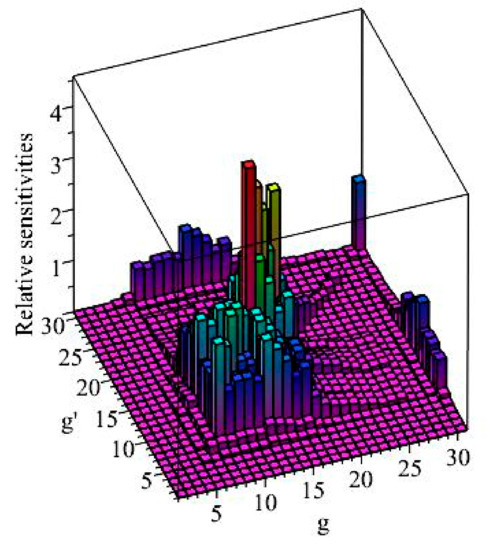
Figure 2.
The matrix of sensitivities for 239Pu.
Table 11.
Components of having values greater than 1.0.
In addition to the sensitivities presented in Table 11, the following 2nd-order relative sensitivities of the leakage response with respect to the group-averaged total microscopic cross sections of 239Pu are greater than 1.0: , , and .
4.3. Second-Order Mixed Relative Sensitivities for the Leakge Response with Respect to the Microscopic Total Cross Sections of Isotope 239Pu and Isotope C,
The -matrix, , comprising the 2nd-order relative sensitivities of the leakage response with respect to the total microscopic cross sections of isotope 1 (239Pu) and isotope 5 (C), has just 10 components that have absolute values greater than 1.0; Table 12 presents these components. All of these components involve the total cross section , which corresponds to the lowest energy group of isotope 5 (C).
Table 12.
Components of having values greater than 1.0.
4.4. Second-Order Mixed Relative Sensitivities for the Leakge Response with Respect to the Microscopic Total Cross Sections of Isotope 239Pu and Isotope 1H,
Figure 3 depicts the mixed relative sensitivities of the leakage response with respect to the total cross sections of isotope 1 (239Pu) and isotope 6 (1H). This figure comprises 135 mixed 2nd-order relative sensitivities having values that are greater than 1.0, the large majority of which are concentrated in the energy region confined by the energy groups and , respectively. The largest of these sensitivities is ; the second largest value is . Table 13 and Table 14 present the 135 elements of the sensitivity matrix, , which have relative sensitivity values that are greater than 1.0.

Figure 3.
The matrix of sensitivities , for 239Pu and 1H.
Table 13.
Components of having values greater than 1.0.
Table 14.
Continuation of Table 13.
4.5. Second-Order Mixed Relative Sensitivities for the Leakge Response with Respect to the Microscopic Total Cross Sections of Isotope 240Pu and Isotope 1H,
Only three components of the sensitivity matrix , of the 2nd-order sensitivities of the leakage response with respect to the total cross sections of isotope 2 (240Pu) and isotope 6 (1H) have values greater than 1.0. These three sensitivities are: , , and , all involving the total cross section of isotope 6 (1H).
4.6. Second-Order Mixed Relative Sensitivities for the Leakge Response with Respect to the Microscopic Total Cross Sections of Isotope C,
A single component of the sensitivity matrix , of 2nd-order sensitivities of the leakage response with respect to the total cross sections of isotope 5 (C) is larger than 1.0, namely .
4.7. Second-Order Mixed Relative Sensitivities for the Leakge Response with Respect to the Microscopic Total Cross Sections of Isotope C and Isotope 1H,
As presented in Table 15, there are 33 elements in the sensitivity matrix , of 2nd-order sensitivities of the leakage response with respect to the total cross sections of isotope 5 (C) and isotope 6 (1H), which have values that are greater than 1.0. Specifically, 18 out of the 33 elements involve the cross section for group of isotope 6 (1H), and the other 15 elements involve the cross section for group of isotope 5 (C).
Table 15.
Components of having values greater than 1.0.
4.8. Second-Order Mixed Relative Sensitivities for the Leakge Response with Respect to the Microscopic Total Cross Sections of Isotope 1H,
Figure 4 depicts the matrix , comprising the 2nd-order relative sensitivities of the leakage response with respect to the total cross sections of isotope 6 (1H). This submatrix is symmetrical regarding its principal diagonal.
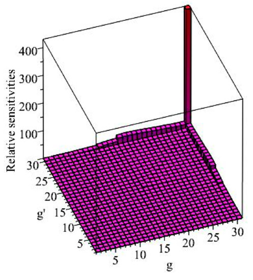
Figure 4.
The matrix of sensitivities , for 1H.
Of the 900 components of that are depicted in Figure 4, 259 components have relative sensitivities greater than 1.0, which are also listed in Table 16 and Table 17. The unmixed 2nd-order sensitivity , of the leakage response with respect to , is the largest of all 2nd-order sensitivities. The 2nd-order sensitivity of the leakage response with respect to the parameters and , namely, , is the second largest. Thirty-six (36) additional sensitivities that involve energy groups and energy groups have values larger than 5.0. In addition to the sensitivities presented in Table 16 and Table 17, the following sensitivities are also larger than 1.0: , , , and .
Table 16.
Components of , having values greater than 1.0.
Table 17.
Continuation of Table 16.
5. First- and Second-Order Sensitivities of the PERP Total Leakage Response with Respect to the Parameters Underlying the Benchmark’s Capture Cross Sections
As indicated in Equation (7), the capture cross section is one of the components of the total cross section. The total cross section reduces to the capture cross section in a purely absorbing medium. Therefore, it is of interest to compute the 1st- and 2nd-order sensitivities of the PERP benchmark’s leakage response with respect to the capture cross sections and compare these results with the results that were obtained in Section 4 for the sensitivities with respect to the corresponding total cross sections. Analogous to the definition given in Equation (13), it is convenient to define the vector of parameters corresponding to the microscopic capture cross section, which is defined, as follows:
5.1. First-Order Sensitivities
The 1st-order sensitivities of the leakage response to the capture cross sections are computed while using the following particular form of Equation (150) in [24]:
The following relations hold:
Inserting Equation (44) into Equation (43) yields the following expression for computational purposes:
The right hand side of Equation (45) is the same as that in Equation (29), which indicates that the first-order absolute sensitivities of the leakage response with respect to the microscopic capture cross sections are identical to those with respect to the corresponding microscopic total cross sections, namely, . However, the relative sensitivities of the leakage response with respect to the microscopic total cross sections will differ from the relative sensitivities of the leakage response with respect to the microscopic capture cross sections.
The numerical values of the 1st-order relative sensitivities of the leakage to the capture cross sections, , will be presented in Section 5.3, in tables together with the numerical values of the corresponding unmixed 2nd-order relative sensitivities , for all six isotopes contained in the PERP benchmark.
5.2. Second-Order Sensitivities
The equation that is needed for deriving the expression of the 2nd-order sensitivities is obtained by particularizing Equation (158) in [24] to the PERP benchmark, in conjunction with the relations , , and , which leads to the following expression:
where the 2nd-level adjoint functions and , are the solutions of the following 2nd-Level Adjoint Sensitivity System that is presented in Equations (164)–(166) of [24]:
In Equations (47) and (49), the parameter corresponds to the capture cross section indexed by , i.e., . Inserting Equation (44) into Equations (47) and (49), yields the following particular expressions:
It is noteworthy that Equations (51) and (52) are the same as Equations (39) and (40), respectively. Thus, the 2nd-Level Adjoint Sensitivity System for the capture cross sections (comprising Equations (48), and (50)–(52)) is formally identical to the 2nd-LASS for the total cross sections [comprising Equations (32), (34), (39) an(40)]. Consequently, the 2nd-level adjoint functions , and for the capture cross sections are formally identical to the 2nd-level adjoint functions for the total cross sections.
In Equation (46), the parameters and correspond to the capture cross sections, i.e., and , respectively; therefore, the following relations hold:
Inserting Equations (53) and (54) into Equation (46) yields the following expression for the 2nd-order sensitivities of the leakage response with respect to the microscopic capture cross sections:
The right hand side of Equation (55) is formally identical to the right side of Equation (38), which indicates that the absolute 2nd-order sensitivities of the leakage response with respect to the microscopic capture cross sections are exactly the same as that with respect to the corresponding microscopic total cross sections, namely, .
5.3. Numerical Results for
The 2nd-order absolute sensitivities of the leakage response with respect to the capture cross sections, i.e., , for the isotopes and energy groups of the PERP benchmark are computed while using Equation (55). The matrix has dimensions , since . The relative sensitivities that correspond to , are denoted as and they are defined, as follows:
Comparing Equation (56) to Equation (41) reveals that the respective expressions are not identical. Thus, although the absolute 2nd-order sensitivities of the leakage response with respect to the microscopic capture cross sections are exactly the same as that with respect to the corresponding microscopic total cross sections, the respective relative sensitivities are scaled by the factor .
Table 18 presents the summary of the numerical results that were obtained for the elements of the matrix , partitioned into submatrices, each having dimensions . Table 18 only presents the results for the upper triangular submatrices since the matrix is symmetrical. As shown in Table 18, the values of the mixed 2nd-order relative sensitivities in the matrix are all smaller than 1.0, and they are mostly positive. Among all of the elements in the matrix, a total of 3464 out of 3600 elements have positive values. The remaining 136 elements of this matrix have negative values, which are all related to the capture cross sections of isotopes C and 1H, and their values are very close to zero (e.g., in the order of ). The overall maximum relative sensitivity in the matrix is . The results in Table 18 also indicate that the largest sensitivities in each of the respective submatrices mostly involve the capture cross sections for the 30th energy group, and they otherwise involve the capture cross sections for the 22th, 23th, and 27th energy groups of the isotopes.
Table 18.
Summary presentation of the matrix .
The 2nd-order unmixed sensitivities of the leakage response with respect to the capture cross sections, which are the elements on the diagonal of the matrix , can be directly compared to the values of the 1st-order relative sensitivities . Likewise, all of the values for the 1st-order and unmixed 2nd-order relative sensitivities to the capture cross sections, as shown in Table 19, Table 20, Table 21, Table 22, Table 23 and Table 24, have been independently verified while using re-computations with suitably altered parameter values in conjunction with central-difference formulas. The side-by-side comparisons that are shown in Table 19, Table 20, Table 21, Table 22, Table 23 and Table 24 for all six isotopes of the PERP benchmark indicate that, for each isotope, the values of both the 1st-order and the unmixed 2nd-order relative sensitivities are very small, and the unmixed 2nd-order sensitivity are generally smaller than the corresponding values of the 1st-order sensitivity for the same energy group. As also shown in these tables, all of the 1st-order relative sensitivities are negative, which signifies that an increase in will cause a decrease in the total leakage, ; and, all of the unmixed 2nd-order sensitivities are positive.
Table 19.
Comparison of 1st-order relative sensitivities and 2nd-order unmixed relative sensitivities to the capture cross sections for isotope 1 (239Pu).
Table 20.
Comparison of 1st-order relative sensitivities and 2nd-order relative sensitivities to the capture cross sections for isotope 2 (240Pu).
Table 21.
Comparison of 1st-order relative sensitivities
and 2nd-order relative sensitivities to the capture cross sections for isotope 3 (69Ga).
Table 22.
Comparison of 1st-order relative sensitivities and 2nd-order relative sensitivities to the capture cross sections for isotope 4 (71Ga).
Table 23.
Comparison of 1st-order relative sensitivities and 2nd-order relative sensitivities to the capture cross sections for isotope 5 (C).
Table 24.
Comparison of 1st-order relative sensitivities and 2nd-order relative sensitivities to the capture cross sections for isotope 6 (1H).
It is revealing to make the following comparisons:
- (i)
- (ii)
- (iii)
- (iv)
- (v)
- (vi)
The above comparisons indicate that, for each isotope, the values for both the 1st-order and unmixed 2nd-order relative sensitivities of the leakage response with respect to the capture cross sections are much smaller than those of the corresponding total cross sections for the same energy group. This is because the values for the 1st-order sensitivities and, respectively, unmixed 2nd-order relative sensitivities with respect to the capture cross sections are scaled down from the corresponding relative sensitivities to the total cross sections by factors of and , respectively.
6. Second-Order Uncertainty Analysis of the PERP Leakage Response
Knowledge of the first- and second-order sensitivities is required to compute the following moments of the response distribution:
- (i)
- Up to 2nd-order response sensitivities, the 1st-order moment (expected values) of a response has the following expression [12]:where denotes the correlation coefficient between parameters and , while denotes the standard deviation of the model parameter .
- (ii)
- Up to 2nd-order response sensitivities, the 2nd-order moment (covariance) of two responses has the following expression [12]:where and denote the triple-correlations and, respectively, the quadruple correlations among the respective parameters.
- (iii)
- Up to 2nd-order response sensitivities, the 3rd-order moment of three responses has the following expression [12]:
In particular, the skewness of a single response, , which indicates the degree of the distribution’s asymmetry with respect to its mean, is defined, as follows:
6.1. Uncorrelated Total Microscopic Cross Sections
Correlations among the group total cross sections are not available for the PERP benchmark under consideration. When such correlations are unavailable, the maximum entropy principle (see, e.g., [36]) indicates that neglecting them by setting in Equations (57)–(59) minimizes the inadvertent introduction of spurious information into the computations of the various response moments. Thus, only considering the contributions from the group-averaged uncorrelated total microscopic cross sections, the expected value of the leakage response has the following expressions:
where the superscript “(2,U)” indicates “2nd-order, uncorrelated” cross sections, the subscript “t” indicates contributions solely from the group-averaged total microscopic cross sections, and where the quantity denotes second-order contributions to the expected value, of the leakage response , and it is given by the following expression:
In Equation (62), the quantity denotes the standard deviation that is associated with the model parameter .
Third- and fourth-order correlations for the group-averaged microscopic total cross sections are not available in the open literature, so their effects on the uncertainties that they would cause in the leakage response cannot be exactly quantified at this time. In the absence of any information whatsoever regarding the triple correlations among the total group-averaged microscopic cross sections, the most “reasonable” assumption (in the sense of introducing the least amount of spurious information into the system, according to the maximum entropy principle [36]) is to set them to zero in Equations (58) and (59). Actually, setting is rigorously correct if the total group-averaged microscopic cross section were considered to be multivariate correlated normally distributed quantities. In such a case, it is also well known that the following relation holds for the quadruple correlations :
Taking into account contributions solely from the group-averaged uncorrelated and normally-distributed total microscopic cross sections (which will be indicated by using the superscript “(U,N)” in the following equations), the expression for computing the variance, denoted as , of the leakage response of the PERP benchmark takes on the following particular form of Equation (58):
where the first-order contribution term, , to the variance is defined as
while the second-order contribution term, , to the variance is defined, as follows:
Again taking into account contributions solely from the group-averaged uncorrelated normally-distributed total microscopic cross sections, the third-order moment, , of the leakage response for the PERP benchmark takes on the following particular form of Equation (59):
As Equation (67) indicates, if the 2nd-order sensitivities were unavailable, the third moment —and hence the skewness of the leakage response—would vanish and the response distribution would by default be assumed to be Gaussian.
The skewness, , of the leakage response, , due to the variances of uncorrelated and normally distributed microscopic total cross sections is defined, as follows:
6.2. Fully Correlated Total Microscopic Cross Sections
The effects of correlations among the group-averaged microscopic total cross sections, and hence the impact of the second-order mixed sensitivities of the leakage response to these cross sections, can be quantified in the extreme case of fully correlated cross sections. When the cross sections are fully correlated, all of the correlation coefficients in Equations (57)–(59) are unity.
Thus, if the group-averaged microscopic total cross sections were fully correlated (denoted using the superscript “FC”, the expression of the expected value, , of the leakage response would not be as given in Equation (61), but would instead be given by the following expression:
where the quantity denotes the contributions from both the unmixed and mixed 2nd-order sensitivities when the total cross sections parameters are fully correlated, which is given by the following expression:
The additional 2nd-order contributions to the expectation value of the leakage response when the total cross sections are fully correlated is denoted as , where the superscript “MSC” denotes “mixed second-order correlated”, and it is computed while using the following expression:
For fully correlated () and normally-distributed total cross sections, the use of Equation (63) together with Equations (64)–(67) reduces Equation (58) to the following expression:
In Equation (72), denotes the variance that would be induced in the leakage response if the total microscopic cross sections were fully correlated and normally-distributed [indicated by the superscript “(FC,N)”], denotes the contributions from the 1st-order sensitivities when the total cross sections parameters are fully correlated, and it is given by the following expression:
and denotes the contributions from both the mixed and unmixed 2nd-order sensitivities when the total cross sections parameters are fully correlated and normally distributed, and it is given by the following expression:
The contributions to involving the first-order sensitivities will be denoted as , where the superscript “(1, MSC)” denotes “first-order, mixed sensitivities, correlated”, and they are obtained by subtracting the uncorrelated terms from the fully correlated ones, i.e.,
The contributions to involving the second-order sensitivities will be denoted as and they are obtained by subtracting the respective uncorrelated terms from the respective fully correlated ones, i.e.,
For fully correlated total cross sections, the use of Equation (63) together with Equations (64)–(67) reduces Equation (59) to the following expression, in which the 3rd-order sensitivities have been neglected:
The contributions stemming from the mixed 2nd-order sensitivities when the total cross sections are fully correlated and normally distributed will be denoted as , where the superscript “(MSC,N)” indicates “Mixed Second-order sensitivities, fully Correlated Normally distributed parameters”. These contributions are computed by subtracting the uncorrelated terms, , from the respective fully correlated ones, , to obtain:
For fully correlated total cross sections, the skewness, , is defined as usual:
6.3. Numerical Results
The effects of the first- and second-order sensitivities on the response moments (expected value, variance, and skewness) can be quantified by considering uniform values for the standard deviations of the group-averaged isotopic total microscopic cross sections and using these values together with the respective sensitivities computed in Section 4 in Equations (61)–(79). The typical values for group-averaged microscopic total cross sections range from about 1% to about 15%. Thus, a 1% relative standard deviation can be considered to be “very small”, a 5% relative standard deviation can be considered to be “typical”, and a 10% relative standard deviation can be considered to be “large”. Table 25 and Table 26 present the results thus obtained.
Table 25.
Response moments for various relative standard deviations of total microscopic cross sections that are uncorrelated.
Table 26.
Response moments for various relative standard deviations of total microscopic cross section which are fully correlated.
6.3.1. Very Small (1%) Relative Standard Deviations
When the total cross sections are considered to be uncorrelated and the respective standard deviations are assumed to be very small (1%), the effects of the 2nd-order sensitivities, through to the expected response value are negligibly small, so that the expected value differs very little from the response’s nominal value, , computed while using the nominal parameter values. The fact the and, consequently, indicates that the mixed 2nd-order sensitivities are at least as important as the unmixed 2nd-order sensitivities, but even in the fully-correlated case, the 2nd-order sensitivities do not appreciably affect the expected response value for 1% relative standard deviations in the total microscopic cross sections. This result is not surprising, since the response is expected to behave almost linearly for very small (1%) parameter variations, so the nonlinear effects, quantified by the 2nd-order sensitivities, are expected to be insignificant.
For uncorrelated total cross sections, and , indicate that the contributions of the 2nd-order sensitivities to the response variance are smaller than the contributions stemming from the 1st-order sensitivities. However, , which indicates that the mixed 2nd-order sensitivities are significantly more important than the unmixed 2nd-order sensitivities in contributing to the response’s variance. Finally, , which indicates that the 2nd-order sensitivities give rise to a positive response skewness, thus causing the response distribution to be asymmetrically “skewed” towards the “right”, in the “positive direction”, of the response’s expected value .
The relation indicates that the cross section correlations and mixed 2nd-order sensitivities are important because they skew the response distribution even more towards the “positive direction” than in the absence of correlations.
6.3.2. Typical (5%) Relative Standard Deviations
The second column from the right in Table 25 and Table 26 present the results that were obtained by assuming that the relative standard deviations of the group-averaged microscopic total cross sections were all 5%. Comparing the results shown in this column to the results discussed above for standard deviations of 1% indicates that all of the trends observed for the “1% case” are magnified in the “5% case”. Thus, for uncorrelated cross section, , indicating that the 2nd-order contribution have become comparable to the computed leakage value , thus causing a significant shift, by about 40%, of the expected value for the leakage response by comparison to the computed value . This shift is even more pronounced when the cross sections are fully correlated, in which case , which indicates that the effects of the mixed 2nd-order sensitivities are much larger than the effects of the unmixed 2nd-order sensitivities. Thus, the customary procedure of neglecting second (and higher) order sensitivities and considering that the computed value, , is the actual expected (i.e., mean) value of the distribution, would be about 40% in error if the cross sections were uncorrelated and even more severely in error (by ca 700%) if the cross sections were fully correlated, for typical (5%) relative standard deviations in the total cross sections.
For uncorrelated cross sections, the second-order unmixed sensitivities contribute over 68%, through the quantity , to the response variance . On the other hand, if the cross sections were fully correlated, the effects of the mixed 2nd-order sensitivities would greatly accentuate this trend, as evidenced by the relations and . The skewness remains positive, but the relation indicates that the effects of the mixed 2nd-order sensitivities are to reduce the skewness and thus render the distribution of the total cross sections more symmetric regarding its expected value.
6.3.3. Large (10%) Relative Standard Deviations
The trends that were displayed by the results for a uniform standard deviation of 5% for the group isotopic microscopic cross sections are significantly amplified when this uniform standard deviation is increased to 10%. Thus, the 2nd-order contribution for uncorrelated cross sections is 260% larger than the computed leakage value , contributing 72% of the expected value for the leakage response by comparison to 28% contributed by the computed value . For fully correlated cross sections, the results that are presented in Table 26 indicate that , highlighting the very significant impact of the mixed 2nd-order sensitivities on causing the expected value of the leakage response to significantly differ from the computed response value, since, as shown by the results that are presented in Table 26, . Thus, the customary procedure of neglecting second (and higher) order sensitivities and considering that the computed value, , as the actual expected (i.e., mean) value of the distribution, would be in error by anywhere from 360% to 2000%.
Furthermore, for uncorrelated cross sections, the contribution of the unmixed 2nd-order sensitivities to the response variance is 847% larger than the contribution stemming from the first-order sensitivities. Hence, neglecting these 2nd-order contributions would cause a very large non-conservative error by under-reporting the response variance by a factor of 947%. The results that are shown in Table 25 and Table 26 also indicate that , with the consequence that , thus demonstrating that the mixed 2nd-order sensitivities are extremely important in contributing to the leakage response variance, when the cross sections are imprecisely known. The results that are presented in Table 25 and Table 26 also indicate that , which implies that the resulting distribution of the leakage response is still skewed to positive values relative to the expected value, which, in turn, is significantly shifted to much larger positive values than the computed leakage . The effect of the correlations induced by the mixed 2nd-order sensitivities is to render the leakage response distribution more symmetrical about the response’s expected value.
7. Conclusions
By particularizing the 2nd-ASAM expressions provided in [24], the 180 first-order sensitivities and the second-order sensitivities of the PERP benchmark’s total leakage with respect to the microscopic total cross sections have been efficiently and exactly computed. Furthermore, the 180 first-order sensitivities and the second-order sensitivities of the PERP benchmark’s total leakage to the microscopic capture cross sections have also been efficiently and exactly computed while using the 2nd-ASAM. The following conclusions can be drawn from the results reported in this work:
- The 1st-order relative sensitivities with respect to the total cross sections for all the six isotopes are negative, as shown in Table 5, Table 6, Table 7, Table 8, Table 9 and Table 10, signifying that an increase in will cause a decrease in the leakage (i.e., fewer neutrons will leak out of the sphere). In contradistinction, all of the 2nd-order unmixed relative sensitivities are positive, which signifies that an increase in will cause an increase in .
- Comparing the results for the 1st-order relative sensitivities to those that were obtained for the 2nd-order unmixed relative sensitivities indicate that for isotope 1 (239Pu) and isotope 6 (1H), the absolute values of the 2nd-order sensitivities are generally greater than the corresponding values of the 1st-order sensitivities. On the other hand, for isotopes 2–5 (i.e., 240Pu, 69Ga, 71Ga, and C), the 1st-order and 2nd-order unmixed sensitivities are very small (generally of the order of 10−2 or less) and the absolute values of the 2nd-order unmixed relative sensitivities are all smaller than the corresponding values of the 1st-order relative sensitivities for all energy groups, except for the lowest-energy group of isotope C.
- For the isotopes 239Pu, 240Pu, 69Ga, and 71Ga, the largest 1st- and 2nd-order unmixed relative sensitivities occur for the 12th energy group of the total microscopic cross section, respectively. For the isotopes C and 1H, the largest relative sensitivities occur for the 30th, i.e., the lowest energy, group. Overall, the largest 1st- and 2nd-order unmixed relative sensitivities of all isotopes arise from the total microscopic cross section of isotopes 1H and 239Pu, and hence cause the most important subsequent effects that arise from the various mixed 2nd-order sensitivities.
- The 2nd-order mixed sensitivities , are generally positive. The corresponding relative sensitivities that involve the total cross sections of isotopes 2–5 (namely, 240Pu, 69Ga, 71Ga, and C) are generally small. However, some 2nd-order relative sensitivities involving the total cross sections of isotope 1 (239Pu) and isotope 6 (1H) are very large. Specially, among the total of second-order sensitivities, 720 elements have relative sensitivities that are greater than 1.0. The majority of these 720 elements stem from the submatrices , , and , characterized by energy groups . The parameters and are the most important among the entire total cross sections, since the largest sensitivities in the submatrices are always related to those two parameters. The overall largest relative sensitivity is , which occurs in group 30 for 1H, as noted in Table 10.
- The 1st-order relative sensitivities with respect to the capture cross sections for all the 6 isotopes are negative, as shown in Table 19, Table 20, Table 21, Table 22, Table 23 and Table 24, signifying that an increase in will cause a decrease in the leakage ; whereas, all of the unmixed 2nd-order relative sensitivities are positive. For all six isotopes, the values of both the 1st-order and the unmixed 2nd-order relative sensitivities with respect to the capture cross sections are very small; the values of the unmixed 2nd-order sensitivities are generally smaller than the corresponding values of the 1st-order sensitivities.
- The 1st-order and the unmixed 2nd-order absolute sensitivities of the leakage response with respect to the capture cross sections are identical to the corresponding 1st-order and unmixed 2nd-order absolute sensitivities for the total cross sections, respectively. However, the relative sensitivities for the capture cross sections are significantly smaller than those for the total cross sections; this is because the values for both the 1st- and unmixed 2nd-order relative sensitivities to the capture cross sections are scaled down from those of the corresponding total cross sections by factors of and , respectively.
- The mixed 2nd-order absolute sensitivities of the leakage response with respect to the capture cross sections, , are generally positive, and their values are identical to the corresponding absolute sensitivities to the total cross sections, . However, the values of the relative sensitivities for the capture cross-sections, are all smaller than 1.0, and they are smaller than the corresponding values of the relative sensitivities for the total cross sections, . The overall largest mixed 2nd-order relative sensitivity to the capture cross section is .
- Even when the group-averaged microscopic total cross sections are uncorrelated, the results in Table 25 indicate that the importance of the 2nd-order sensitivities relative to the importance of the 1st-order ones increase as the parameters uncertainties increase. The effects of the 2nd-order sensitivities are to increase the value of the expected response versus the computed response value, which shifts to positive values of the distribution of the leakage response in parameters space. Additionally, the contributions of the 2nd-order sensitivities to the response’s variance overtake the contributions of the 1st-order sensitivities to the response’s variance already for relatively small (ca. 5%) parameter standard deviations. These effects are rapidly amplified when the parameters are less precisely known. In particular, it has been shown that, for a uniform standard deviation of 10%, the 2nd-order sensitivities contribute 72% of the expected value for the leakage response by comparison to 28% contributed by the computed value . Furthermore, the contribution of the second-order sensitivities to the response variance is 847% larger than the contribution stemming from the first-order sensitivities. Thus, the customary procedure of neglecting second (and higher) order sensitivities and while considering that the computed value, , is the actual expected (i.e., mean) value, , of the distribution, would be in error by 362%. Hence, neglecting these second-order contributions would cause a very large non-conservative error by under-reporting of the response variance by a factor of 947%. In all cases, the second-order sensitivities cause the leakage distribution in parameter space to be skewed to positive values relative to the expected value, which, in turn, is significantly shifted to much larger positive values than the computed leakage . All in all, neglecting the second-order sensitivities would erroneously predict a Gaussian distribution for the leakage distribution in parameter space, centered about the computed leakage .
- As the results that are presented in Table 25 and Table 26 indicate that the mixed 2nd-order sensitivities play a very significant role in determining the moments of the leakage response distribution for correlated cross sections. The importance of the mixed 2nd-order sensitivities increases as the relative standard deviations for the cross sections increase. For example, for fully correlated cross sections, neglecting the 2nd-order sensitivities would cause an error as large as 2000% in the expected value of the leakage response, and up to 6000% in the variance of the leakage response. Furthermore, the effects of the mixed 2nd-order sensitivities underscore the need for reliable values for the correlations that might exist among the total cross sections, which are unavailable at this time.
Subsequent works will report the values and effects of the 1st-order and 2nd-order sensitivities of the PERP’s leakage response with respect to the imprecisely known group-averaged isotopic scattering microscopic cross sections [37], fission cross sections and average number of neutrons per fission [38], source parameters [39], isotopic number densities, fission spectrum and overall conclusions [40]. The results for the following 2nd-order relative sensitives corresponding to: , , , , , , , , , , , , , , and have been posted in the online open access repository Figshare.com. The DOI for public access for this data is: https://doi.org/10.6084/m9.figshare.9876365.v3.
Author Contributions
D.G.C. conceived and directed the research reported herein, developed the general theory of the second-order comprehensive adjoint sensitivity analysis methodology to compute 1st- and 2nd-order sensitivities of flux functionals in a multiplying system with source, and the uncertainty equations for response moments. R.F. derived the expressions of the various derivatives with respect to the model parameters to the PERP benchmark and performed all of the numerical calculations. J.A.F. has provided initial guidance to R.F. for using PARTISN and SOURCES4C, and has independently verified, using approximate finite-difference computations with selected perturbed parameters, several numerical results obtained by R.F. Conceptualization, D.G.C.; Data curation, R.F.; Formal analysis, R.F.; Investigation, J.A.F.; Methodology, D.G.C.; Project administration, D.G.C.; Supervision, D.G.C.; Writing—original draft, D.G.C.; Writing—review & editing, D.G.C. and R.F.
Acknowledgments
This work was partially funded by the United States National Nuclear Security Administration’s Office of Defense Nuclear Nonproliferation Research & Development.
Conflicts of Interest
The authors declare no conflict of interest. The founding sponsors had no role in the design of the study; in the collection, analyses, or interpretation of data; in the writing of the manuscript, and in the decision to publish the results.
Nomenclature
| Symbols | |
| adjoint operator | |
| atomic weight of isotope | |
| , | parameters used in Watt’s fission spectra approximation for isotope |
| forward operator | |
| parameters in vector indexed by and | |
| 2nd-order moment (covariance) of two responses | |
| boundary of energy group | |
| expected value of the leakage response taking | |
| fraction of isotope decays that are spontaneous fission events | |
| parameters in vector indexed by and | |
| total number of energy groups | |
| number of isotopes | |
| total number of parameters in vector | |
| total number of parameters in vector | |
| total number of parameters in vector | |
| total number of parameters in vector | |
| total number of parameters in vector | |
| total number of parameters in vector | |
| total number of parameters in vector | |
| total number of parameters in vector | |
| total number of parameters in vector | |
| total number of parameters in vector | |
| variable for the order of Legendre-expansion of the microscopic scattering cross sections, | |
| total neutron leakage from the PERP sphere | |
| total number of materials | |
| Avogadro’s number | |
| total number of fissionable isotopes | |
| atom number density for isotope and material | |
| Legendre and associated Legendre polynomials appreciate for the geometry | |
| spherical harmonics appreciate for the geometry | |
| source term in group | |
| quadruple-correlations | |
| , | responses |
| spatial variable | |
| external radius of the PoRP benchmark | |
| outer surface of the PoRP sphere | |
| standard deviation associated with the model parameter | |
| parameters in vector indexed by and | |
| triple-correlations | |
| variance of the leakage response | |
| weight fraction of isotope i in material m | |
| Vectors and Matrices | |
| vector of imprecisely known model parameters, | |
| nominal values of the parameters in the vector | |
| vector of imprecisely known total parameters, | |
| vector of imprecisely known scatter parameters, | |
| vector of imprecisely known fission parameters, | |
| vector of imprecisely known total cross sections | |
| vector of imprecisely known capture cross sections | |
| vector of imprecisely known scattering cross sections | |
| vector of imprecisely known fission cross sections | |
| vector of imprecisely known parameters underlying the average number of neutrons per fission | |
| of imprecisely known atom number densities | |
| the outward unit normal vector at each point on the sphere’s outer boundary | |
| vector of imprecisely known fission spectrum parameters | |
| vector of imprecisely known source parameters | |
| vector of first-order relative sensitivities of the leakage response | |
| matrix of first-order relative sensitivities of the leakage response | |
| Greek symbols | |
| parameters in vector indexed by and | |
| skewness | |
| Kronecker-delta functionals | |
| decay constant for isotope | |
| third-order moment of the leakage response | |
| number of neutrons produced per fission by isotope and energy group | |
| the spontaneous emission of an average neutrons of an isotope | |
| macroscopic quantity for fission for energy group in PARTISN | |
| microscopic quantity for fission for energy group of isotope in PARTISN | |
| correlation coefficient between parameters and | |
| correlation coefficient between parameters and | |
| correlation coefficient between parameters and | |
| correlation coefficient between parameters and | |
| mass density of material m, | |
| cross sections | |
| microscopic capture cross section in group of isotope | |
| microscopic fission cross section in group of isotope | |
| the order Legendre-expanded microscopic scattering cross section from energy group into energy group for isotope | |
| microscopic total cross section in group of isotope | |
| macroscopic total cross section for energy group | |
| macroscopic fission cross section for energy group | |
| macroscopic scattering transfer cross section from energy group into energy group | |
| forward angular flux in group at point in direction | |
| material fission spectrum in energy group | |
| adjoint angular flux in group at point in direction | |
| 2nd-level adjoint functions in group at point in direction associated with the total cross section parameter indexed by (e.g., ) | |
| directional variable | |
| Subscripts, superscripts | |
| first-order contributions from uncorrelated and normally-distributed parameters | |
| first-order contributions from fully-correlated and normally-distributed parameters | |
| 2nd-order contributions from fully correlated parameters | |
| 2nd -order contributions from fully-correlated and normally-distributed parameters | |
| 2nd-order contributions from mixed sensitivities, correlated parameters | |
| 2nd-order contributions from uncorrelated parameters | |
| 2nd-order contributions from uncorrelated and normally-distributed parameters | |
| fully-correlated parameters | |
| fully-correlated and normally-distributed parameters | |
| fission | |
| energy group variable | |
| , | energy group associated with parameter indexed by (e.g., , and ) or (e.g., , and ) |
| index variable for isotopes, | |
| , | isotope associated with the parameter indexed by (e.g., , and ) or (e.g., , and ) |
| index variable for parameters | |
| index variable for isotopes, | |
| order of Legendre expansion associated with the microscopic scattering cross section | |
| number of neutrons produced per fission | |
| index variable for materials, | |
| index variable for parameters | |
| , | material associated with parameter indexed by (e.g., , and ) or (e.g., , and ) |
| total | |
| scatter | |
| uncorrelated parameters | |
| uncorrelated and normally-distributed parameters | |
| Abbreviations | |
| 1st-Level adjoint sensitivity system | |
| second-order adjoint sensitivity analysis methodology | |
| Level adjoint sensitivity system | |
| order of the finite expansion in Legendre polynomial | |
| polyethylene-reflected plutonium | |
References
- Wigner, E.P. Effect of small perturbations on pile period. Chicago Report CP-G-3048. 1945. [Google Scholar]
- Cacuci, D.G.; Weber, C.F.; Oblow, E.M.; Marable, J.H. Sensitivity theory for general systems of nonlinear equations. Nucl. Sci. Eng. 1980, 75, 88–110. [Google Scholar] [CrossRef]
- Cacuci, D.G. Sensitivity theory for nonlinear systems: I. Nonlinear functional analysis approach. J. Math. Phys. 1981, 22, 2794–2802. [Google Scholar] [CrossRef]
- Cacuci, D.G. Sensitivity theory for nonlinear systems: II. Extensions to additional classes of responses. J. Math. Phys. 1981, 22, 2803–2812. [Google Scholar] [CrossRef]
- Mitani, H. Higher-order perturbation method in reactor calculation. Nucl. Sci. Eng. 1973, 51, 180–188. [Google Scholar] [CrossRef]
- Seki, Y. Evaluation of the second-order perturbation terms by the generalized perturbation method. Nucl. Sci. Eng. 1973, 51, 243–251. [Google Scholar] [CrossRef]
- Gandini, A. Implicit and explicit higher-order perturbation methods for nuclear reactor analysis. Nucl. Sci. Eng. 1978, 67, 347–355. [Google Scholar] [CrossRef]
- Greenspan, E.; Gilai, D.; Oblow, E.M. Second-order generalized perturbation theory for source-driven systems. Nucl. Sci. Eng. 1978, 68, 1–9. [Google Scholar] [CrossRef]
- Cacuci, D.G.; Greenspan, E.; Marable, J.H.; Williams, M.L. Developments in sensitivity theory. In Proceedings of the ANS Topical Conference on 1980 Advances in Reactor Physics and Shielding, Sun Valley, ID, USA, 14–17 September 1980; pp. 692–704. [Google Scholar]
- Cacuci, D.G. Second-order adjoint sensitivity analysis methodology (2nd-ASAM) for computing exactly and efficiently first-and second-order sensitivities in large-scale linear systems: I. Computational methodology. J. Comput. Phys. 2015, 284, 687–699. [Google Scholar] [CrossRef]
- Cacuci, D.G. Second-order adjoint sensitivity analysis methodology (2nd-ASAM) for large-scale nonlinear systems: I. Theory. Nucl. Sci. Eng. 2016, 184, 16–30. [Google Scholar] [CrossRef]
- Cacuci, D.G. The Second-Order Adjoint Sensitivity Analysis Methodology; CRC Press: Boca Raton, FL, USA, 2018. [Google Scholar]
- Cacuci, D.G. Second-order adjoint sensitivity analysis methodology (2nd-ASAM) for computing exactly and efficiently first-and second-order sensitivities in large-scale linear systems: II. Illustrative application to a paradigm particle diffusion problem. J. Comput. Phys. 2015, 284, 700–717. [Google Scholar] [CrossRef]
- Cacuci, D.G. Second-order adjoint sensitivity and uncertainty analysis of a benchmark heat transport problem: I. Analytical results. Nucl. Sci. Eng. 2016, 183, 1–21. [Google Scholar] [CrossRef]
- Cacuci, D.G.; Ilic, M.; Badea, M.C.; Fang, R. Second-order adjoint sensitivity and uncertainty analysis of a benchmark heat transport problem, II: Computational results using G4M reactor thermal-hydraulics parameters. Nucl. Sci. Eng. 2016, 183, 22–38. [Google Scholar] [CrossRef]
- Cacuci, D.G. Second-order adjoint sensitivity analysis methodology (2nd-ASAM) for large-scale nonlinear systems: II. Illustrative application to a paradigm nonlinear heat conduction benchmark. Nucl. Sci. Eng. 2016, 184, 31–52. [Google Scholar] [CrossRef]
- Cacuci, D.G.; Favorite, J.A. Second-order sensitivity analysis of uncollided particle contributions to radiation detector responses. Nucl. Sci. Eng. 2018, 190, 105–133. [Google Scholar] [CrossRef]
- Nuclear Energy Agency. International Handbook of Evaluated Criticality Safety Benchmark Experiments; OECD Nuclear Energy Agency: Paris, France, 2016. [Google Scholar]
- Brandon, E. Assembly of 239Pu Ball for Criticality Experiment; CMB-11-FAB-80-65; Los Alamos National Laboratory: Los Alamos, NM, USA, 1980.
- Hutchinson, J.; Nelson, M.; Grove, T.; Arthur, J.; McKenzie, G.; Bahran, R.; Cutler, T. Validation of statistical uncertainties in subcritical benchmark measurements: Part I—Theory and simulations. Ann. Nucl. Energy 2018, 125, 50–62. [Google Scholar] [CrossRef]
- Valentine, T.E. Polyethylene-reflected plutonium metal sphere subcritical noise measurements, SUB-PU-METMIXED-001. In International Handbook of Evaluated Criticality Safety Benchmark Experiments; NEA/NSC/DOC(95)03/I-IX; Nuclear Energy Agency: Paris, France, 2006. [Google Scholar]
- Mattingly, J.K. Polyethylene-Reflected Plutonium Metal Sphere: Subcritical Neutron and Gamma Measurements; SAND2009-5804 Rev. 3; Sandia National Laboratories: Albuquerque, NM, USA, 2012.
- Miller, E.C.; Mattingly, J.K.; Clarke, S.D.; Solomon, C.J.; Dennis, B.; Meldrum, A.; Pozzi, S.A. Computational evaluation of neutron multiplicity measurements of polyethylene-reflected plutonium metal. Nucl. Sci. Eng. 2014, 176, 167–185. [Google Scholar] [CrossRef]
- Cacuci, D.G. Application of the second-order comprehensive adjoint sensitivity analysis methodology to compute 1st-and 2nd-order sensitivities of flux functionals in a multiplying system with source. Nucl. Sci. Eng. 2019, 193, 555–600. [Google Scholar] [CrossRef]
- Cacuci, D.G. Second-order sensitivities of a general functional of the forward and adjoint flues in a multiplying nuclear system with source. Nucl. Eng. Des. 2019, 344, 83–106. [Google Scholar] [CrossRef]
- Cacuci, D.G. Second-order adjoint sensitivity analysis of a general ratio of functionals of the forward and adjoint fluxes in a multiplying nuclear system with source. Ann. Nucl. Energy 2020, 135, 106956. [Google Scholar] [CrossRef]
- Gandini, A. A generalized perturbation method for bilinear functionals of the real and adjoint neutron fluxes. J. Nucl. Energy 1967, 21, 755–765. [Google Scholar] [CrossRef]
- Stacey, W.M. Variational estimates and generalized perturbation theory for ratios of linear and bilinear functionals. J. Math. Phys. 1972, 13, 1119–1125. [Google Scholar] [CrossRef]
- Stacey, W.M., Jr. Variational Methods in Nuclear Reactor Physics; Academic Press: New York, NY, USA, 1974. [Google Scholar]
- Alcouffe, R.E.; Baker, R.S.; Dahl, J.A.; Turner, S.A.; Ward, R. PARTISN: A Time-Dependent, Parallel Neutral Particle Transport Code System; LA-UR-08-07258; Los Alamos National Laboratory: Los Alamos, NM, USA, 2008.
- Wilson, W.B.; Perry, R.T.; Shores, E.F.; Charlton, W.S.; Parish, T.A.; Estes, G.P.; Brown, T.H.; Arthur, E.D.; Bozoian, M.; England, T.R.; et al. SOURCES4C: A code for calculating (α,n), spontaneous fission, and delayed neutron sources and spectra. In Proceedings of the American Nuclear Society/Radiation Protection and Shielding Division 12th Biennial Topical Meeting, Santa Fe, NM, USA, 14–18 April 2002. [Google Scholar]
- Conlin, J.L.; Parsons, D.K.; Gardiner, S.J.; Gray, M.; Lee, M.B.; White, M.C. MENDF71X: Multigroup Neutron Cross-Section Data Tables Based upon ENDF/B-VII.1X; Los Alamos National Laboratory Report LA-UR-15-29571; Los Alamos National Laboratory: Los Alamos, NM, USA, 2013. [CrossRef]
- Chadwick, M.B.; Herman, M.; Obložinský, P.; Dunn, M.E.; Danon, Y.; Kahler, A.C.; Smith, D.L.; Pritychenko, B.; Arbanas, G.; Brewer, R.; et al. ENDF/B-VII.1: Nuclear data for science and technology: Cross sections, covariances, fission product yields and decay data. Nucl. Data Sheets 2011, 112, 2887–2996. [Google Scholar] [CrossRef]
- Prinja, A.K.; Larsen, E.W. General principles of neutron transport. In Handbook of Nuclear Engineering; Cacuci, D.G., Ed.; Springer: Berlin, Germany, 2010; Chapter 5; Volume 1, pp. 427–542. [Google Scholar]
- Solomon, C.J. MCNP Intrinsic Source Constructor (MISC): A User’s Guide; Los Alamos National Laboratory Internal Memorandum LA–UR–12–20252; Los Alamos National Laboratory: Los Alamos, NM, USA, 2012.
- Cacuci, D.G. BERRU Predictive Modeling: Best Estimate Results with Reduced Uncertainties; Springer: Heidelberg, Germany; New York, NY, USA, 2018. [Google Scholar]
- Fang, R.; Cacuci, D.G. Comprehensive second-order adjoint sensitivity analysis methodology (2nd-ASAM) applied to a subcritical experimental reactor physics benchmark: II. Effects of imprecisely known microscopic scattering cross sections. Energies 2019, 12, 4114. [Google Scholar] [CrossRef]
- Cacuci, D.G.; Fang, R.; Favorite, J.A.; Badea, M.C.; di Rocco, F. Comprehensive second-order adjoint sensitivity analysis methodology (2nd-ASAM) applied to a subcritical experimental reactor physics benchmark: III. Effects of imprecisely known microscopic fission cross sections and average number of neutrons per fission. Energies 2019, 12, 4100. [Google Scholar] [CrossRef]
- Fang, R.; Cacuci, D.G. Comprehensive second-order adjoint sensitivity analysis methodology (2nd-ASAM) applied to a subcritical experimental reactor physics benchmark: IV. Effects of imprecisely known source parameters. Energies. submitted.
- Cacuci, D.G.; Fang, R.; Favorite, J.A. Comprehensive second-order adjoint sensitivity analysis methodology (2nd-ASAM) applied to a subcritical experimental reactor physics benchmark: V. Effects of imprecisely known isotopic number densities, fission spectrum and overall conclusions. Energies. submitted.
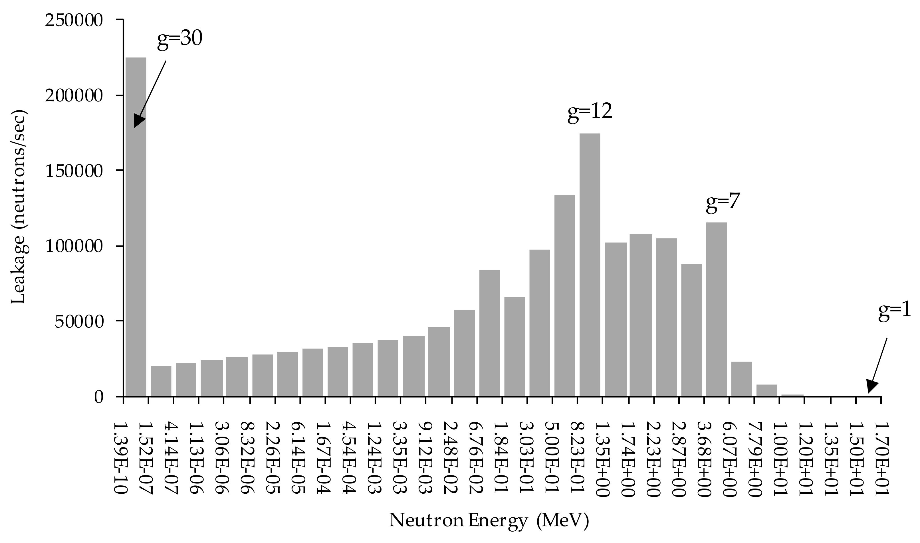

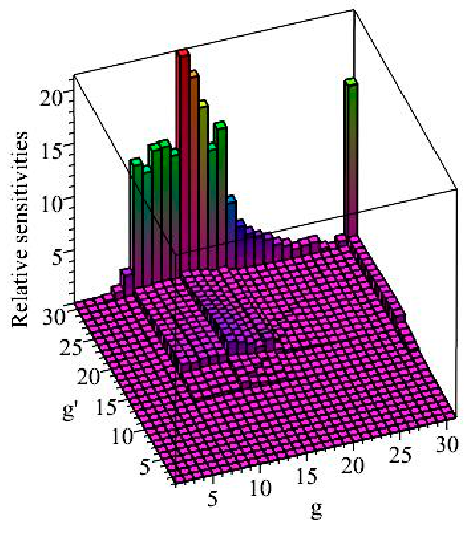

© 2019 by the authors. Licensee MDPI, Basel, Switzerland. This article is an open access article distributed under the terms and conditions of the Creative Commons Attribution (CC BY) license (http://creativecommons.org/licenses/by/4.0/).