Development of an Improved Model to Predict Building Thermal Energy Consumption by Utilizing Feature Selection

 ,
,
Abstract
1. Introduction
1.1. Background
1.2. Literature Review (Analysis of Previous Studies)
1.3. Study Objectives
2. Methodology
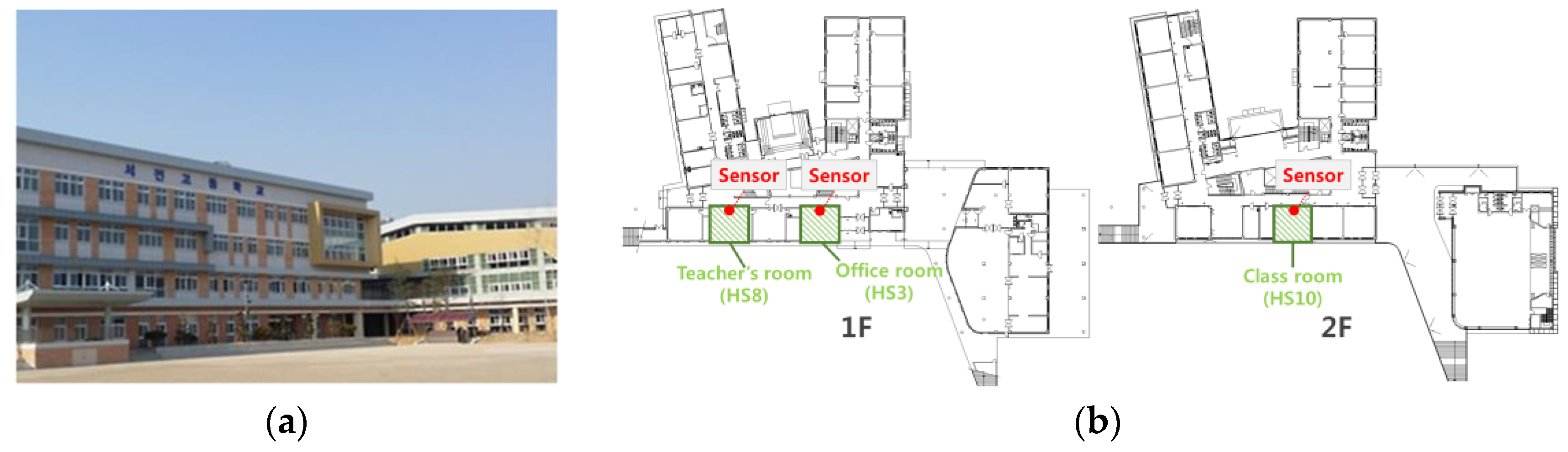
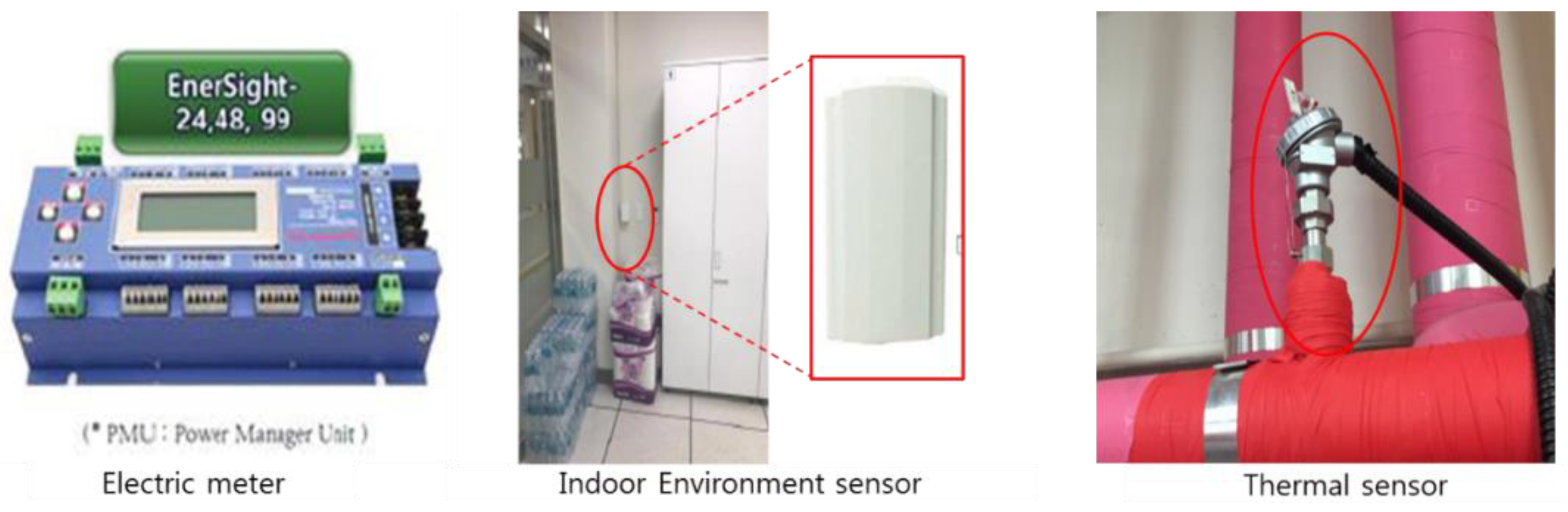
2.1. Building and Sensor Descriptions
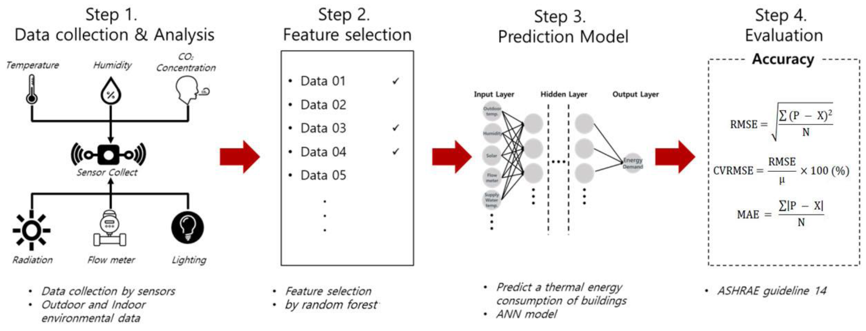
2.2. Prediction Process
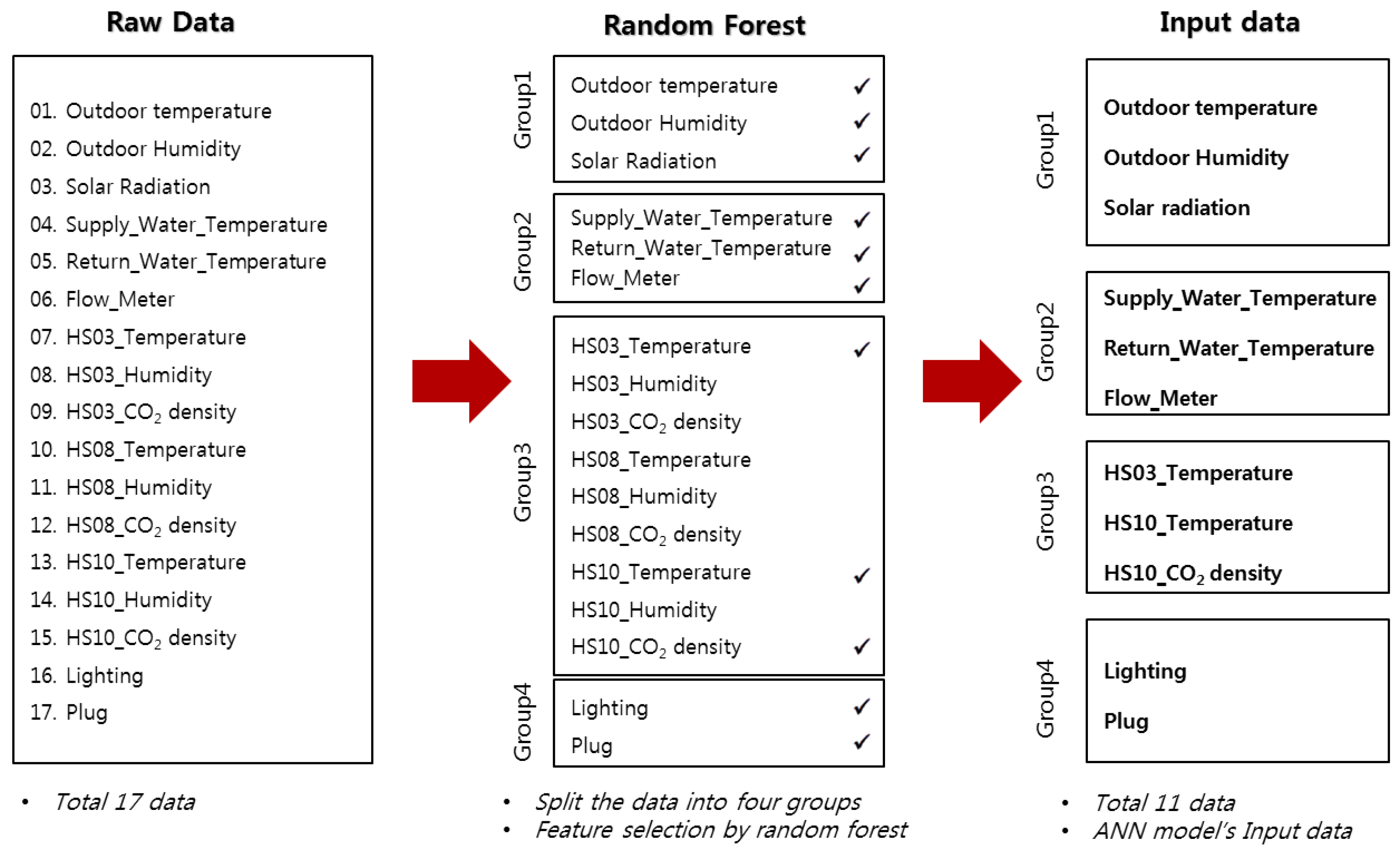
2.3. Feature Selection
2.4. ANN
2.5. Evaluation
3. Results
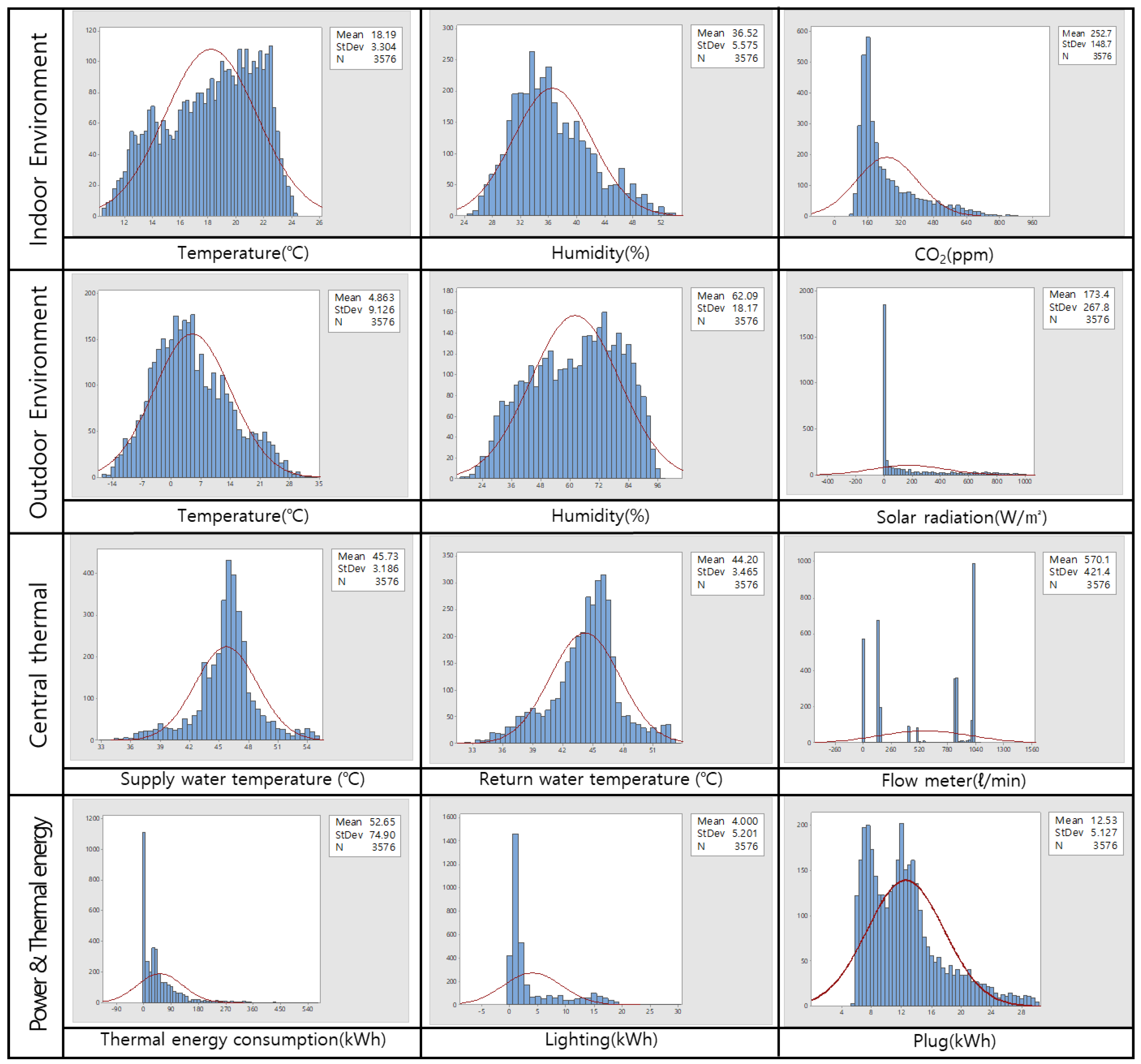
3.1. Overview of Data
3.2. Feature Selection by Random Forest
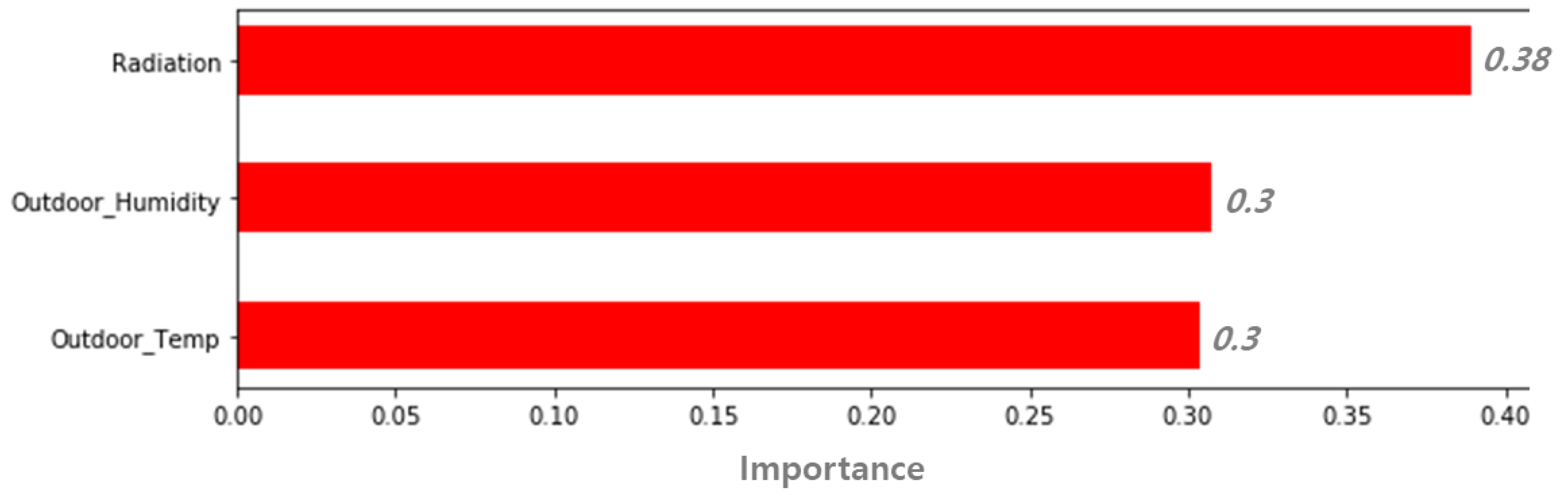
3.2.1. Outdoor Environment
3.2.2. Indoor Environment
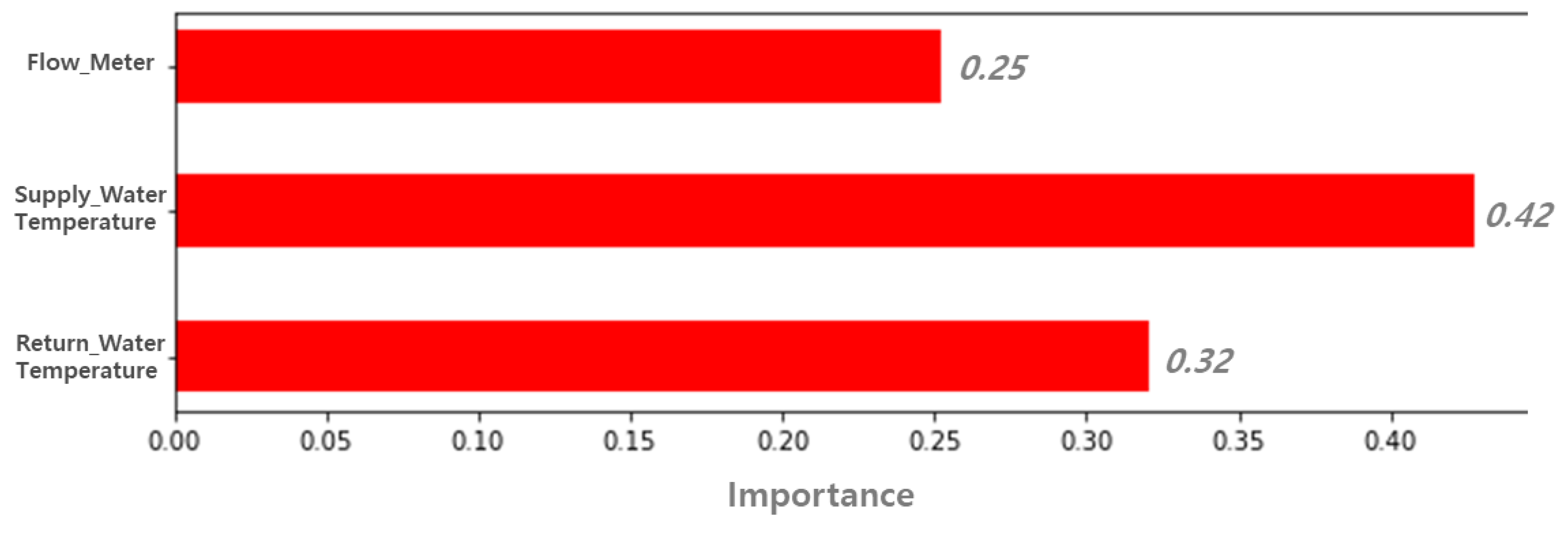
3.2.3. Central heating Supply Data
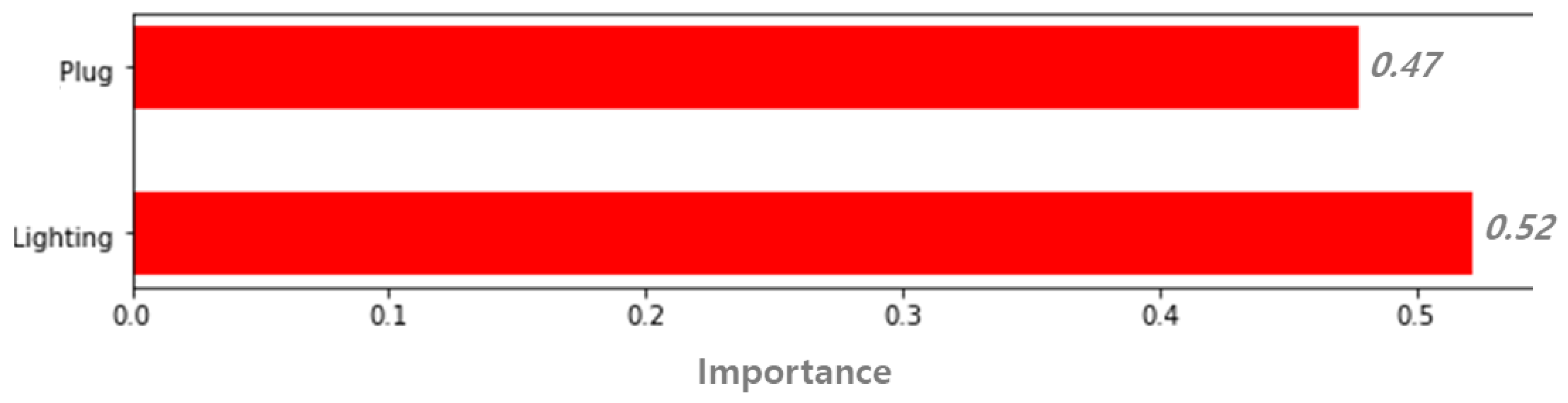
3.2.4. Electricity Energy Consumption Data
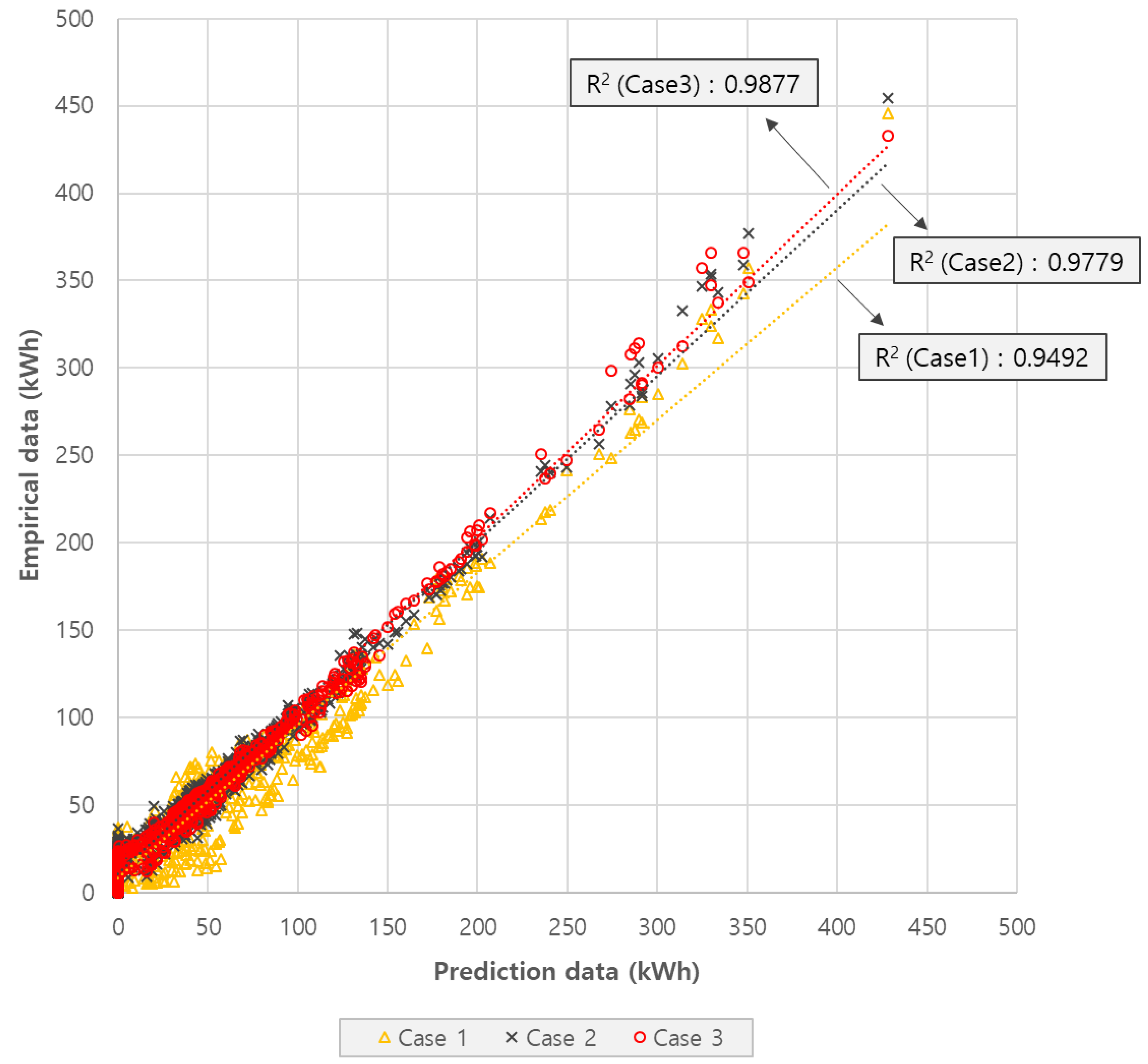
3.3. Prediction of Buildings’ Thermal Energy Consumption
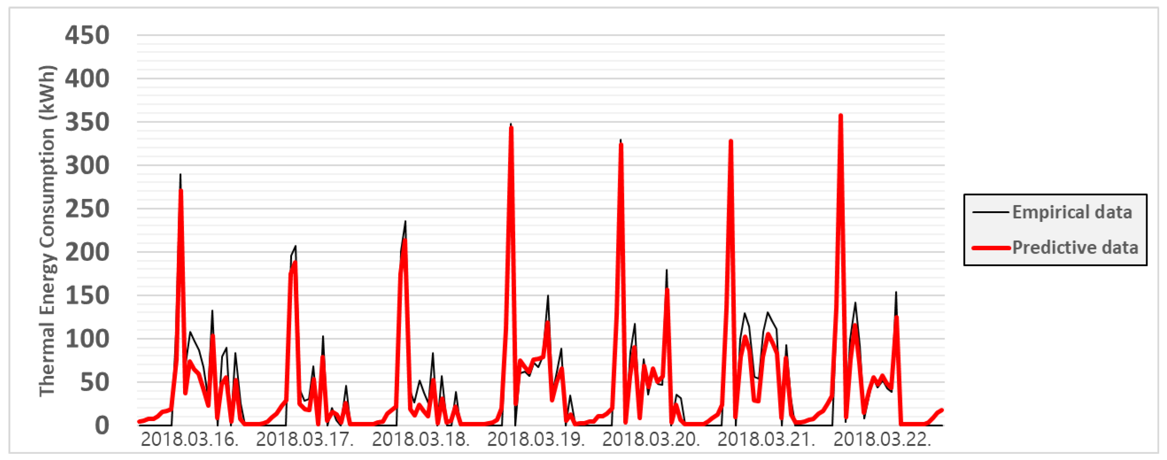
3.3.1. Case 1
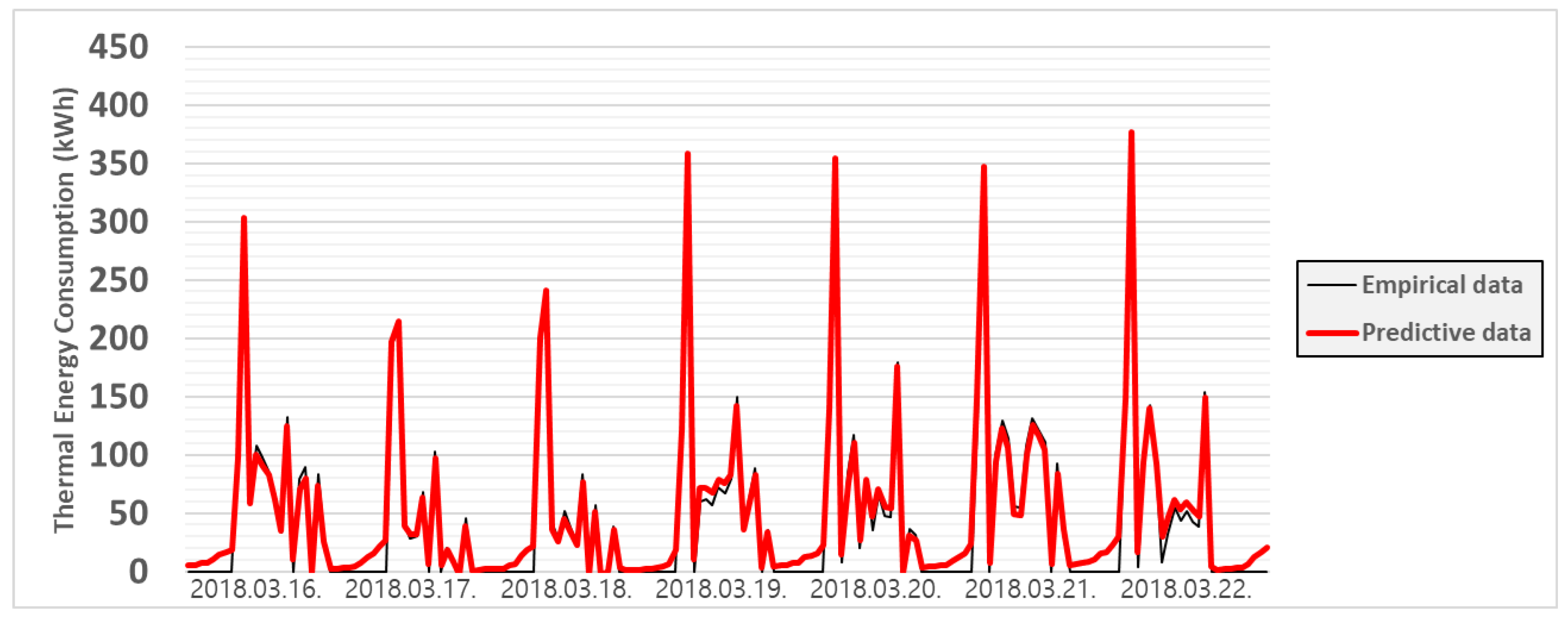
3.3.2. Case 2
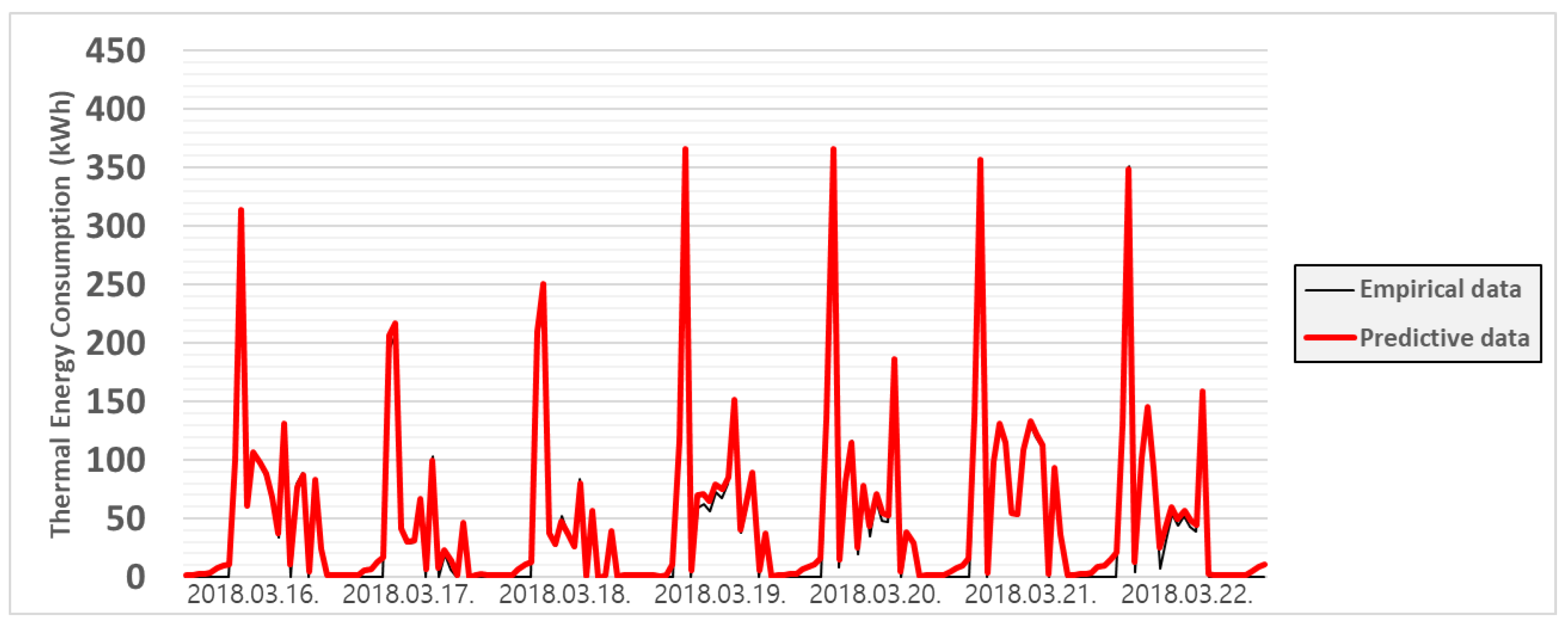
3.3.3. Case 3
4. Discussion
5. Conclusions
Author Contributions
Funding
Conflicts of Interest
References
- National Oceanic & Atmospheric Administration (NOAA). The NOAA Annual Greenhouse Gas Index (AGGI). Available online: https://www.esrl.noaa.gov/gmd/aggi/aggi.html (accessed on 8 July 2019).
- Kafle, S.; Parajuli, R.; Bhattarai, S.; Euh, S.H.; Kim, D.H. A review on energy systems and GHG emissions reduction plan and policy of the Republic of Korea: Past, present, and future. Renew. Sustain. Energy Rev. 2017, 73, 1123–1130. [Google Scholar] [CrossRef]
- Brophy, V.; Lewis, J.O. A Green Vitruvius: Principles and Practice of Sustainable Architectural Design, 2nd ed.; Routledge: Abingdon, UK, 2011; p. 32. [Google Scholar]
- IPCC. Fifth Assessment Report; IPCC: Geneva, Switzerland, 2014. [Google Scholar]
- Wu, H.J.; Yuan, Z.W.; Zhang, L.; Bi, J. Life cycle energy consumption and CO2 emission of an office building in China. Int. J. Life Cycle Assess. 2012, 17, 105–118. [Google Scholar] [CrossRef][Green Version]
- Torgal, F.P.; Mistretta, M.; Kaklauskas, A.; Granqvist, C.G.; Cabeza, L.F. Nearly Zero Energy Building Refurbishment: A Multidisciplinary Approach; Springer: Berlin, Germany, 2014. [Google Scholar]
- Pedersen, L.; Stang, J.; Ulseth, R. Load prediction method for heat and electricity demand in buildings for the purpose of planning for mixed energy distribution systems. Energy Build. 2008, 40, 1124–1134. [Google Scholar] [CrossRef]
- Ma, Y.; Borrelli, F.; Hencey, B.; Packard, A.; Bortoff, S. Model Predictive Control of thermal energy storage in building cooling systems. In Proceedings of the Joint 48th IEEE Conference on Decision and Control and 28th Chinese Control Conference, Shanghai, China, 15–18 December 2009. [Google Scholar]
- Dincer, I.; Dost, S.; Li, X. Performance analyses of sensible heat storage systems for thermal applications. Int. J. Energy Res. 1997, 21, 1157–1171. [Google Scholar] [CrossRef]
- Powell, K.M.; Sriprasad, A.; Cole, W.J.; Edgar, T.F. Heating, cooling, and electrical load forecasting for a large-scale district energy system. Energy 2014, 74, 877–885. [Google Scholar] [CrossRef]
- Idowu, S.; Saguna, S.; Åhlund, C.; Schelén, O. Applied machine learning: Forecasting heat load in district heating system. Energy Build. 2016, 133, 478–488. [Google Scholar] [CrossRef]
- Barak, S.; Sadegh, S.S. Forecasting energy consumption using ensemble ARIMA–ANFIS hybrid algorithm. Electr. Power Energy Syst. 2016, 82, 92–104. [Google Scholar] [CrossRef]
- Bedi, J.; Toshniwal, D. Deep learning framework to forecast electricity demand. Appl. Energy 2019, 238, 1312–1326. [Google Scholar] [CrossRef]
- Alfares, H.K.; Nazeeruddin, M. Electric load forecasting: Literature survey and classification of methods. Int. J. Syst. Sci. 2002, 33, 23–34. [Google Scholar] [CrossRef]
- Neto, A.H.; Fiorelli, F.A.S. Comparison between detailed model simulation and artificial neural network for forecasting building energy consumption. Energy Build. 2008, 40, 2169–2176. [Google Scholar] [CrossRef]
- Tso, G.K.F.; Yau, K.K.W. Predicting electricity energy consumption: A comparison of regression analysis, decision tree and neural networks. Energy 2007, 32, 1761–1768. [Google Scholar] [CrossRef]
- Hor, C.L.; Watson, S.J.; Majithia, S. Analyzing the impact of weather variables on monthly electricity demand. IEEE Trans. Power Syst. 2005, 20, 2078–2085. [Google Scholar] [CrossRef]
- Daut, M.A.M.; Hassan, M.Y.; Abdullah, H.; Rahman, H.A.; Abdullah, M.P.; Hussin, F. Building electrical energy consumption forecasting analysis using conventional and artificial intelligence methods: A review. Renew. Sustain. Energy Rev. 2017, 70, 1108–1118. [Google Scholar] [CrossRef]
- Almonacid, F.; Rus, C.; Pérez-Higueras, P.; Hontoria, L. Calculation of the energy provided by a PV generator. Comparative study: Conventional methods vs. artificial neural networks. Energy 2011, 36, 375–384. [Google Scholar] [CrossRef]
- Kialashaki, A.; Reisel, J.R. Development and validation of artificial neural network models of the energy demand in the industrial sector of the United States. Energy 2014, 76, 749–760. [Google Scholar] [CrossRef]
- Ekonomou, L. Greek long-term energy consumption prediction using artificial neural networks. Energy 2010, 35, 512–517. [Google Scholar] [CrossRef]
- Jovanović, R.Ž.; Sretenović, A.A.; Živković, B.D. Ensemble of various neural networks for prediction of heating energy consumption. Energy Build. 2015, 94, 189–199. [Google Scholar] [CrossRef]
- Ahmad, M.W.; Mourshed, M.; Rezgui, Y. Trees vs. Neurons: Comparison between random forest and ANN for high-resolution prediction of building energy consumption. Energy Build. 2017, 147, 77–89. [Google Scholar] [CrossRef]
- Abedinia, O.; Amjady, N.; Zareipour, H. A New Feature Selection Technique for Load and Price Forecast of Electrical Power Systems. IEEE Trans. Power Syst. 2017, 32, 62–74. [Google Scholar] [CrossRef]
- Jiang, P.; Liu, F.; Song, Y. A hybrid forecasting model based on date-framework strategy and improved feature selection technology for short-term load forecasting. Energy 2017, 119, 694–709. [Google Scholar] [CrossRef]
- Liu, Y.; Wang, W.; Ghadimi, N. Electricity load forecasting by an improved forecast engine for building level consumers. Energy 2017, 139, 18–30. [Google Scholar] [CrossRef]
- Zhao, H.-x.; Magoulès, F. Feature selection for support vector regression in the application of building energy prediction. In Proceedings of the 2011 IEEE 9th International Symposium on Applied Machine Intelligence and Informatics (SAMI), Smolenice, Slovakia, 27–29 January 2011; IEEE: Piscataway, NJ, USA. [Google Scholar]
- Cho, S.; Lee, J.; Baek, J.; Kim, G.S.; Leigh, S.B. Investigating Primary Factors Affecting Electricity Consumption in Non-Residential Buildings Using a Data-Driven Approach. Energies 2019, 12, 4046. [Google Scholar] [CrossRef]
- González-Vidal, A.; Jiménez, F.; Gómez-Skarmeta, A.F. A methodology for energy multivariate time series forecasting in smart buildings based on feature selection. Energy Build. 2019, 196, 71–82. [Google Scholar] [CrossRef]
- Yi, X.; Liu, F.; Liu, J.; Jin, H. Building a network highway for big data: Architecture and challenges. IEEE Netw. 2014, 28, 5–13. [Google Scholar] [CrossRef]
- Jang, J.; Baek, J.; Leigh, S.B. Prediction of optimum heating timing based on artificial neural network by utilizing BEMS data. J. Build. Eng. 2019, 22, 66–74. [Google Scholar] [CrossRef]
- Kim, M.H.; Kim, D.; Heo, J.; Lee, D.W. Energy performance investigation of net plus energy town: Energy balance of the Jincheon Eco-Friendly energy town. Renew. Energy 2020, 147, 1784–1800. [Google Scholar] [CrossRef]
- Kim, M.H.; Kim, D.; Heo, J.; Lee, D.W. Techno-economic analysis of hybrid renewable energy system with solar district heating for net zero energy community. Energy 2019, 187, 115916. [Google Scholar] [CrossRef]
- Deb, C.; Zhang, F.; Yang, J.; Lee, S.E.; Shah, K.W. A review on time series forecasting techniques for building energy consumption. Renew. Sustain. Energy Rev. 2017, 74, 902–924. [Google Scholar] [CrossRef]
- Nguyen, C.; Wang, Y.; Nguyen, H.N. Random forest classifier combined with feature selection for breast cancer diagnosis and prognostic. J. Biomed. Sci. Eng. 2013, 6, 551–560. [Google Scholar] [CrossRef]
- Breiman, L. Random Forests. Mach. Learn. 2001, 45, 5–32. [Google Scholar] [CrossRef]
- Zhang, Q.; Aires-de-Sousa, J. Random Forest Prediction of Mutagenicity from Empirical Physicochemical Descriptors. J. Chem. Inf. Modeling 2007, 47, 1–8. [Google Scholar] [CrossRef] [PubMed]
- Svetnik, V.; Liaw, A.; Tong, C.; Culberson, J.C.; Sheridan, R.P.; Feuston, B.P. Random Forest: A Classification and Regression Tool for Compound Classification and QSAR Modeling. J. Chem. Inf. Comput. Sci. 2003, 43, 1947–1958. [Google Scholar] [CrossRef] [PubMed]
- Han, H.; Guo, X.; Yu, H. Variable selection using Mean Decrease Accuracy and Mean Decrease Gini based on Random Forest. In Proceedings of the IEEE International Conference on Software Engineering and Service Sciences, ICSESS, Beijing, China, 24–26 November 2017. [Google Scholar]
- McCulloch, W.S.; Pitts, W. A logical calculus of the ideas immanent in nervous activity (reprinted from bulletin of mathematical biophysics. Bull. Math. Biol. 1990, 52, 99–115. [Google Scholar] [CrossRef] [PubMed]
- American Society of Heating, Refrigerating and Air-Conditioning Engineers (ASHRAE). ASHRAE guideline 14-2002 Measurement of Energy and Demand Saving: How to Determine What Was Really Saved by the Retrofit. In Proceedings of the Fifth International Conference for Enhanced Building Operations, Pittsburgh, Pennsylvania, 11–13 October 2005. [Google Scholar]


| Principal Use | Maximum Height | Total Floor Area | Building Area |
|---|---|---|---|
| High school | 14.7m | 10,431.85 m2 | 3871.92 m2 |
| Type | Nominal Operating Conditions | Value |
|---|---|---|
| Water Circulation Pump | Flow Rate(l/min) | 2200 |
| Head (m) | 10 | |
| Heat Exchanger | Capacity for heating (kcal/h) | 800,000 |
| Capacity for DHW (kcal/h) | 100,000 | |
| FCU | Capacity for heating (kcal/h) | 8450 |
| Flow Rate (l/min) | 18 |
| Office Room (HS3) | Teachers’ Room (HS8) | Classroom (HS10) | |
|---|---|---|---|
| The type of occupants | Support staff | Teachers | Students |
| The number of occupants | 6 | 6 | 23 |
| Area (m2) | 56 | 63 | 57 |
| Occupancy rate | 0.88 | 0.13 | 0.90 |
| Occupancy density (1·person/m2) | 0.11 | 0.10 | 0.40 |
| Installed FCU (EA) | 1 | 1 | 1 |
| No. | Category | Feature List | |
|---|---|---|---|
| 1 | Indoor environment data | Office (HS3) | Temperature (°C) Humidity (%) Concentration of CO2 (ppm) |
| Teachers’ room (HS8) | Temperature (°C) Humidity (%) Concentration of CO2 (ppm) | ||
| Classroom (HS10) | Temperature (°C) Humidity (%) Concentration of CO2 (ppm) | ||
| 2 | Outdoor environment data | Outdoor temperature (°C) Outdoor humidity (%) Solar radiation (W/m2) | |
| 3 | Central heating data | Return water temperature (°C) Supply water temperature (°C) Flow meter (L/min) | |
| 4 | Electricity energy data | Lighting (kWh) Plug load (kWh) | |
| 5 | Thermal energy consumption (kWh) | ||
| Experimental Sensor | Measuring Range | Accuracy | Resolution |
|---|---|---|---|
| Watt-hour sensor | 30–120 A | ±0.2% A, ±0.1% P | 0.01 kW |
| Temperature sensor | 0–50 °C | ±2 °C | 0.01 °C |
| Humidity sensor | 0–95% RH | ±2% RH | 0.01% RH |
| CO2 sensor | 0–10,000 ppm | ±5% measurement Value | 0.01 ppm |
| Calorimeter (Temperature) | 0–135 °C | ±5% measurement Value, ±1 °C | 2.5–50 °C |
| Calorimeter (Flow) | 10.0–250 m3/h | ±2 m3/h | 0.1 m3/h |
| Heating Hour | Occupants | Heating Duration | Set-Point Temperature |
|---|---|---|---|
| 07–22 | 590 people | Winter season (Nov.–Apr.) | 20 °C |
| Category | Parameter |
|---|---|
| Model | MLP (Multilayer Perceptron) Regressor |
| Activation function | ReLU |
| Learning rate | 0.01 |
| Momentum | 0.4 |
| Iterations | 1000 |
| The number of hidden layers | 5 |
| The number of hidden nodes | 128 |
| Accuracy | ASHRAE Guideline 14 | Case 1 | Case 2 | Case 3 |
|---|---|---|---|---|
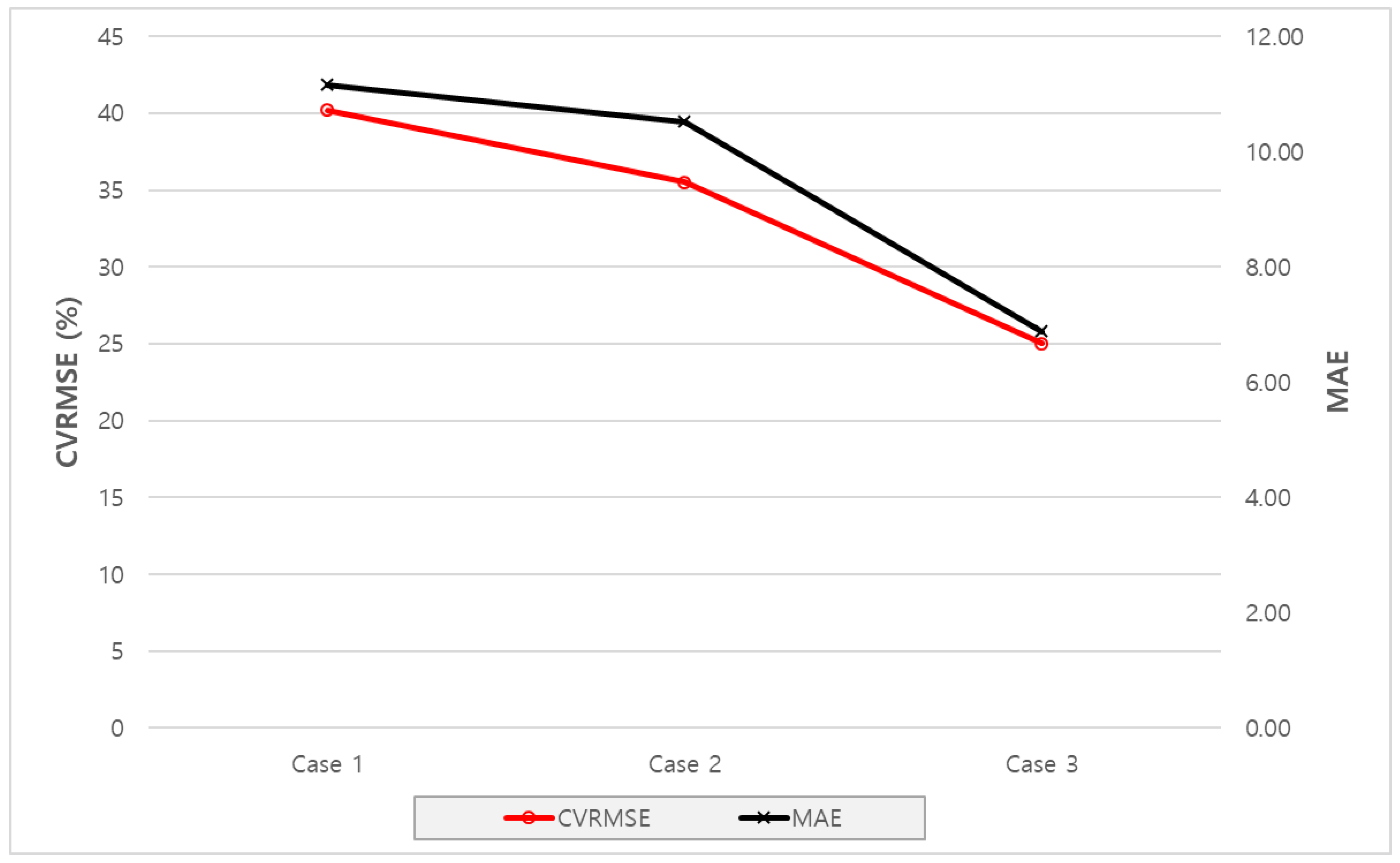
| CVRMSE | Criterion: Less than 30% | 40.19% | 35.52% | 25.01% |
| MAE | - | 11.16 | 10.52 | 6.88 |
© 2019 by the authors. Licensee MDPI, Basel, Switzerland. This article is an open access article distributed under the terms and conditions of the Creative Commons Attribution (CC BY) license (http://creativecommons.org/licenses/by/4.0/).
Share and Cite
Jang, J.; Lee, J.; Son, E.; Park, K.; Kim, G.; Lee, J.H.; Leigh, S.-B. Development of an Improved Model to Predict Building Thermal Energy Consumption by Utilizing Feature Selection. Energies 2019, 12, 4187. https://doi.org/10.3390/en12214187
Jang J, Lee J, Son E, Park K, Kim G, Lee JH, Leigh S-B. Development of an Improved Model to Predict Building Thermal Energy Consumption by Utilizing Feature Selection. Energies. 2019; 12(21):4187. https://doi.org/10.3390/en12214187
Chicago/Turabian StyleJang, Jihoon, Joosang Lee, Eunjo Son, Kyungyong Park, Gahee Kim, Jee Hang Lee, and Seung-Bok Leigh. 2019. "Development of an Improved Model to Predict Building Thermal Energy Consumption by Utilizing Feature Selection" Energies 12, no. 21: 4187. https://doi.org/10.3390/en12214187
APA StyleJang, J., Lee, J., Son, E., Park, K., Kim, G., Lee, J. H., & Leigh, S.-B. (2019). Development of an Improved Model to Predict Building Thermal Energy Consumption by Utilizing Feature Selection. Energies, 12(21), 4187. https://doi.org/10.3390/en12214187