An Optimisation Approach for Long-Term Industrial Investment Planning


Abstract
1. Introduction
- maintaining and/or refurbishing existing equipment to restore their efficiency;
- replacing and retiring obsolete equipment and production processes with the best available techniques; and
- using waste management measures such as insulation and sharing excess heat and material from one process to another.
2. State-Of-The-Art
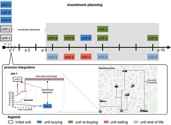
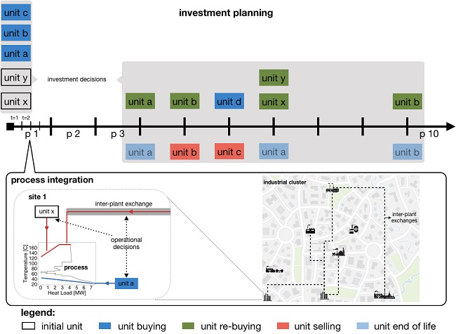
3. Method
3.1. Process Integration
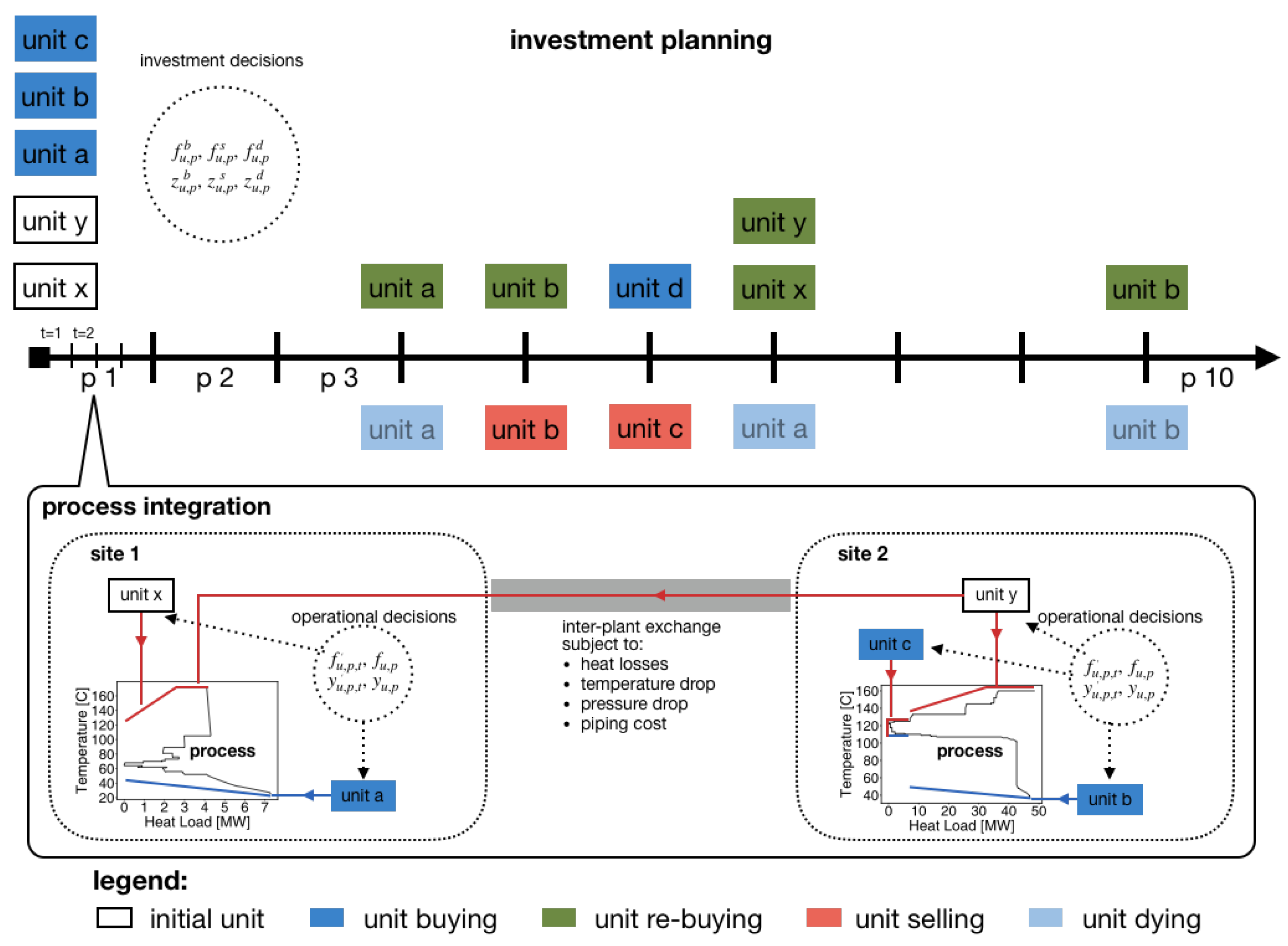
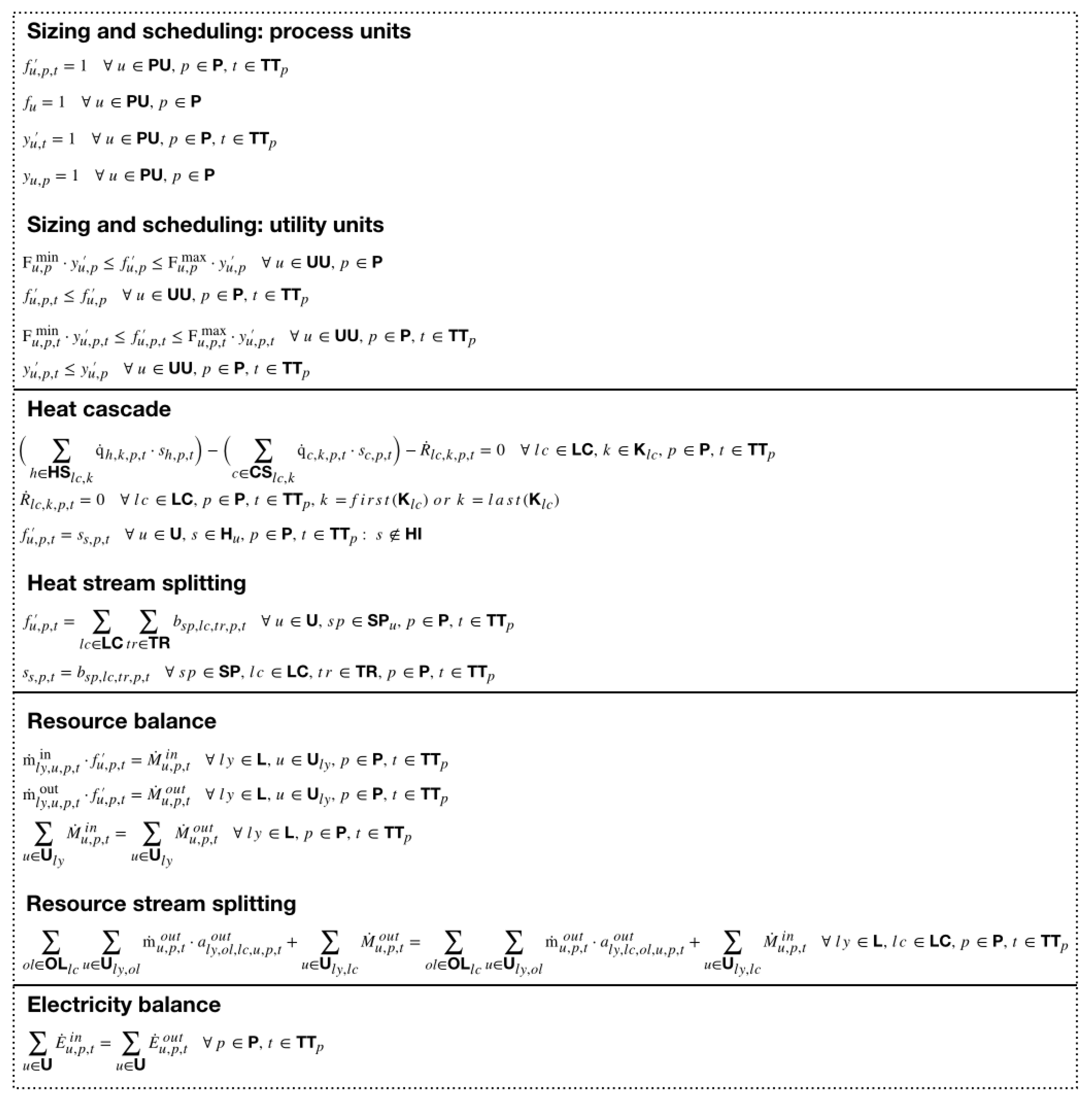
3.2. Investment Planning Model
- : The set of base case units. These units exist in the initial system in which the plants are operated business as usual. Thus, they do not need to be purchased initially.
- : The set of new units. This set consists of units that can potentially improve the efficiency of the plants (e.g., heat pumps), but currently do not exist on the sites. Therefore, they must be purchased before using them.
- : The set of investment units. This set includes base case and new units and it present to simplify the formulation, .
- A unit can exist only if it has a remaining life (Equation (15)).
- Only the existing units have a remaining life (Equation (16)).
- In the first period, the remaining life is equal to either the life span (for new units) or the difference between the life span and the initial age (base case units) (Equation (17)).
- In the other periods, the remaining life decreases compared from the previous period by one period. In addition, buying actions increase the remaining lifetime while selling decreases it (Equation (18)).
- A unit can be purchased again only after it is decommissioned (Equation (19)).
- A unit dies only if its lifetime in the previous period is one year (Equation (20)).
- A unit can be sold only if its lifetime in the previous period is two years or more (Equation (21)).
3.3. Economic Model
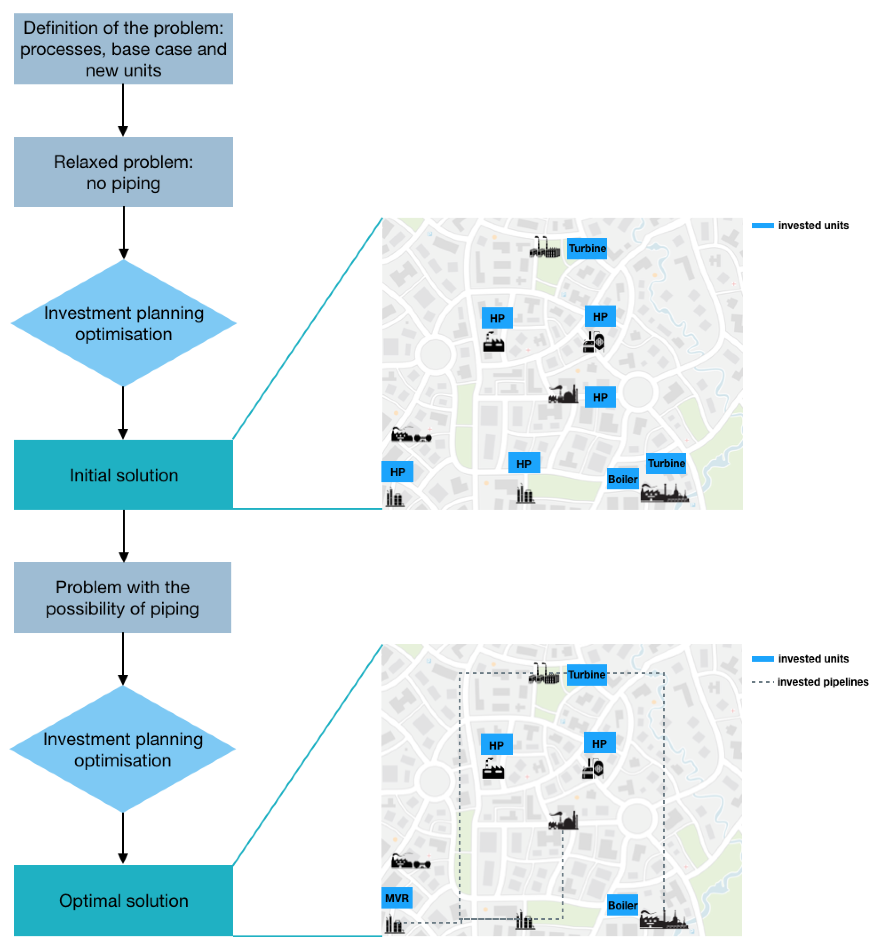
3.4. Solution Strategy
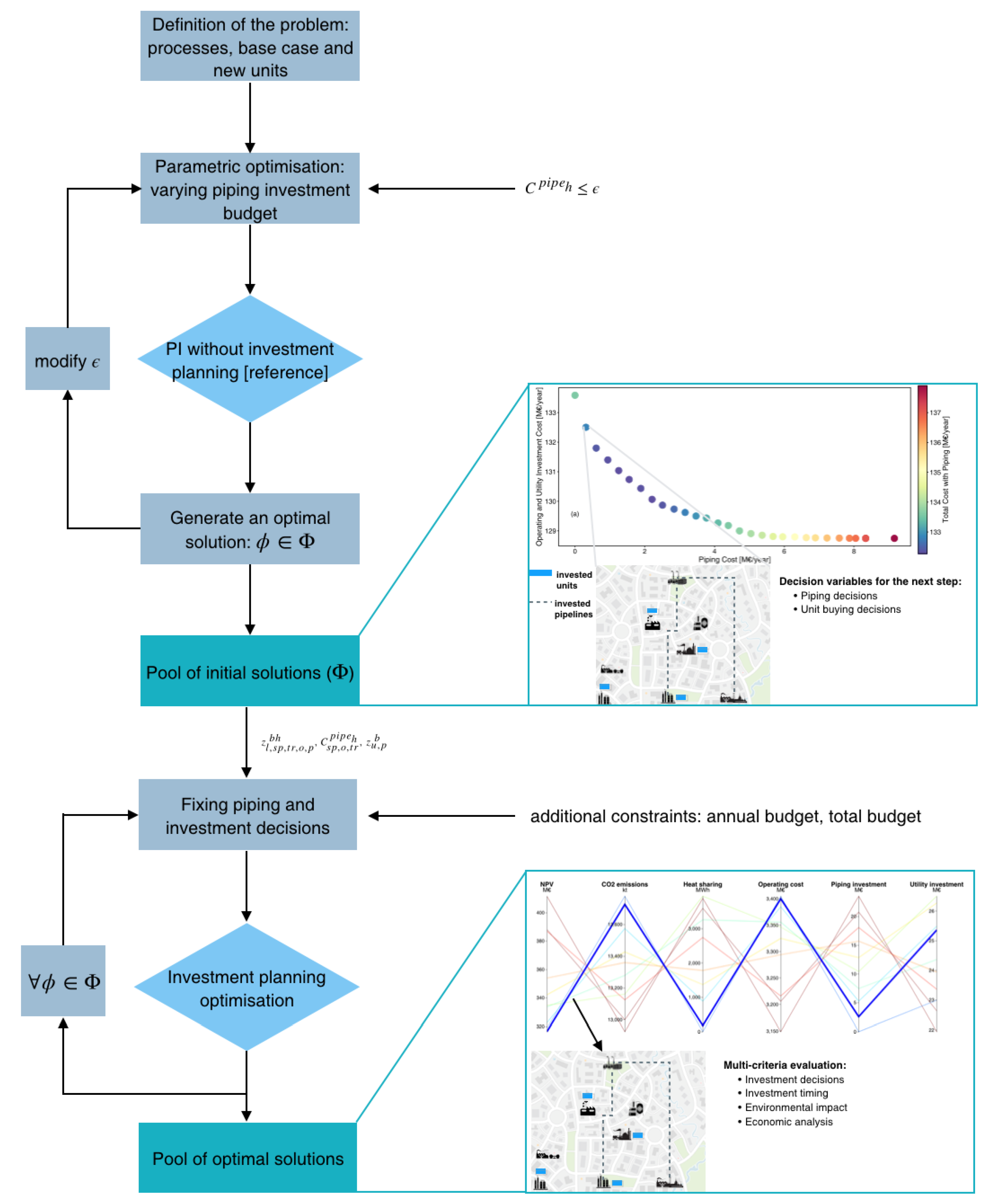
3.5. Systematic Generation of Multiple Solutions
4. Case Studies and Utility Systems
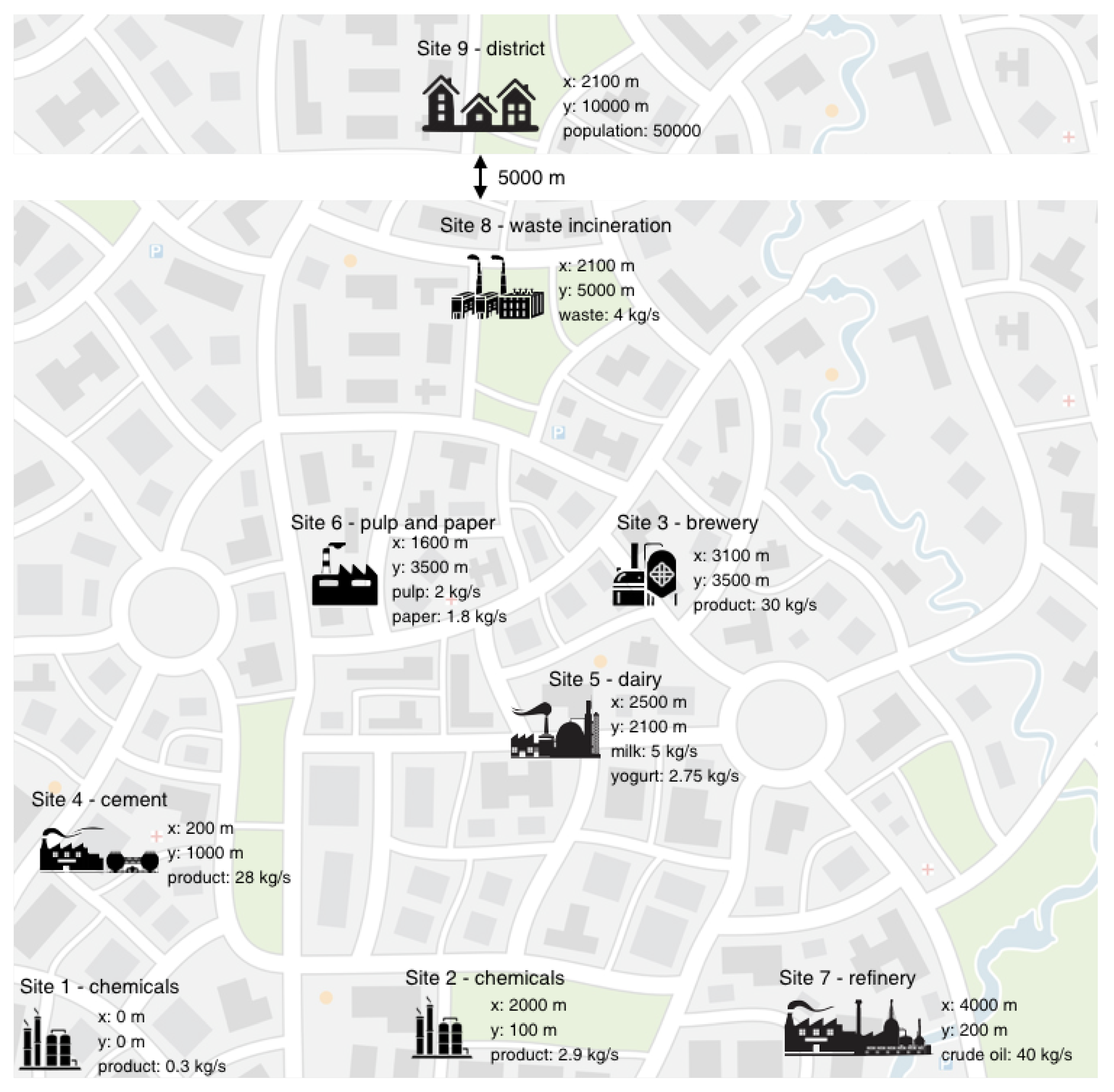
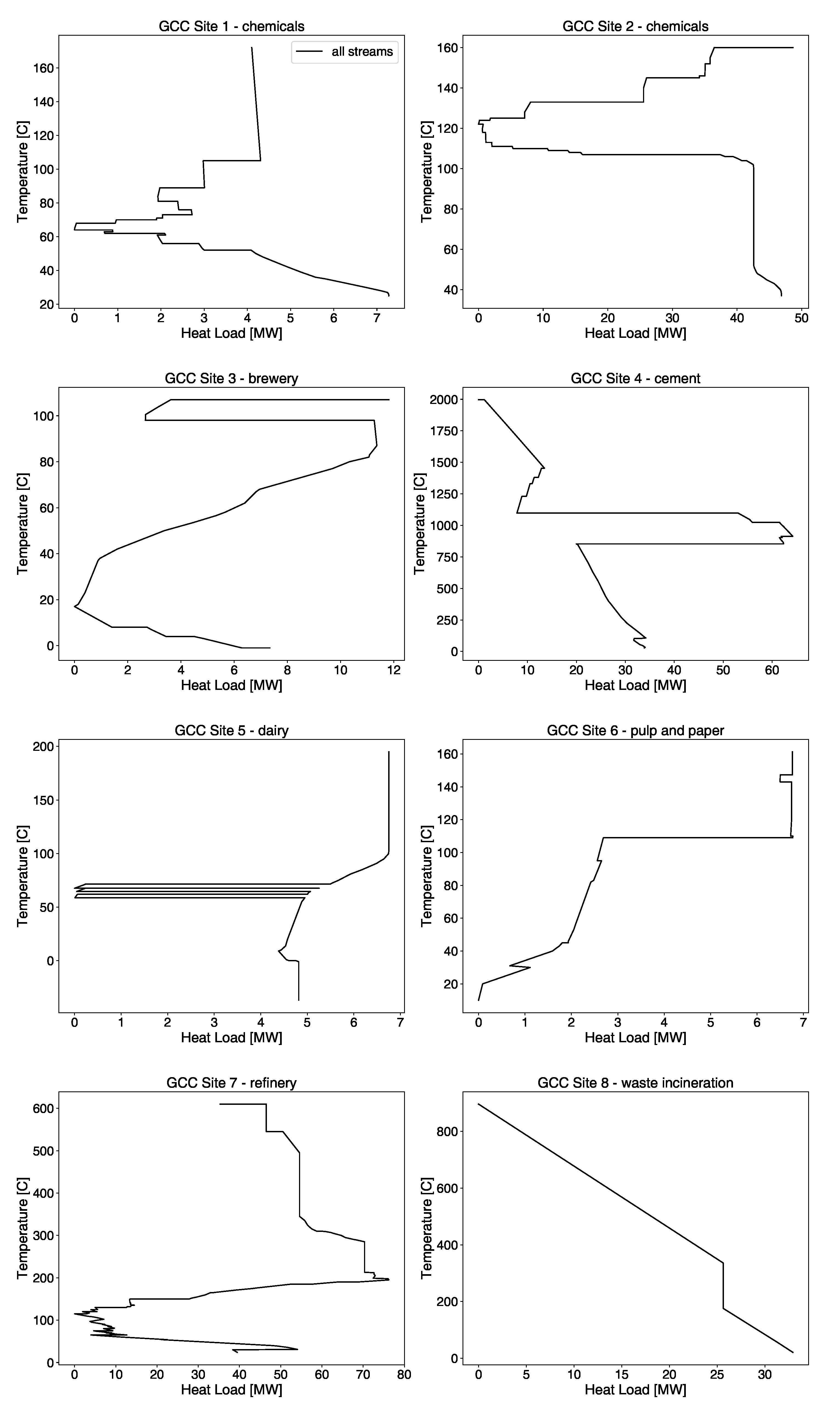
4.1. Utility Systems and Resources
- Site 4: The heating utility of the cement site is kiln, whereas cooling is carried out by air. Recovering the excess heat from the cement site and using it in other sites is not considered, as the technologies required are not mature enough. Thus, improvements in the utility system of the cement plant is not included in investment planning.
- Site 8: The waste incineration plant has a symbiosis potential by heat sharing with the other sites; however, improving the plant itself by integrating more efficient technologies is not studied in this work.
- Site 9: The district model is added in the case study to extend the potential of symbiosis. Except for sharing industrial excess heat with the district using a pipeline, improvements in the district utility system are not examined.
4.1.1. Existing Technologies on the Plants
Boilers
Steam Networks
Cooling Towers
4.1.2. Additional Technologies
Heat Pumps
Mechanical Vapor Recompression
Internal Combustion Engines
5. Results and Discussion
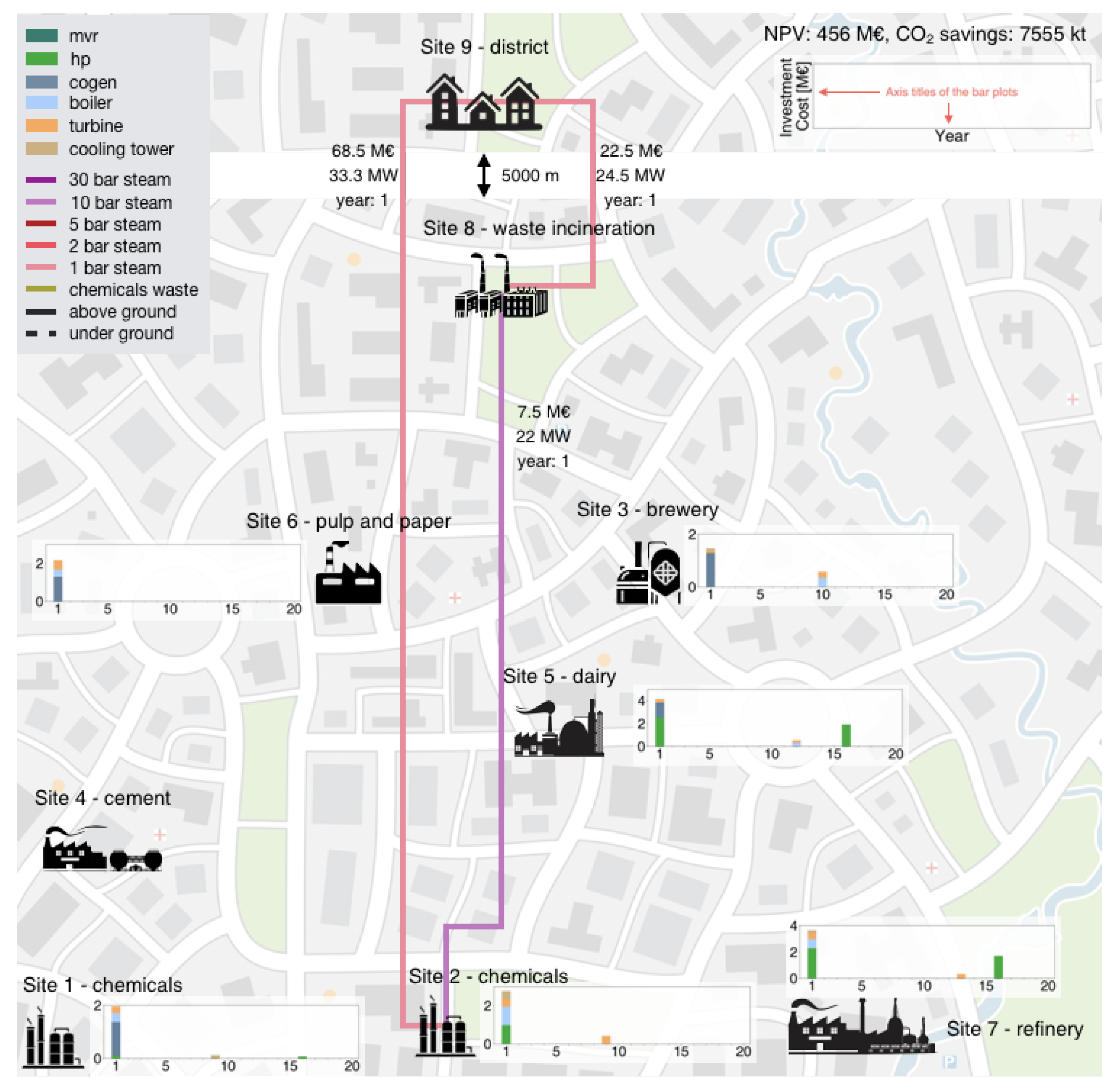
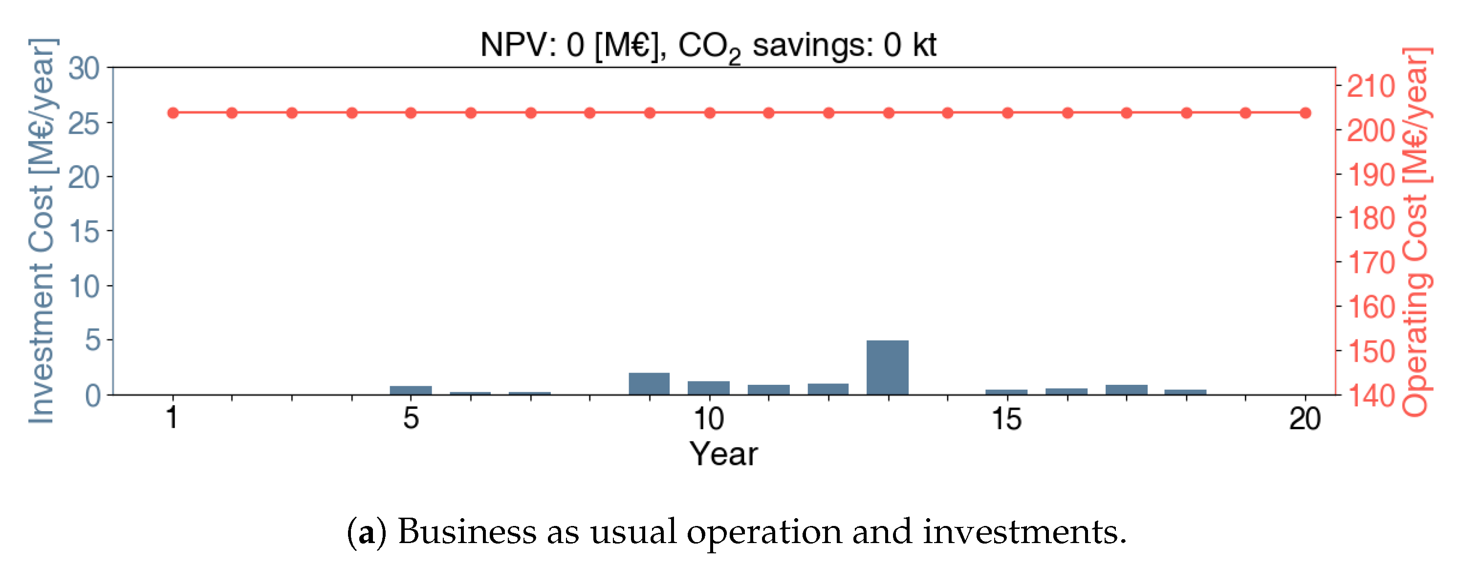
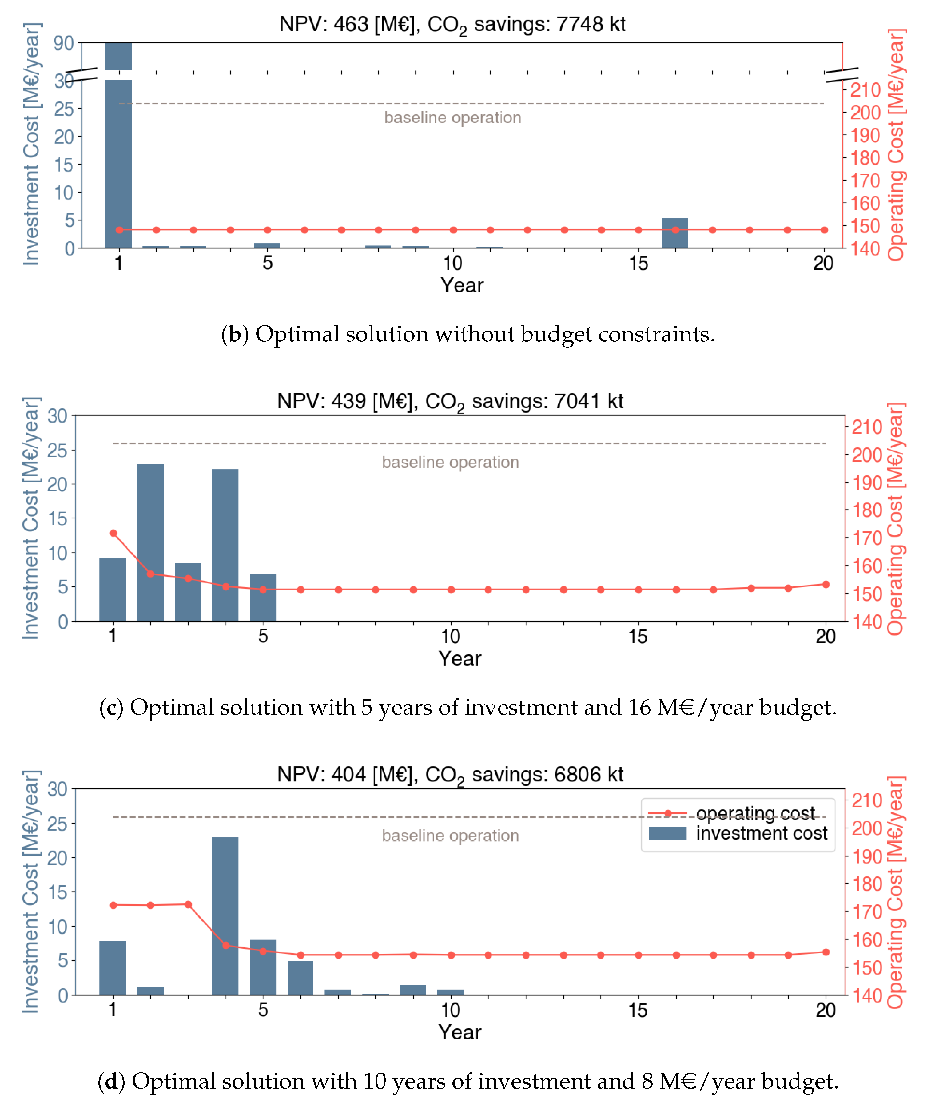
5.1. Optimal Investment Decisions without Budget Constraints
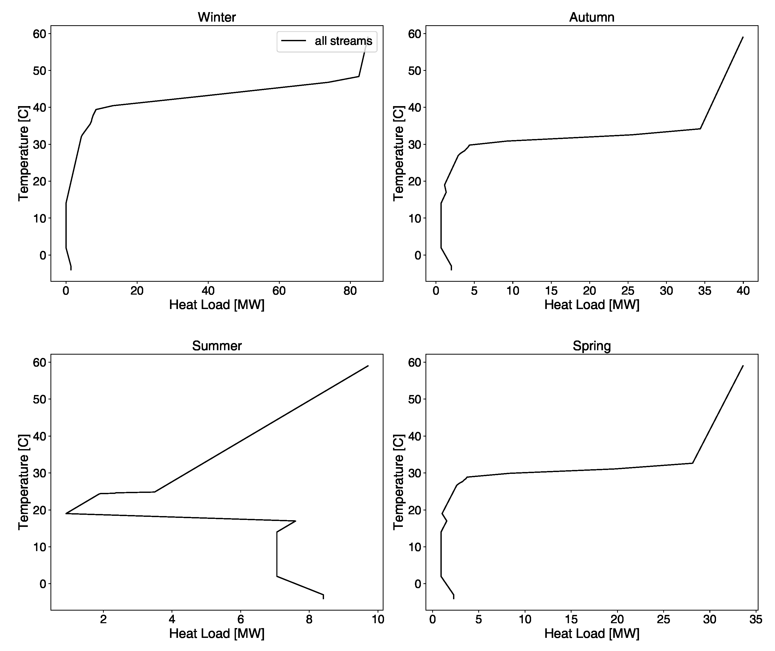
5.2. Impact of Seasonality in the Investment Decisions
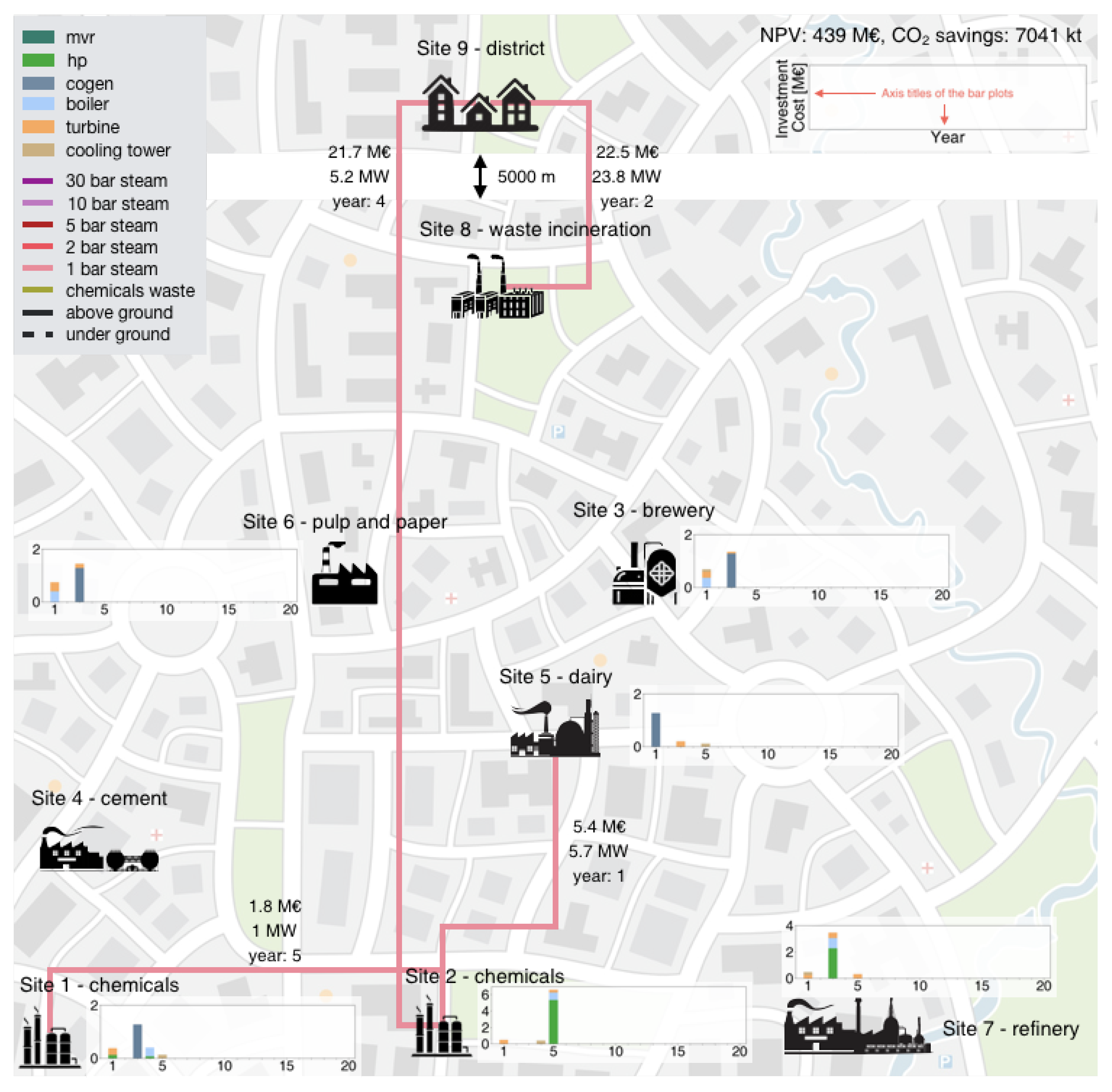
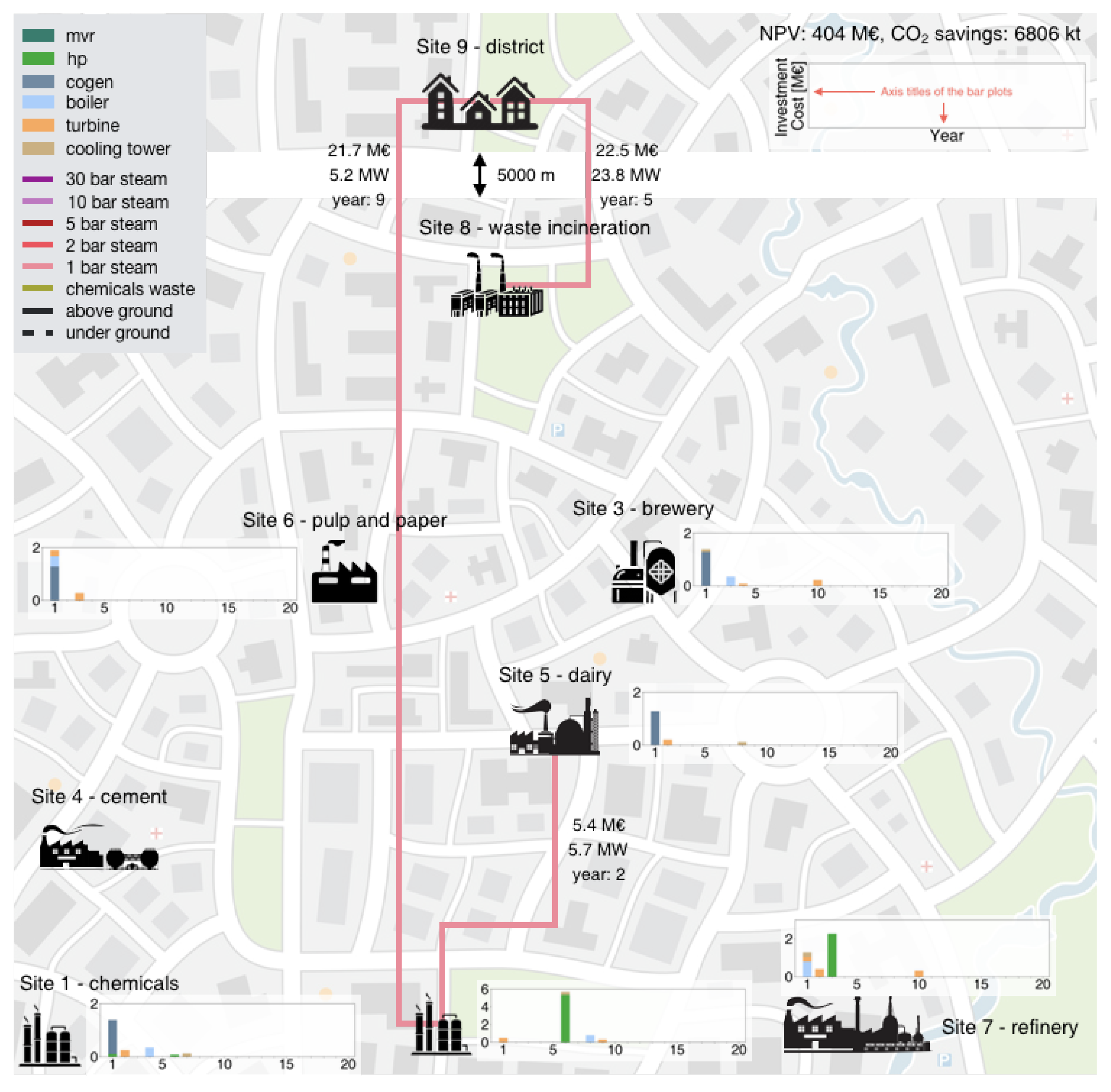
5.3. Budget and Investment Constraints
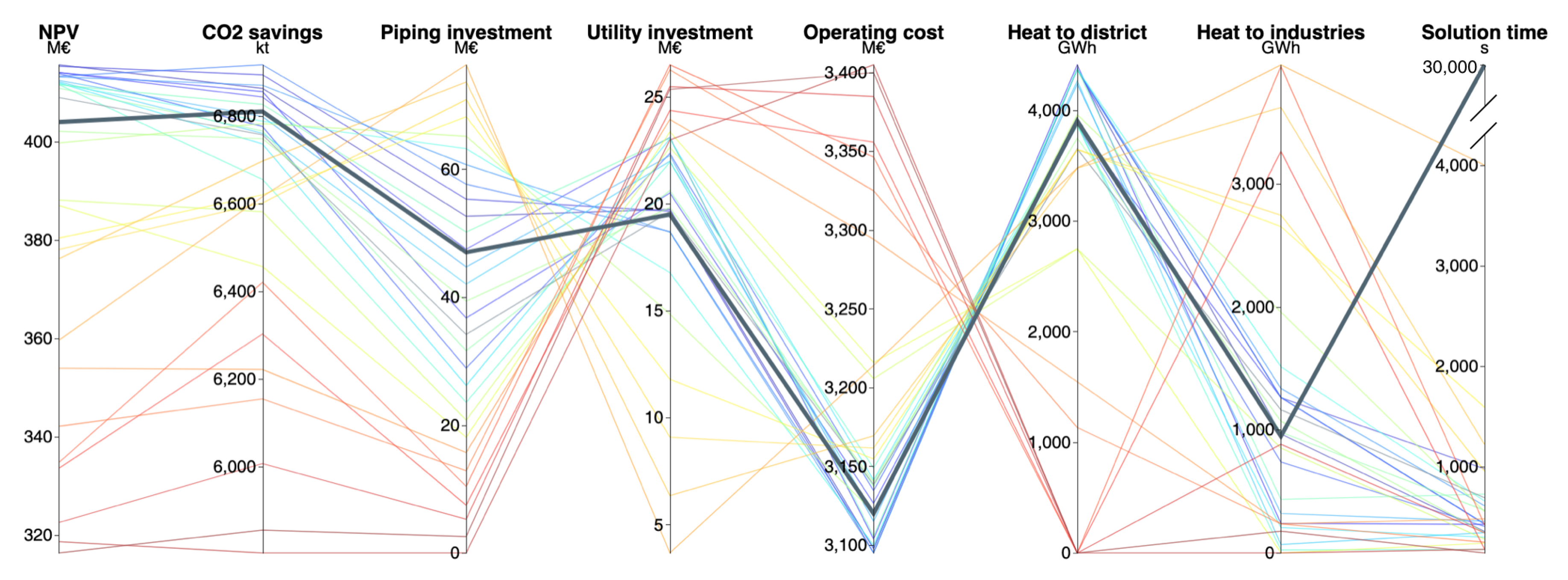
5.4. Multiple Scenarios for Investment
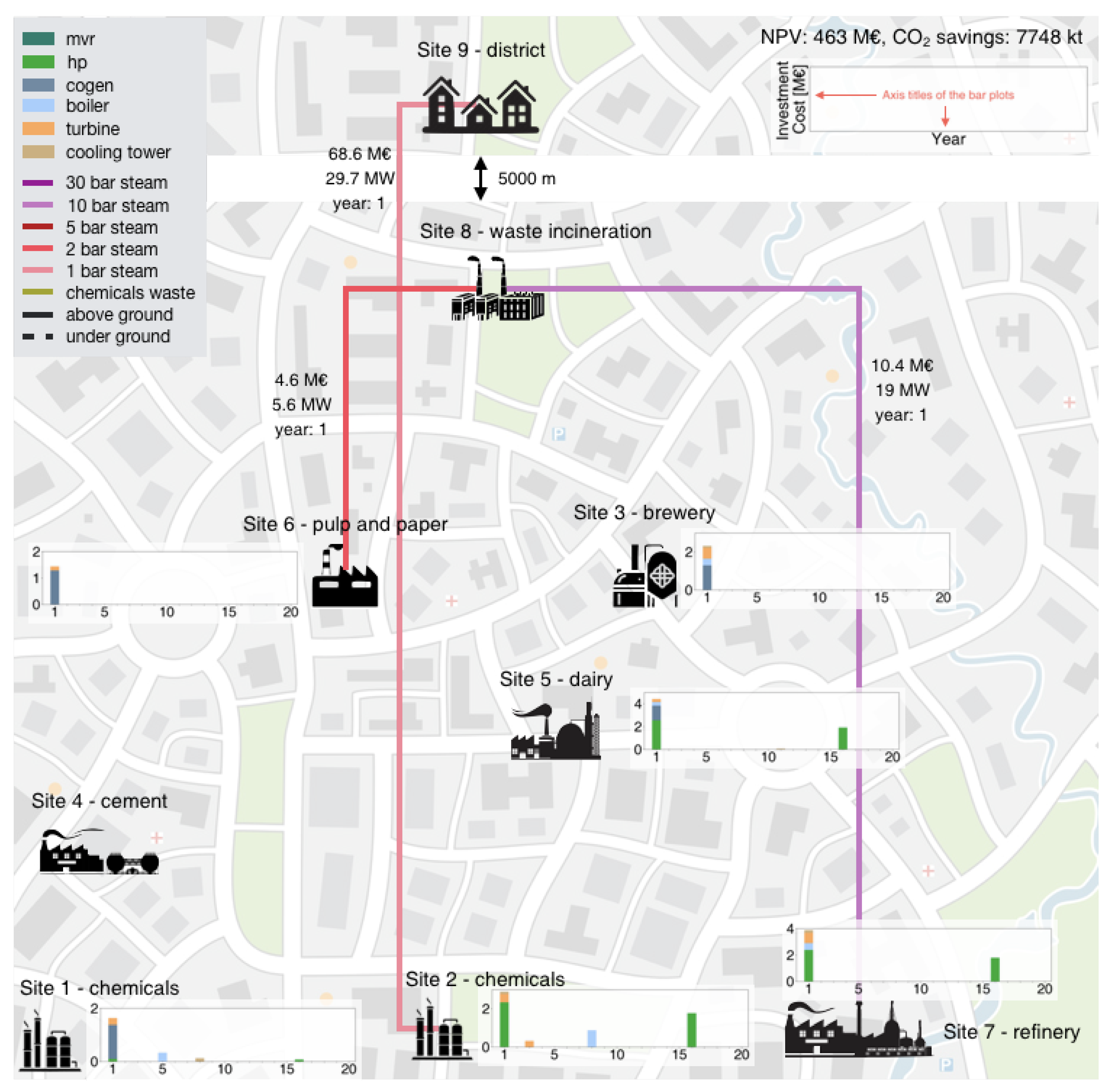
5.5. Comparison with Baseline
6. Conclusions
Author Contributions
Funding
Conflicts of Interest
Appendix A
Decommissioning Size Linearisation
Piping Investment Planning Model
Piping cost calculations

| Standard pipe size | 1 | 2 | 3 | 4 | 5 | 6 | 7 | 8 | 9 | 10 | 11 | 12 |
| Diameter (mm) | 20 | 40 | 80 | 100 | 200 | 300 | 400 | 500 | 600 | 800 | 1000 | 1500 |
| Specific cost (€/m) | 96 | 166 | 312 | 387 | 775 | 1180 | 1588 | 2008 | 2434 | 3304 | 4192 | 6474 |
Budget constraints
Materials and engineering cost linearisation
Selling and dying value linearisation
Linearisation of the max function
Grand composite curves of the sites


References
- International Energy Agency (IEA). World Energy Balances 2019; OECD Publishing: Paris, France, 2019; OCLC: 1013820838.
- International Energy Agency (IEA). CO2 Emissions from Fuel Combustion 2018; OECD Publishing: Paris, France, 2018; OCLC: 1013820838.
- Tanaka, K. Review of policies and measures for energy efficiency in industry sector. Energy Policy 2011, 39, 6532–6550. [Google Scholar] [CrossRef]
- International Energy Agency (IEA). Energy Technology Perspectives 2017; OECD Publishing: Paris, France, 2017.
- International Energy Agency (IEA). Energy Efficiency 2018; Technical Report; Organisation for Economic Co-operation and Development: Paris, France, 2018.
- Worrell, E.; Bernstein, L.; Roy, J.; Price, L.; Harnisch, J. Industrial energy efficiency and climate change mitigation. Energy Effic. 2009, 2, 109–123. [Google Scholar] [CrossRef]
- Walsh, C.; Thornley, P. Barriers to improving energy efficiency within the process industries with a focus on low grade heat utilisation. J. Clean. Prod. 2012, 23, 138–146. [Google Scholar] [CrossRef]
- Napp, T.; Gambhir, A.; Hills, T.; Florin, N.; Fennell, P. A review of the technologies, economics and policy instruments for decarbonising energy-intensive manufacturing industries. Renew. Sustain. Energy Rev. 2014, 30, 616–640. [Google Scholar] [CrossRef]
- Dhole, V.R.; Linnhoff, B. Total site targets for fuel, co-generation, emissions, and cooling. Comput. Chem. Eng. 1993, 17, S101–S109. [Google Scholar] [CrossRef]
- Papoulias, S.A.; Grossmann, I.E. A structural optimization approach in process synthesis—I. Comput. Chem. Eng. 1983, 7, 695–706. [Google Scholar] [CrossRef]
- Maréchal, F.; Kalitventzeff, B. Process integration: Selection of the optimal utility system. Comput. Chem. Eng. 1998, 22, S149–S156. [Google Scholar] [CrossRef]
- Kantor, I.; Betancourt, A.; Elkamel, A.; Fowler, M.; Almansoori, A. Generalized mixed-integer nonlinear programming modeling of eco-industrial networks to reduce cost and emissions. J. Clean. Prod. 2015, 99, 160–176. [Google Scholar] [CrossRef]
- Bagajewicz, M.; Rodera, H. Energy savings in the total site heat integration across many plants. Comput. Chem. Eng. 2000, 24, 1237–1242. [Google Scholar] [CrossRef]
- Becker, H.; Vuillermoz, A.; Maréchal, F. Heat pump integration in a cheese factory. Appl. Therm. Eng. 2012, 43, 118–127. [Google Scholar] [CrossRef]
- Porzio, G.F.; Colla, V.; Matarese, N.; Nastasi, G.; Branca, T.A.; Amato, A.; Fornai, B.; Vannucci, M.; Bergamasco, M. Process integration in energy and carbon intensive industries: An example of exploitation of optimization techniques and decision support. Appl. Therm. Eng. 2014, 70, 1148–1155. [Google Scholar] [CrossRef]
- Hansen, É.; Rodrigues, M.A.S.; Aragão, M.E.; de Aquim, P.M. Water and wastewater minimization in a petrochemical industry through mathematical programming. J. Clean. Prod. 2018, 172, 1814–1822. [Google Scholar] [CrossRef]
- Tilak, P.; El-Halwagi, M.M. Process integration of Calcium Looping with industrial plants for monetizing CO2 into value-added products. Carbon Resour. Convers. 2018, 1, 191–199. [Google Scholar] [CrossRef]
- Abikoye, B.; Čuček, L.; Isafiade, A.J.; Kravanja, Z. Integrated design for direct and indirect solar thermal utilization in low temperature industrial operations. Energy 2019, 182, 381–396. [Google Scholar] [CrossRef]
- Elsido, C.; Martelli, E.; Grossmann, I.E. A bilevel decomposition method for the simultaneous heat integration and synthesis of steam/organic Rankine cycles. Comput. Chem. Eng. 2019, 128, 228–245. [Google Scholar] [CrossRef]
- Kermani, M.; Kantor, I.; Wallerand, A.; Granacher, J.; Ensinas, A.; Maréchal, F. A Holistic Methodology for Optimizing Industrial Resource Efficiency. Energies 2019, 12, 1315. [Google Scholar] [CrossRef]
- Bütün, H.; Kantor, I.; Maréchal, F. Incorporating Location Aspects in Process Integration Methodology. Energies 2019, 12, 3338. [Google Scholar] [CrossRef]
- Bakirtzis, G.A.; Biskas, P.N.; Chatziathanasiou, V. Generation Expansion Planning by MILP considering mid-term scheduling decisions. Electr. Power Syst. Res. 2012, 86, 98–112. [Google Scholar] [CrossRef]
- Pereira, S.; Ferreira, P.; Vaz, A. Generation expansion planning with high share of renewables of variable output. Appl. Energy 2017, 190, 1275–1288. [Google Scholar] [CrossRef]
- Zhang, X.; Shahidehpour, M.; Alabdulwahab, A.; Abusorrah, A. Optimal Expansion Planning of Energy Hub With Multiple Energy Infrastructures. IEEE Trans. Smart Grid 2015, 6, 2302–2311. [Google Scholar] [CrossRef]
- Botterud, A.; Ilic, M.; Wangensteen, I. Optimal Investments in Power Generation Under Centralized and Decentralized Decision Making. IEEE Trans. Power Syst. 2005, 20, 254–263. [Google Scholar] [CrossRef]
- Bakken, B.H.; Skjelbred, H.I.; Wolfgang, O. eTransport: Investment planning in energy supply systems with multiple energy carriers. Energy 2007, 32, 1676–1689. [Google Scholar] [CrossRef]
- Mirzaesmaeeli, H.; Elkamel, A.; Douglas, P.; Croiset, E.; Gupta, M. A multi-period optimization model for energy planning with CO2 emission consideration. J. Environ. Manag. 2010, 91, 1063–1070. [Google Scholar] [CrossRef] [PubMed]
- Fripp, M. Switch: A Planning Tool for Power Systems with Large Shares of Intermittent Renewable Energy. Environ. Sci. Technol. 2012, 46, 6371–6378. [Google Scholar] [CrossRef]
- Cristóbal, J.; Guillén-Gosálbez, G.; Kraslawski, A.; Irabien, A. Stochastic MILP model for optimal timing of investments in CO2 capture technologies under uncertainty in prices. Energy 2013, 54, 343–351. [Google Scholar] [CrossRef]
- Cano, E.L.; Groissböck, M.; Moguerza, J.M.; Stadler, M. A strategic optimization model for energy systems planning. Energy Build. 2014, 81, 416–423. [Google Scholar] [CrossRef]
- Lambert, R.S.C.; Maier, S.; Shah, N.; Polak, J.W. Optimal phasing of district heating network investments using multistage stochastic programming. Int. J. Sustain. Energy Plan. Manag. 2016, 9. [Google Scholar] [CrossRef]
- Chakraborty, A.; Colberg, R.D.; Linninger, A.A. Plant-Wide Waste Management. 3. Long-Term Operation and Investment Planning under Uncertainty. Ind. Eng. Chem. Res. 2003, 42, 4772–4788. [Google Scholar] [CrossRef]
- Chakraborty, A.; Malcolm, A.; Colberg, R.D.; Linninger, A.A. Optimal waste reduction and investment planning under uncertainty. Comput. Chem. Eng. 2004, 28, 1145–1156. [Google Scholar] [CrossRef]
- Wickart, M.; Madlener, R. Optimal technology choice and investment timing: A stochastic model of industrial cogeneration vs. heat-only production. Energy Econ. 2007, 29, 934–952. [Google Scholar] [CrossRef]
- Sahinidis, N.; Grossmann, I.; Fornari, R.; Chathrathi, M. Optimization model for long range planning in the chemical industry. Comput. Chem. Eng. 1989, 13, 1049–1063. [Google Scholar] [CrossRef]
- Sahinidis, N.V.; Grossmann, I.E. Multiperiod investment model for processing networks with dedicated and flexible plants. Ind. Eng. Chem. Res. 1991, 30, 1165–1171. [Google Scholar] [CrossRef]
- Norton, L.C.; Grossmann, I.E. Strategic planning model for complete process flexibility. Ind. Eng. Chem. Res. 1994, 33, 69–76. [Google Scholar] [CrossRef]
- Jain, V.; Grossmann, I.E. Resource-Constrained Scheduling of Tests in New Product Development. Ind. Eng. Chem. Res. 1999, 38, 3013–3026. [Google Scholar] [CrossRef]
- Schmidt, C.W.; Grossmann, I.E. Optimization Models for the Scheduling of Testing Tasks in New Product Development. Ind. Eng. Chem. Res. 1996, 35, 3498–3510. [Google Scholar] [CrossRef]
- Maravelias, C.T.; Grossmann, I.E. Simultaneous Planning for New Product Development and Batch Manufacturing Facilities. Ind. Eng. Chem. Res. 2001, 40, 6147–6164. [Google Scholar] [CrossRef]
- Turton, R.; Bailie, R.C.; Whiting, W.B.; Shaeiwitz, J.A.; Bhattacharya, D. Analysis, Synthesis, and Design of Chemical Processes, 4th ed.; Prentice Hall: Upper Saddle River, NJ, USA, 2012. [Google Scholar]
- Gurobi Optimization, LLC. Gurobi Optimizer Reference Manual; Gurobi Optimization, LLC: Houston, TX, USA, 2019. [Google Scholar]
- CPLEX IBM ILOG. User’s Manual for CPLEX; IBM: Armonk, NY, USA, 2016. [Google Scholar]
- Haimes, Y.Y.; Lasdon, L.S.; Wismer, D.A. On a Bicriterion Formulation of the Problems of Integrated System Identification and System Optimization. IEEE Trans. Syst. Man Cybern. 1971, SMC-1, 296–297. [Google Scholar] [CrossRef]
- Kantor, I.; Wallerand, A.S.; Kermani, M.; Bütün, H.; Santecchia, A.; Norbert, R.; Cervo, H.; Arias, S.; Wolf, F.; Van Eetvelde, G.; et al. Thermal profile construction for energy-intensive industrial sectors. In Proceedings of the ECOS 2018—The 31st International Conference on Efficiency, Cost, Optimization, Simulation and Environmental Impact of Energy Systems, Guimaraes, Portugal, 17–22 June 2018. [Google Scholar]
- Bütün, H.; Kantor, I.; Maréchal, F. A heat integration method with multiple heat exchange interfaces. Energy 2018, 152, 476–488. [Google Scholar] [CrossRef]
- Suciu, R.; Kantor, I.; Bütün, H.; Maréchal, F. Geographically Parameterized Residential Sector Energy and Service Profile. Front. Energy Res. 2019, 7. [Google Scholar] [CrossRef]
- Loh, H. Process Equipment Cost Estimation Final Report; National Energy Technology Lab. (NETL): Pittsburgh, PA, USA, 2002; OCLC: 1096648453.
- Temple-Bird, C.; Kawohl, W.; Lenel, A.; Kaur, M. How to Plan and Budget for your Healthcate Technology; TALC: Hertfordshire, UK, 2005; OCLC: 1096648453. [Google Scholar]
- Maréchal, F.; Kalitventzeff, B. Targeting the optimal integration of steam networks: Mathematical tools and methodology. Comput. Chem. Eng. 1999, 23, S133–S136. [Google Scholar] [CrossRef]
- Ponce-Ortega, J.M.; Serna-González, M.; Jiménez-Gutiérrez, A. Optimization model for re-circulating cooling water systems. Comput. Chem. Eng. 2010, 34, 177–195. [Google Scholar] [CrossRef]
- Nussbaumer, T.; Thalmann, S. Influence of system design on heat distribution costs in district heating. Energy 2016, 101, 496–505. [Google Scholar] [CrossRef]
- Kwak, D.H.; Binns, M.; Kim, J.K. Integrated design and optimization of technologies for utilizing low grade heat in process industries. Appl. Energy 2014, 131, 307–322. [Google Scholar] [CrossRef]
- Alva-Argáez, A.; Kokossis, A.C.; Smith, R. The design of water-using systems in petroleum refining using a water-pinch decomposition. Chem. Eng. J. 2007, 128, 33–46. [Google Scholar] [CrossRef]
- Nordman, R.; Berntsson, T. Use of advanced composite curves for assessing cost-effective HEN retrofit II. Case studies. Appl. Therm. Eng. 2009, 29, 282–289. [Google Scholar] [CrossRef]
- Persson, J.; Berntsson, T. Influence of short-term variations on energy-saving opportunities in a pulp mill. J. Clean. Prod. 2010, 18, 935–943. [Google Scholar] [CrossRef]


| Location | F (-) | c (k€) | c (k€) | LI (years) |
|---|---|---|---|---|
| Site 1 | 7 | 388 | 13 | 16 |
| Site 2 | 62 | 388 | 13 | 12 |
| Site 3 | 30 | 388 | 13 | 11 |
| Site 5 | 19 | 388 | 13 | 9 |
| Site 6 | 11 | 388 | 13 | 6 |
| Site 7 | 190 | 388 | 13 | 8 |
| Location | Inlet (bar) | Outlet (bar) | F (-) | c (k€) | c (k€) | LI (years) |
|---|---|---|---|---|---|---|
| Site 1 | 45 | 24 | 1.3 | 64 | 22 | 16 |
| Site 1 | 45 | 8 | 1.6 | 153 | 19 | 16 |
| Site 2 | 45 | 24 | 12.2 | 64 | 22 | 12 |
| Site 2 | 45 | 8 | 12.4 | 153 | 19 | 12 |
| Site 3 | 45 | 2 | 13 | 232 | 16 | 11 |
| Site 5 | 45 | 2 | 8 | 232 | 16 | 9 |
| Site 6 | 45 | 4 | 5 | 195 | 18 | 6 |
| Site 7 | 45 | 24 | 24 | 64 | 22 | 8 |
| Site 7 | 45 | 8 | 14 | 153 | 19 | 8 |
| Site 7 | 45 | 4 | 50 | 195 | 18 | 8 |
| Location | F (-) | c (k€) | c (k€) | LI (years) |
|---|---|---|---|---|
| Site 1 | 9 | 82 | 13 | 15 |
| Site 2 | 57 | 82 | 13 | 10 |
| Site 3 | 22 | 82 | 13 | 3 |
| Site 5 | 5 | 82 | 13 | 14 |
| Site 6 | 2 | 82 | 13 | 6 |
| Site 7 | 150 | 82 | 13 | 4 |
| Location | c (k€) | c (k€) | LI (years) |
|---|---|---|---|
| Site 1 | 26 | 52 | 15 |
| Site 2 | 556 | 216 | 15 |
| Site 5 | 270 | 454 | 15 |
| Site 7 | 305 | 217 | 15 |
| Location | c (k€) | c (k€) | LI (years) |
|---|---|---|---|
| Site 1 | 36 | 317 | 15 |
| Site 3 | 151 | 261 | 15 |
| Site 6 | 9 | 38 | 15 |
© 2019 by the authors. Licensee MDPI, Basel, Switzerland. This article is an open access article distributed under the terms and conditions of the Creative Commons Attribution (CC BY) license (http://creativecommons.org/licenses/by/4.0/).
Share and Cite
Bütün, H.; Kantor, I.; Maréchal, F. An Optimisation Approach for Long-Term Industrial Investment Planning. Energies 2019, 12, 4076. https://doi.org/10.3390/en12214076
Bütün H, Kantor I, Maréchal F. An Optimisation Approach for Long-Term Industrial Investment Planning. Energies. 2019; 12(21):4076. https://doi.org/10.3390/en12214076
Chicago/Turabian StyleBütün, Hür, Ivan Kantor, and François Maréchal. 2019. "An Optimisation Approach for Long-Term Industrial Investment Planning" Energies 12, no. 21: 4076. https://doi.org/10.3390/en12214076
APA StyleBütün, H., Kantor, I., & Maréchal, F. (2019). An Optimisation Approach for Long-Term Industrial Investment Planning. Energies, 12(21), 4076. https://doi.org/10.3390/en12214076