A Novel Fault Diagnosis Method for Power Transformer Based on Dissolved Gas Analysis Using Hypersphere Multiclass Support Vector Machine and Improved D–S Evidence Theory

Abstract

Power transformers are important equipment in power systems and their reliability directly concerns the safety of power networks. Dissolved gas analysis (DGA) has shown great potential for detecting the incipient fault of oil-filled power transformers. In order to solve the misdiagnosis problems of traditional fault diagnosis approaches, a novel fault diagnosis method based on hypersphere multiclass support vector machine (HMSVM) and Dempster–Shafer (D–S) Evidence Theory (DET) is proposed. Firstly, proper gas dissolved in oil is selected as the fault characteristic of power transformers. Secondly, HMSVM is employed to diagnose transformer fault with selected characteristics. Then, particle swarm optimization (PSO) is utilized for parameter optimization. Finally, DET is introduced to fuse three different fault diagnosis methods together, including HMSVM, hybrid immune algorithm (HIA), and kernel extreme learning machine (KELM). To avoid the high conflict between different evidences, in this paper, a weight coefficient is introduced for the correction of fusion results. Results indicate that the fault diagnosis based on HMSVM has the highest probability to identify transformer faults among three artificial intelligent approaches. In addition, the improved D–S evidence theory (IDET) combines the advantages of each diagnosis method and promotes fault diagnosis accuracy.

1. Introduction

As the equipment for transferring electric energy, power transformers occupy an important position in the power system. Their operation state is directly related to the security and stability of the power system [1]. Dissolved Gas Analysis (DGA) is one of the most effective measures to monitor the safe operation of oil-immersed transformers, which can detect the latent faults in the equipment as early as possible [2]. However, the mechanism of transformer fault gas generation is complex, and the mapping relationship between dissolved gas and fault types is relatively vague, which makes it difficult for transformer fault diagnosis [3].

In recent years, various kinds of intelligent algorithms have been applied to transformer fault diagnosis. Support vector machine (SVM) uses hyperplane in high-dimensional kernel feature space to realize classification, which has global optimum and strong generalization ability [4]. At present, SVM has been widely used in the transformer fault diagnosis field [5,6,7,8,9]. However, for samples with uneven state distribution, the hyperplane model of SVM is difficult to classify accurately. In addition, SVM has some limitations in practical applications because of its inherent binary classification attribute, high complexity, and time-consuming calculation.

Hypersphere support vector machine (HSSVM) is based on the theory of SVM. It was first proposed by Scholkopf to replace the hyperplane of SVM with a hypersphere for pattern recognition [10]. Unlike hyperplanar SVM, HSSVM can not only separate two classes of samples, but also divide the sample space into two parts with different status, which can separate the samples distributed in a certain region well [11]. For k-classification, HSSVM only needs to compute k quadratic programming. Compared with the indirect classification of SVM, HSSVM needs fewer quadratic constraints and shorter training and testing time [12]. Ai proposed a novel binary classifier named twin-hypersphere SVM. The algorithm not only inherits good properties, but also gives a more robust description for the dataset. Experimental results on synthetic and publicly available benchmark datasets show the excellent performance in terms of classification accuracy and learning time [13]. In order to solve the multi-classification problems of HSSVM, Zhu put forward a theory of multiclass SVM with a spherical structure [14]. The kernel method was applied to spherical classification in this work. A new hypersphere multi-class support vector machine was proposed in [15] and applied in text classification, but the parameter setting of the method was not explained further. In [16], hypersphere multiclass SVM (HMSVM) was used for partial discharge pattern recognition using dispersion entropy as PD features. Recognition results verified the effectiveness of the method. In this paper, particle swarm optimization (PSO) [17,18] is used to optimize the parameters of HMSVM, and the optimized HMSVM algorithm is applied to transformer fault diagnosis.

Due to the ambiguous relationship between transformer fault phenomena and fault causes, it results in great differences in the effect of different methods on transformer fault diagnosis with different states [19]. Dempster–Shafer evidence theory (DET) is a theory for studying uncertainty [20]. It provides an effective method for reasoning and fusion of uncertain information from multiple data sources. In recent years, DET has been applied in many fields, such as medical diagnosis, military affairs, fault diagnosis, and so on [21,22,23,24,25]. However, when there is a high conflict between evidences, Dempster’s synthetic rule has a big defect. The synthetic result may be contrary to the reality [26]. In order to solve the problem of high conflict between evidence, the weight coefficient is introduced to adjust basic probability assignment (BPA). To further improve the efficiency of transformer fault diagnosis, this paper attempts to use the improved DET to fuse the diagnosis conclusions of multiple algorithms effectively. Among various kinds of artificial intelligent algorithms, hybrid immune algorithm (HIA) [27,28] and kernel extreme learning machine (KELM) [29,30] have attracted widespread attention due to their good performance and have been applied to transformer fault diagnosis in recent years. HIA obtains memory antibody [31], which characterizes the characteristics of fault samples through fast learning of transformer fault cases. Based on the deep learning of human brain mechanisms, extreme learning machine constructs networks between fault samples and fault types through improving the neural network. Moreover, KELM has introduced the kernel function, with superior performance [32]. In this paper, the diagnosis conclusions of the above two algorithms and HMSVM are effectively combined by DET. The effectiveness and practicability of this method is verified by instance analysis.

The rest of this paper is organized as follows. Section 2 introduces the conception of HMSVM based on PSO. Section 3 presents transformer fault diagnosis approach based on HMSVM. Section 4 describes the theory of improved DET and evaluates its performance in power transformer fault diagnosis, compared with different algorithms. Section 5 concludes this paper.

2. PSO-Based HMSVM

2.1. Review of HSSVM

HSSVM was first proposed by Scholkopf on the basis of SVM. In 1999, Tax improved the algorithm by using support vector data description to construct classifiers for anomaly detection and single value classification [33]. Unlike traditional SVM classification, HSSVM replaces the hyperplane by a hypersphere. The hypersphere not only separates the target sample in the sphere from the abnormal sample outside the sphere, but also requires the radius as small as possible. The training process of the hypersphere is actually to solve a convex quadratic programming problem.

Let a training sample contain n target samples {x_i, i = 1, 2, 3, …, n}. The basic idea of HSSVM is to find such a hypersphere with more target samples and smaller radius. It can be assumed that the radius of the hypersphere is R and the center of the sphere is a. For training samples, the point outside the sphere is adjusted by relaxation variable ${\xi }_i$. Figure 1 is the schematic diagram of HSSVM.

The problem of finding the required minimum hypersphere can be transformed into the solution of a quadratic programming problem, that is:

$$\{\begin{array}{l}\underset{R}{\min }{R}^2+C{\displaystyle \sum _{i=1}^n{\xi }_i}\\ s.t.\Vert x_i-{a\Vert }^2\le R^2+{\xi }_i\end{array}$$

(1)

In Formula (1), C is a parameter to punish the misclassified samples. To solve the value in (1), it can be transformed into a Lagrangian extremum problem, that is:

$$L(a,R,{\alpha }_i,{\gamma }_i,{\xi }_i)=R^2+C{\displaystyle \sum _{i=1}^n{\xi }_i}-{\displaystyle \sum _{i=1}^n{\gamma }_i{\xi }_i}-C{\displaystyle \sum _{i=1}^n{\alpha }_i(R^2+{\gamma }_i-||x_i-a|{|}^2)}$$

(2)

In Formula (2), α_i ≥ 0 and γ_i ≥ 0 are Lagrangian coefficients.

The constrained quadratic programming problem can be transformed into the dual form. In Formula (2), the partial derivatives of R, C and ξ_i are calculated respectively, and the values are set to 0. They can be defined as

$$\frac{\partial L}{\partial R}=0\hspace{1em}\frac{\partial L}{\partial C}=0\hspace{1em}\frac{\partial L}{\partial {\xi }_i}=0$$

(3)

After calculating above three formulas, we can get:

$${\displaystyle \sum _{i=1}^n{\alpha }_i=1}$$

(4)

$$a={\displaystyle \sum _{i=1}^n{\alpha }_i{x}_i}$$

(5)

$${\gamma }_i=C-{\alpha }_i,\forall i$$

(6)

From Formula (6), we can get α_i = C − γ_i and a new constraint condition 0 ≤ α_i ≤ C. By introducing Formula (4)–(6) into Formula (2), we can obtain:

$$L={\displaystyle \sum _{i=1}^n{\alpha }_i(x_i\cdot x_i)-{\displaystyle \sum _{i,j=1}^n{\alpha }_i{\alpha }_j(x_i\cdot x_j)}}$$

(7)

The distance D from sample x to spherical center a satisfies:

$$D^2=\left|\right|x-a|{|}^2$$

(8)

By introducing Formula (7) into Formula (8), D can be described as:

$$D^2=(x\cdot x)-2{\displaystyle \sum _{i=1}^n{\alpha }_i(x_i\cdot x)+{\displaystyle \sum _{i,j=1}^n{\alpha }_i{\alpha }_j(x_i\cdot x_j)}}$$

(9)

The radius R of the hypersphere can be obtained by introducing any support vector x_k at the hypersphere boundary into Formula (9):

$$R^2=(x_k\cdot x_k)-2{\displaystyle \sum _{i=1}^n{\alpha }_i(x_i\cdot x_k)+{\displaystyle \sum _{i,j=1}^n{\alpha }_i{\alpha }_j(x_i\cdot x_j)}}$$

(10)

Because of the complex relationship among DGA samples, they generally do not show spherical distribution in low-dimensional space. Similar to SVM, it is necessary to map the samples to high-dimensional feature space by kernel function to obtain the optimal hypersphere.

2.2. Theory of HMSVM

Hypersphere multiclass SVM (HMSVM) can directly classify samples, and only one hypersphere training is required for each class of samples. After mapping all training sample points to high-dimensional feature space, a hypersphere is found for all training samples, so that the radius of each hypersphere is as small as possible, and the number of target samples is as large as possible [34]. For transformer fault diagnosis, n-class samples form n hyperspheres, thus forming a classification structure similar to air soap bubbles in space, as shown in Figure 2.

For M-class classification problem, M sets of elements in n-dimensional vector spaces X_m (m = 1, 2, …, M) is given. Each set X_m contains n-dimensional sample points x_mi, i = 1, 2, …, l_m, which represents the first element in class m.

For each sample set X_m with a hypersphere (a_m, R_m), a_m is the center of the hypersphere and R_m is the radius of the hypersphere. The objective function of the mth hypersphere can be expressed as:

$$\{\begin{array}{l}\underset{R_m}{\min }{R}_m^2+C_m{\displaystyle \sum _{i=1}^{l_m}{\xi }_{m,i}}\\ s.t.\Vert \Phi \left(x_{m,i}\right)-a_m\Vert \le R_m^2+{\xi }_{m,i}{\xi }_{m,i}\ge 0\end{array}$$

(11)

C_m is a penalty parameter, which is a compromise between the hypersphere radius R_m and the target sample included; ξ_m,i is the slack variable introduced by multi-classification HSSVM, which allows remote sample points far from the sphere center to fall outside the sphere.

The following dual problems can be obtained by calculating partial derivatives of a_m, R_m and ${\xi }_{\mathrm{m},i}$ in Lagrangian functions, consisting of upper formulas.

$$W\left(a_m\right)=\underset{a_m}{\min }{\displaystyle \sum _i{\displaystyle \sum _j{\alpha }_m{}_{,i}{\alpha }_{m,j}K(x_{m,i},x_{m,j})-}}{\displaystyle \sum _{i=1}^{l_m}{\alpha }_{m,j}K(x_{m,i},x_{m,j})}$$

(12)

$${\displaystyle \sum _{i=1}^{l_m}{\alpha }_{m,i}=1}$$

(13)

For each class of samples, the sequential minimum optimization training algorithm based on quadratic approximation set selection method is used to solve the convex quadratic programming problem. The Lagrange multiplier α_m,i can be obtained, and then the center and radius of hyperspheres can be determined. Thus, the training of HMSVM can be completed.

The membership degree is defined in Formula (14).

$$P(A_i)=\{\begin{array}{c}0.5\times \frac{1-D_m(x_i)/R_m}{1+D_m(x_i)/R_m}+0.5,D_m(x_i)\le R_m\\ 0.5\times \frac{1}{1+D_m(x_i)/R_m},D_m(x_i)>R_m\end{array}$$

(14)

where x_i is the testing sample and D_m(x_i) represents the distance between x_i and the mth center of sphere. R_m is the radius of the m^th hypersphere and P(A_i) is the membership degree of x_i to A_i. The sample belongs to the category which has the highest membership degree.

2.3. Influence of Kernel Function Parameters

Similar to SVM, HMSVM needs to map samples into high-dimensional feature space through kernel function to obtain the optimal hypersphere. As radial basis function (RBF) kernel can map samples to a higher dimensional space, and deal with samples when the relationship between class labels and features is non-linear, this paper chooses RBF as the kernel function of HMSVM.

$$K(x,x_i)=\exp \{-\frac{{\left|x-x_i\right|}^2}{{\sigma }^2}\}$$

(15)

When HMSVM is used for classification, penalty parameter C and RBF kernel parameter σ have great influence on the boundary shape of the classification hypersphere, which can directly affect the accuracy of sample recognition [35].

In order to illustrate the influence of two parameters on the boundary of HMSVM intuitively, a banana data set containing 100 samples is used to train hyperspheres under the combination of nine different groups of C and σ to observe the boundary changes of hyperspheres. The boundaries of each parameter combination are shown in Figure 3.

In Figure 3, the blue dots represent the training target samples. The horizontal and vertical coordinates of each subgraph represent two features of the given samples. The same row has the same penalty parameter C and the same column has the same kernel parameter σ.

It can be seen that with the same C, the smaller the value of σ is, the more samples are located on the hyperspherical boundary, resulting in over-fitting. On the contrary, with the increase of σ, the boundary becomes smoother and the complexity of the model decreases. Fixing the value of σ, with increasing C the number of target samples decreases, resulting in a reduction in the complexity of the model.

On the whole, different values of the two parameters will have a great impact on the classification model.

Figure 4 and Figure 5 show the effects of penalty parameter C and kernel parameter σ on radius R of HMSVM.

Figure 4 shows that C has an influence on the radius of HMSVM in a small range. However, when a certain value is reached, the radius of HMSVM will not change with the increase of C. Figure 5 shows that R decreases sharply with the increase of the kernel parameter σ. According to the analysis of Figure 3, the boundary of HMSVM tends to be smoother with the increase of σ. When mapping data to high-dimensional space, the radius decreases, and the smoothness of the boundary results in over-fitting.

In summary, the above two parameters have an impact on the formation of its hypersphere. It is necessary to find the best combination of parameters in HMSVM. From the above analysis, it can be seen that smaller σ should be considered in parameter optimization. In a certain range, C has less influence on the boundary shape than σ. Therefore, C can be controlled in a reasonable range of [1/n, 1], in which n represents the number of samples.

2.4. PSO-HMSVM

At present, the commonly used methods for parameter selection include empirical method, grid search method, and so on. The empirical method has some limitations in practical application due to the lack of sufficient theoretical basis. The grid search method divides the parameter space into several small intervals and uses different parameter combinations for trial calculation. It takes a long time to optimize, with unsatisfactory diagnostic accuracy. Particle Swarm Optimization (PSO) [36] is widely used in the field of parameter selection because of its fast searching for the optimal value and high efficiency.

In this paper, PSO is applied to parameter selection in HMSVM. A HMSVM model based on PSO is established, which is abbreviated as PSO-HMSVM.

The flow chart of PSO-HMSVM is shown in Figure 6.

3. Transformer Fault Diagnosis Based on PSO-HMSVM

In this paper, the proposed PSO-HMSVM algorithm is applied to the fault diagnosis of power transformers. First of all, the DGA dataset of power transformer faults are collected. Secondly, proper dissolved gas characteristics are selected according to data preprocessing. Then, DGA data is divided into training dataset and testing dataset. With training data, parameter optimization of HMSVM is realized using PSO. Finally, the testing data is sent to the trained HMSVM model and the diagnosis result is obtained. The flow chart is shown in Figure 7.

3.1. Selection of Dissolved Gas Characteristics

This paper collects 509 sets of DGA data from Hebei North Electric Power Company and related literature [37]. Each data set has corresponding fault conclusions. According to IEC60599 guidelines, transformer states are classified into six types: normal (N), low and medium temperature (T12), high temperature (T3), low energy discharge (D1), high energy discharge (D2), partial discharge (PD) [38].

The collected transformer DGA samples are divided into two groups, training samples and test samples. In order to ensure the adequacy of training samples, the DGA data is divided into training and testing samples according to a ratio of about 1:1. Two hundred and fifty-six gas samples are randomly selected as training set and the remaining 253 gas samples are used for the test set. DGA sample distribution is shown in

Table 1. Dissolved gas analysis (DGA) sample distribution.

Fault Type	Number of Training Samples	Number of Testing Samples	Total Number
N	26	26	52
T12	31	30	61
T3	79	79	158
D1	34	34	68
D2	65	64	129
PD	21	20	41

.

As the dimension of dissolved gases varies widely, it cannot reflect the relationship between gases. Generally, the data is not directly used as input vectors for fault diagnosis. At present, there are two kinds of commonly used gas characteristics:

$$Gas1=(\frac{\varphi (H_2)}{T_h},\frac{\varphi (C{H}_4)}{T_h},\frac{\varphi (C_2{H}_6)}{T_h},\frac{\varphi (C_2{H}_4)}{T_h},\frac{\varphi (C_2{H}_2)}{T_h})$$

(16)

$$Gas2=(\frac{\varphi (H_2)}{T_h},\frac{\varphi (C{H}_4)}{T},\frac{\varphi (C_2{H}_6)}{T},\frac{\varphi (C_2{H}_4)}{T},\frac{\varphi (C_2{H}_2)}{T})$$

(17)

In Formulas (16) and (17), φ(H₂), φ(CH₄), φ(C₂H₆), φ(C₂H₄), and φ(C₂H₂) represent the concentrations of H₂, CH₄, C₂H₆, C₂H₄, and C₂H₂ respectively. T_h denotes the sum of hydrogen hydrocarbon gases and T is the sum of hydrocarbon gases.

To select suitable gas characteristics for HMSVM, the untreated gas samples and two kinds of treated gas samples are tested respectively. The selected parameters of C and σ are 0.5 and 15.

Table 2. Diagnostic results with different gas characteristics.

Gas Characteristic	Recognition Accuracy (%)
Untreated	65.70
Gas 1	79.93
Gas 2	76.05

presents the diagnostic results using different gas characteristics.

Table 2 shows that the diagnostic accuracy of the untreated gas is much lower than that of the treated gas. It indicates that the treated DGA data can better represent the relationship between transformer faults and gas contents, which is more advantageous for transformer status recognition. As the accuracy of Gas 1 is 3% higher than that of Gas 2, therefore Gas 1 is chosen as the input vector of HMSVM in this paper.

3.2. Selection of Kernel Function and Parameters in HMSVM

According to the discussion in Section 2.3, RBF is selected as the kernel function of HMSVM. PSO is also employed for parameter optimization.

In PSO, the number of particle population is set to be 20, and the inertia weight is set to be 1. c₁ = 1.5 and c₂ = 1.7 are acceleration coefficients. The maximum number of iterations is set to be 200. The search range of penalty parameter C is [1/n, 1], where n is the number of samples. The search range of kernel parameter σ is [1,100].

Two hundred and fifty-six training samples are sent into PSO-HSSVM for training, and the fitness curve is obtained as shown in Figure 8.

Figure 8 shows that the optimal fitness reaches a maximum of 96.89% after 19 iterations. At this time, the kernel parameter is 12.38 and the penalty parameter is 0.41. After comprehensive consideration, σ = 12, C = 0.4.

3.3. Results Analysis

After obtaining the optimal transformer fault model based on PSO-HMSVM through training samples, 253 testing samples are sent into the model for state classification.

Taking X_i for example, the distances from X_i to the spherical center of six state categories are calculated. The membership degree is calculated according to Formula (14). The membership degree matrix can be described as:

$$P=\left[P_i\left(N\right),P_i\left(T_{12}\right),P_i\left(T_3\right),P_i\left(D_1\right),P_i\left(D_2\right),P_i\left(PD\right)\right]$$

(18)

where P_i is the membership degree of the sample X_i. The state category corresponding to the maximum value of P_i is the state category of the sample X_i.

After 253 DGA samples are tested, the state categories are compared with the actual state labels.

Table 3. Diagnostic results based on PSO-HMSVM.

Fault Type	Number of Testing Samples	Correct Number						Recognition Accuracy/(%)
		N	T12	T3	D1	D2	PD
N	26	25	1	0	0	0	0	96.2
T12	30	0	28	1	1	0	0	93.3
T3	79	1	1	73	1	3	0	92.4
D1	34	0	1	0	30	1	2	88.2
D2	64	0	2	4	1	56	1	87.5
PD	20	1	0	0	1	0	18	90.0
Total	253	-	-	-	-	-	-	90.9

shows the diagnostic results of PSO-HSSVM.

In Table 3, for the fault of high energy discharge (D2), eight samples are misclassified. The reason is that high energy discharge is often accompanied by heat, which is easy to be misdiagnosed. Using PSO-HMSVM, the recognition accuracy of total testing samples reaches 90%. It indicates the proposed algorithm possesses excellent learning ability for small-size DGA sample.

(1) Comparison with the improved three-ratio method

Table 4. Results comparison with improved three-ratio method.

Gas Content (μL/L)					Actual Fault	Improved Three-Ratio Method		PSO-HMSVM
H2	CH2	C2H6	C2H4	C2H2		Coding Combination	Diagnostic Results	Diagnostic Results
80	10	4	1.5	0	N	0 0 2	T3	N
46.13	11.57	33.14	8.52	0.63	N	1 0 1	D2	T12
33.66	2.97	33.17	27.72	2.48	N	1 0 0	D2	N
143.8	21.53	8.21	2.71	0.2	N	0 0 0	Lack of coding	N
4.9	21	15	69.3	3.8	T12	0 0 2	T3	T12
140	173	45	17	0	T12	0 0 2	T3	T12
41.25	25.32	17.89	16.56	0	T12	0 0 0	Lack of coding	T12
93	58	42	38	0	T12	0 0 0	Lack of coding	T12
5.5	9.6	3.9	50	1.5	T12	1 2 1	High energy discharge and overheat	T3
170	300	44	580	8.9	T3	0 2 0	Overheat	T3
180	340	52	6303	10	T3	1 2 0	High energy discharge and overheat	T3
17	21	11	145	4.1	T3	0 0 2	T3	T12
90	160	54	330	29	T3	0 0 2	T3	T3
45.8	63.2	20.1	129	0.66	T3	0 0 2	T3	T3
22.5	8.5	1.2	7.3	8.4	D1	1 0 2	D2	D1
31	6.6	4.7	19	67	D1	1 0 1	D2	D1
3.3	1.1	0.9	3.1	3.3	D1	2 2 0	Low energy discharge and overheat	D1
45	15	1	19	18	D1	1 0 1	D2	D1
316	36.1	37.3	109	440	D1	1 0 1	D2	D2
139	52.2	6.8	62.8	9.6	D2	2 2 0	Low energy discharge and overheat	D2
117	5.8	15.9	7	12.8	D2	2 0 0	D1	D2
421	135	27.7	351	374	D2	1 2 2	High energy discharge and overheat	T3
71.6	20.2	2.7	34.6	44.2	D2	2 1 1	Low energy discharge and overheat	D2
730	750	190	1300	7	D2	2 1 2	D1	T3
43	36	41	47	13	D2	2 0 0	D1	D2
100	94	22	304	118	D2	2 1 0	D1	D2
44.6	5.2	7.24	0.56	12.59	PD	2 0 0	D1	D1
1651	90	33	45	2	PD	2 1 0	D1	PD

shows partial results of HMSVM-based transformer fault diagnostic method compared with the improved three-ratio method.

After testing of DGA samples, the diagnostic accuracy of the improved three-ratio method is only 62.1%. Table 4 shows that the improved three-ratio method has difficulties in distinguishing between discharge faults and overheat faults. This is mainly due to the poor processing ability for coding critical value, which easily causes misjudgment. In addition, the improved three-ratio method has the problem of coding deficit in fault diagnosis, which will also lead to diagnostic errors. The PSO-HMSVM method can overcome the above shortcomings of the three-ratio method and accurately identify the above transformer fault types in the case of small samples.

(2) Comparison to other intelligent algorithms

HIA and KELM have attracted wide attention in recent years due to their good performance in pattern classification. In order to verify the superiority of the proposed method, the above two intelligent algorithms are applied to dissolved gas analysis of transformer faults. In order to select suitable gas characteristics, the DGA data of two different gas characteristics are used to analyze the fault diagnosis models based on HIA and KELM, respectively.

Table 5. Diagnostic accuracy using different gas characteristics.

Intelligent Algorithms	Diagnostic Accuracy/%
	Gas 1	Gas 2
HIA	77.86	69.17
KELM	71.14	73.12

shows the test diagnosis results. As can be seen from Table 5, for HIA, the test effect of Gas 1 is obviously better than Gas 2. However, for KELM, Gas 2 shows better classification performance. Therefore, in this paper, Gas 1 is used as input data of HIA, and Gas 2 is fed into KELM for mode analysis.

In order to test the diagnostic performance of three different intelligent algorithms, 253 DGA gases are sent into HIA, KELM, and PSO-HMSVM for diagnosis, respectively. The operation parameters of three algorithms are obtained by PSO optimization configuration, which are shown in

Table 6. Parameter configuration of three algorithms.

Algorithms	Characteristics	Parameters
		C	σ	Ta
HIA	Gas 1	×	×	0.32
KELM	Gas 2	30	0.42	×
HMSVM	Gas 2	50	0.14	×

. The KELM algorithm uses RBF as the kernel function, in which C is the penalty coefficient and σ is the kernel parameter. T_a is the affinity threshold of HIA. To facilitate the hypersphere training, the DGA samples are set to six labels, as shown in

Table 7. Transformer fault state label.

Fault Type	Label Number
Normal (N)	1
Medium and low temperature overheat (T12)	2
High temperature overheat (T3)	3
Low energy discharge (D1)	4
High energy discharge (D2)	5
Partial discharge (PD)	6

. With parameters shown in Table 7, the test results of above three algorithms are presented in Figure 9. The abscissa denotes transformer fault state types.

As shown in Figure 9, for the fault of high-temperature overheating and low-energy discharge, the diagnostic accuracy of HIA reaches 92.4% and 91.2%. This means that HIA has advantages over other two single algorithms for such transformer faults. The diagnostic accuracy of KELM for high energy discharge and high temperature overheating were 92.4% and 87.5%, respectively, showing better diagnostic effect than HIA and HMSVM. Although the overall diagnosis effect of HMSVM is better than the other two intelligent algorithms, the recognition rate of low energy discharge fault state is slightly lower than that of HIA. This is because HMSVM has the problem of hypersphere overlap in multi-classification pattern. It is easy to misjudge the category of samples located in the overlap part. Above all, the diagnostic effects of three algorithms for six transformer faults are obviously different. In order to fully integrate the advantages of each intelligent algorithm in transformer fault mode diagnosis and further improve the accuracy of fault diagnosis, this paper introduces Dempster–Shafer (D–S) evidence theory to effectively integrate three diagnostic methods.

4. D–S Evidence Theory and Application in Transformer Fault Diagnosis

4.1. Concept of D–S Evidence Theory

D–S evidence theory can fuse information from different data sources. It is an effective method of information fusion. It has achieved good results in many fields.

Suppose Θ is the identification framework and 2^Θ is the power set of Θ. If the mapping relationship m: 2^Θ→[0, 1] satisfies $m(\phi )=0$, ${\displaystyle \sum _{A\subset \Theta }m(A)=1}$, then m is called the basic probability assignment (BPA) function and m(A) is the basic reliability of evidence to A. If $\forall A\in \Theta$ and m (A) > 0, then A is named the focal element of BPA.

However, when there is a high conflict between evidences, the Dempster rule has a big defect in the process of synthesis [39]. The synthesis results may be even completely contrary to the actual situation. In order to solve this problem, this paper introduces weight coefficient to readjust BPA. The specific process is as follows:

(1)

Calculate the conflict extent k_ij between evidence E_i and E_j (j = 1, 2, …, i − 1, i + 1, … n) to form the collision vector K_i.

$$K_i=(k_{i1},k_{i2},\cdots ,k_{ii-1},k_{ii+1},\cdots ,k_{in})$$

(19)

$$\mathrm{In}\mathrm{which}{k}_{ij}={\displaystyle \sum _{\begin{array}{c}{A}_i\cap A_j\\ A_i\in E_i,A_j\in E_j\end{array}}{m}_i(A_i)m_j(A_j)}i=1,2,\cdots ,n$$

(2)

Standardize the collision vector K_i.

$$K_i^N=\frac{(k_{i1},k_{i2},\cdots ,k_{ii-1},k_{ii+1},\cdots ,k_m)}{{\displaystyle \sum _{j=1,j\ne i}^n{k}_{ij}}}$$

(20)

(3)

Calculate the entropy value H_i of K_i^N

$$H_i={\displaystyle \sum _{j=1,j\ne i}^n{k}_{ij}^N\ln (k_{ij}^N),}i=1,2,\cdots ,n$$

(21)

(4)

Calculate the reciprocal of H_i

$$H_i^{-1}=\frac{1}{H_i}$$

(22)

(5)

Calculate the weight coefficient w_i of E_i.

$$w_i=\frac{H_i^{-1}}{{\displaystyle \sum _{j=1}^n{H}_j^{-1}}}$$

(23)

Through above five steps, we can get the weight coefficients of each evidence, and combine them to obtain the weight vector W_i = {w₁, w₂, …, w_n}.

Let the maximum weight be w_max = max{w₁, w₂, …, w_n}, and the relative values of weight coefficients can be obtained as: W* = (w₁, w₂, …, w_n)/w_max. Discount coefficient is introduced into the basic probability assignment function, shown as:

$$m_i^{*}(A_k)={\alpha }_i{m}_i(A_k)$$

(24)

where k = 1, 2, …, d_i, and d_i is the number of non-Θ focal elements in the identification framework. Therefore, the value of BPA can be adjusted as m_i^*(A_k), k = 1, 2, …, d_i.

To construct the complete BPA, the concept of uncertainty is defined as:

$$m_i^{*}(\Theta )=1-{\displaystyle \sum _{k=1}^{d_i}{m}_i^{*}(A_k)}$$

(25)

A complete BPA function can be constructed by Formulas (24) and (25).

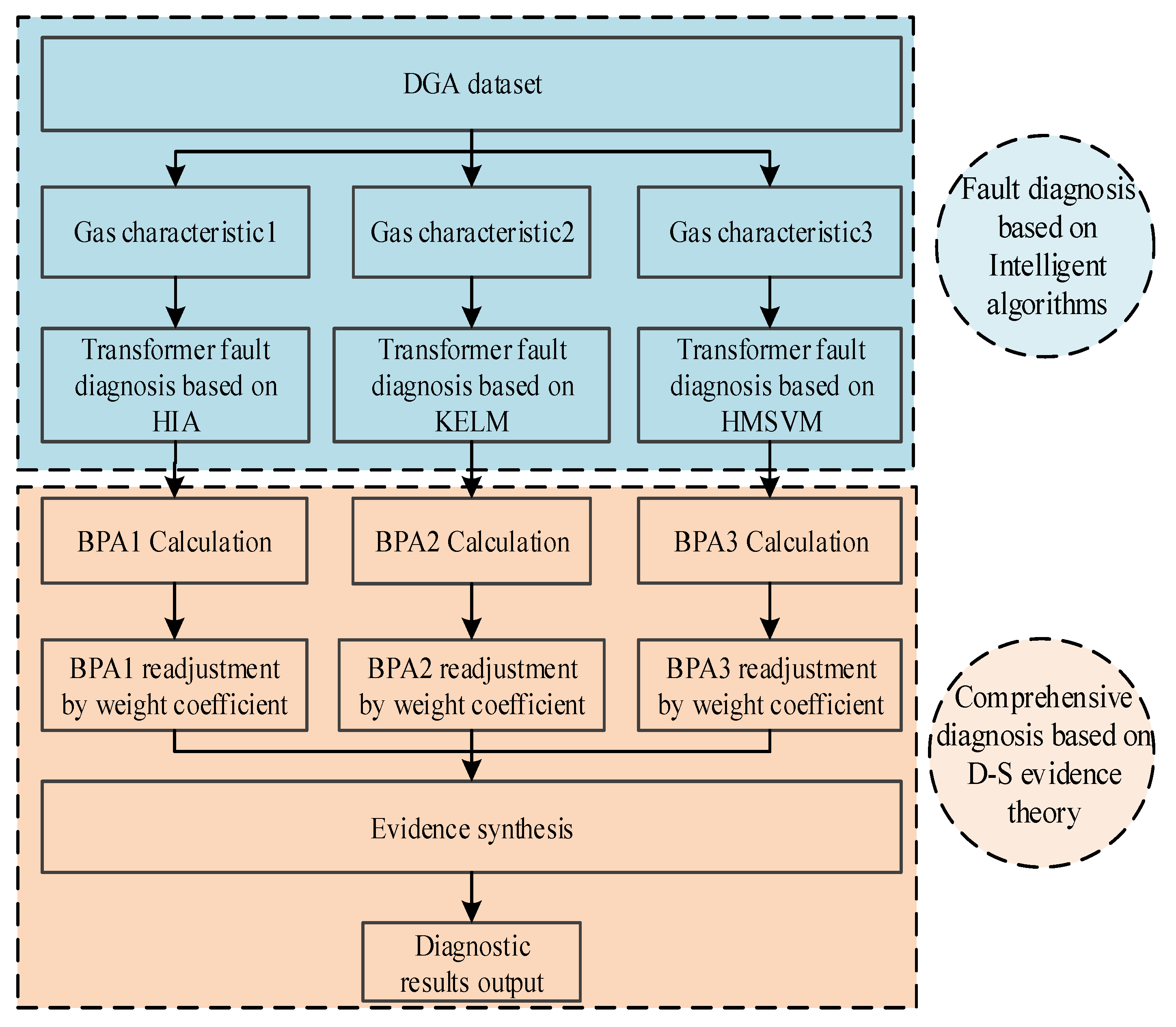
4.2. Transformer Fault Diagnosis Based on Improved D–S Evidence Theory

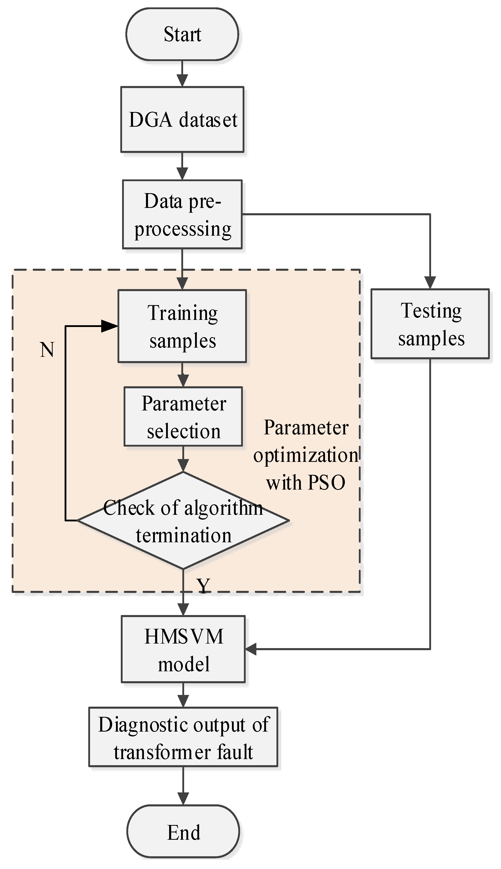
In order to enrich information sources in transformer fault diagnosis and improve the diagnostic efficiency, D–S evidence theory is employed to merge HIA, KELM, and HMSVM together. In this section, a diagnostic fusion model of power transformer fault is constructed based on improved D–S evidence theory. The diagnostic procedure is as follows.

(1)

Three fault diagnosis models are used to test DGA samples and make a preliminary diagnosis. If a unanimous conclusion is obtained, then stop the operation and output the result directly. Otherwise continue the following steps.

(2)

Different BPA of three diagnostic approaches are constructed as follows.

a. HIA

In the recognition framework Θ, the Euclidean distances from A_g to all memory antibodies are calculated. Assuming that the minimum Euclidean distance between A_g and B_i is d_i, if d_i > σ, and then let x_i = 0, otherwise x_i = 1/d_i, where σ is the affinity threshold, i = 1, 2, …, 6. In HIA [40], the BPA of A_g can be described as follows:

$$m_1(B_i)=\frac{x_i}{{\displaystyle \sum _{i=1}^6{x}_j}},i=1,2,\dots ,6$$

(26)

b. KELM

There are 6 kinds of transformer fault states in this paper, that is, the number of recognition types of KELM is 6. If f_i(x) is used to represent the output function for the ith state of transformer faults, then the output function f(x) of KELM is expressed as [41]:

$$f(x)=(f_1(x),f_2(x),\cdots ,f_6(x))$$

(27)

The numerical output of KELM is transformed into probabilistic output.

$$f_i^{\text{'}}(x)=\frac{1}{1+\exp (-f_i(x))},i=1,2,\cdots ,6$$

(28)

For Sample x, the BPA of KELM is defined as:

$$m_2(B_i)=\frac{f_i^{\text{'}}(x)}{{\displaystyle \sum _{i=1}^6{f}_i^{\text{'}}(x)}},i=1,2,\cdots ,6$$

(29)

c. HMSVM

m₃(B_i) denotes the BPA of HMSVM that a group of DGA samples belong to fault A_i.

$$m_3(B_i)=\frac{P(A_i)}{{\displaystyle \sum _{i=1}^{6}P(A_i)}},i=1,2,\dots ,6$$

(30)

where P(A_i) can be calculated by Formula (14).

The above three groups of BPAs are satisfied:

$$\{\begin{array}{c}{\displaystyle \sum _{i=1}^{6}m(B_i)=1}\\ m(\varnothing )=0\end{array}$$

(31)

(3)

The weight coefficient is used to adjust the BPA.

(4)

The synthesized BPA is discriminated according to the following rules.

Let A₁ and A₂ belong to U, satisfying

$$\begin{array}{l}m(A_1)=\max \{m(A_i),A_i\subset \Theta \}\\ m(A_2)=\max \{m(A_i),A_i\subset \Theta \mathrm{and} A_i\ne A_1\}\end{array}$$

(32)

$$\{\begin{array}{c}m(A_1)-m(A_2)>{\epsilon }_1\\ m(\Theta )<{\epsilon }_2\\ m(A_1)>m(\Theta )\end{array}$$

(33)

where A₁ is the judgment result. Further, ε₁ andε₂ are preset thresholds, which are set to be 0.2 after repeated comparison.

The fault diagnosis model based on improved evidence theory is shown in Figure 10.

4.3. Case Analysis and Discussion

In this section, 5 sets of DGA samples are collected from Hebei north electric power company, with actual fault labels attached, shown in

Table 8. Case analysis of transformer fault diagnosis.

Actual Fault	Gas Contents (μL/L)
	H2	CH2	C2H6	C2H4	C2H2
Normal (N)	80	10	4	1.5	0
Overheat caused by screw loose of iron core at 546 °C (T12)	166.6	28.31	6.72	12.4	0.3
Medium and low temperature overheat caused by multipoint earthing of iron core (T12)	89	50	12	140	0
High temperature overheat caused by short circuit between laminated cores (T3)	21	124	5	183	45
High energy discharge caused by discharge between metal rings of fixed iron core (D2)	68.7	9.1	34.88	11.38	1.71

.

The DGA samples are processed and input into the transformer fault diagnosis model based on HMSVM. The output membership values of five groups of samples are obtained, as shown in

Table 9. The memberships of given 5 samples.

Sample Number	Memberships
	N	T12	T3	D1	D2	PD
1	0.8145	0.1688	0.1202	0.2079	0.1007	0.1058
2	0.1836	0.9776	0.0619	0.1085	0.2281	0.1894
3	0.2259	0.5208	0.5429	0.1874	0.2464	0.1507
4	0.2081	0.1898	0.6094	0.2153	0.1964	0.1899
5	0.1804	0.1078	0.2026	0.2128	0.7154	0.1137

. The value appears in bold in Table 9 means the highest membership of each sample.

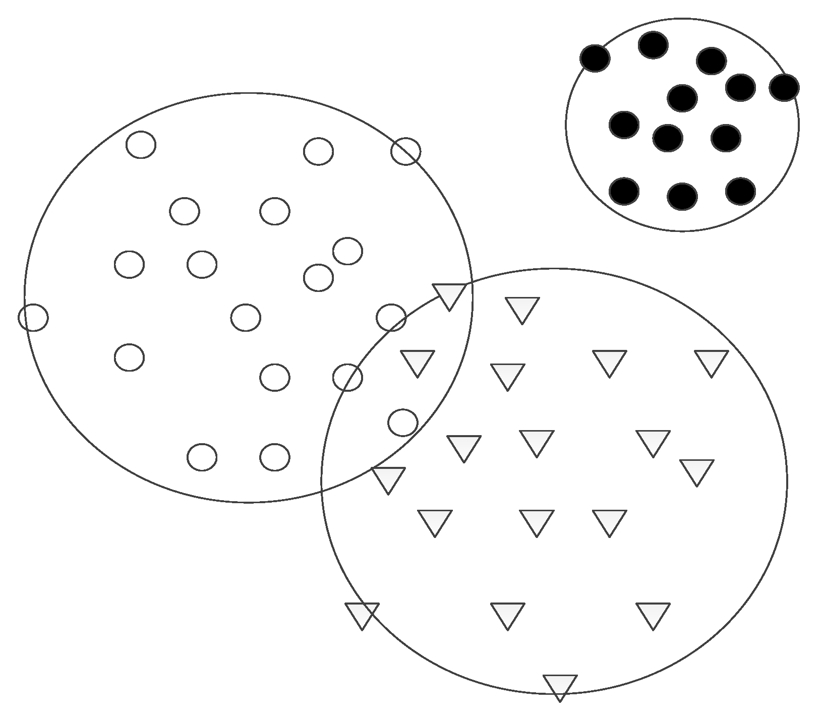
According to the diagnostic principle of HMSVM, if the sample is located inside the hypersphere, the value of membership is greater, otherwise, the value of membership is smaller. Table 9 shows that except for Sample 3, the maximum membership of DGA samples is much greater than that of other fault states. This is because the four samples belong to only one state hypersphere, so the diagnosis conclusion is clear, and the membership value is usually greater than 0.5. For T₁₂ and T₃, the membership values of Sample 3 are greater than 0.5, and close to each other. This is because the sample is located in the overlapping area of hyperspheres, which is prone to misjudgment. According to HMSVM diagnostic criteria, the diagnosis conclusion of this sample is T₃, which is not consistent with the actual fault.

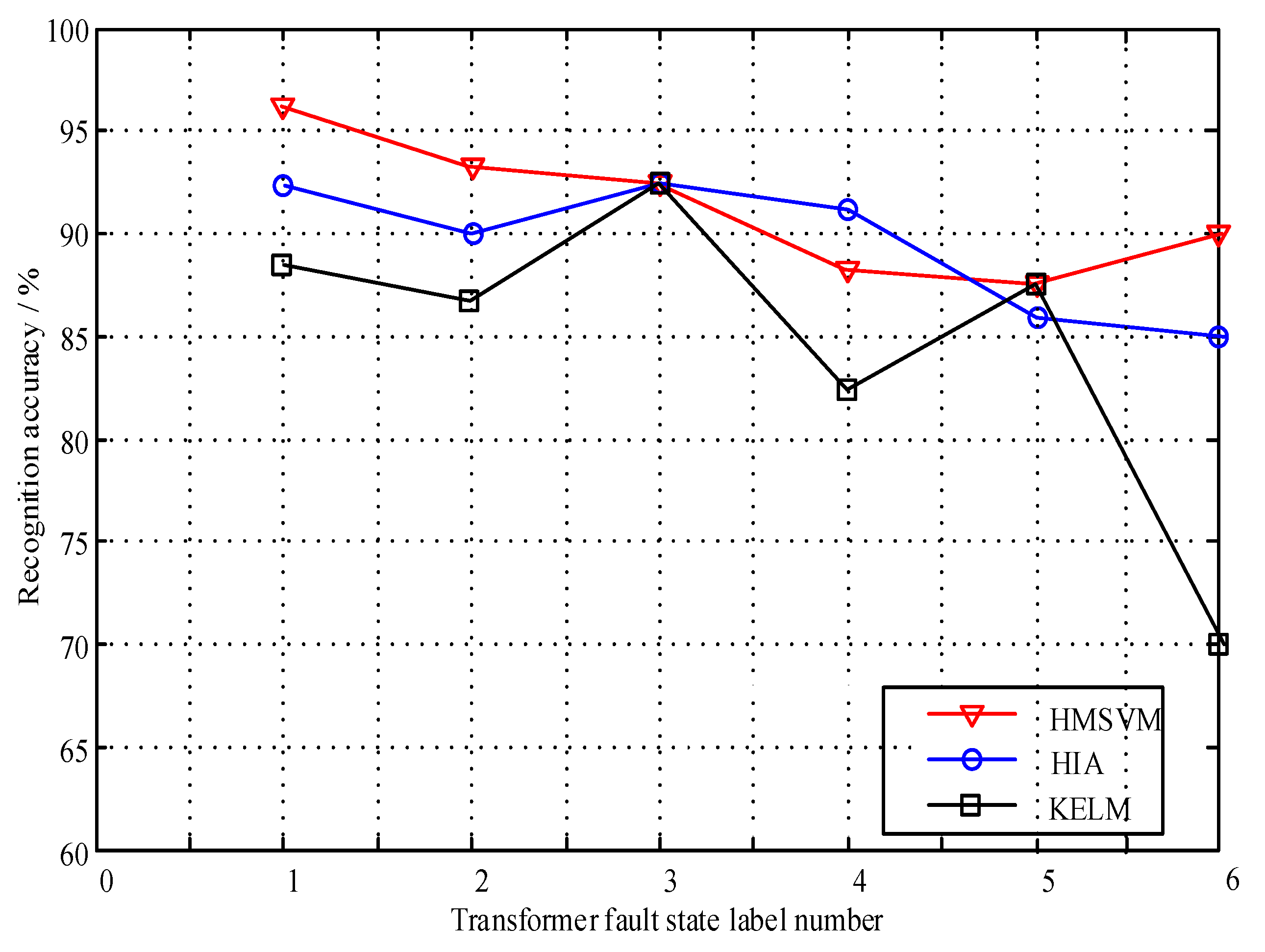
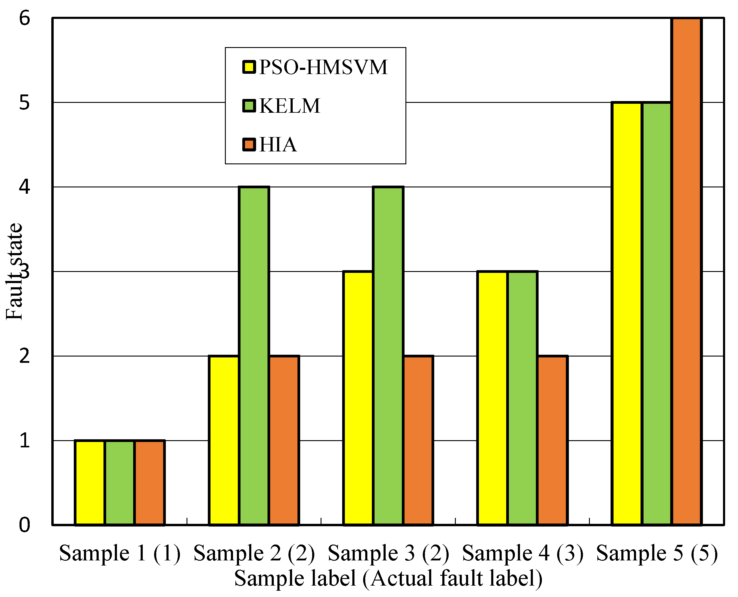
HIA and KELM are employed to analyze above typical samples. The diagnostic results using three intelligent algorithms are shown in Figure 11.

As can be seen from Figure 11, for the five sets of fault samples, the diagnostic results obtained by three intelligent algorithms are quite different. Among them, the HMSVM method has the best diagnostic effect, and only Sample 3 is not recognized correctly. The reason is this sample is located in the overlapping area of hyperspheres, which results in misjudgment. The KELM method has some problems in the diagnosis of Sample 2 and Sample 3, which shows that it is easy to misjudge the overheating fault. The HI method has misjudged Sample 4 and Sample 5, which indicates that this method is not effective for the distinction between high energy discharge and high temperature superheating faults. According to above analysis, except for normal samples, three intelligent methods have great difference in the diagnosis effect of transformer faults. For Sample 3, the diagnostic conclusions given by the three intelligent methods are completely different. Therefore, this paper chooses Sample 3 as the high conflict data for detailed analysis. Afterwards, the evidence theory fusion method is used for comprehensive diagnosis.

In this section, the proposed fusion algorithm is utilized to analyze the high-conflict DGA sample. First of all, the characteristics of the sample are extracted. Then, three different intelligent approaches are employed for preliminary diagnosis. According to the BPA construction method of three different algorithms, the BPA to each fault state is obtained shown in

Table 10. Basic confidence distribution table of primary diagnosis.

Evidences	m(N)	m(T12)	m(T3)	m(D1)	m(D2)	m(PD)
E1	0.0100	0.0172	0.9111	0.0372	0.0038	0.0208
E2	0.0221	0.9679	0	0.0109	0	0
E3	0.0275	0.0302	0.9070	0.0120	0.0086	0.0146

. In the table, E₁, E₂, E₃ represent the evidence of KELM, HIA, and HMSVM respectively, and m denotes the basic probability assignment.

Table 10 shows that the reliability to T₃ is the highest for KELM and HMSVM, and the reliability to T₁₂ is the highest for HIA. The conflictive degree of evidences is calculated, defined as k. k₁₂ denotes the conflictive degree between KELM and HIA. k₁₃ means the conflictive degree between KELM and HMSVM. Lastly, k₂₃ denotes the conflictive degree between HMSVM and HIA. After multiple calculations, the values of k₁₂, k₁₃, k₂₃ are obtained, which are 0.9827, 0.1721, and 0.9700. This indicates that the conflictive degree between HIA and each other evidence is higher.

In order to solve the problem of high conflict between evidences, the weight coefficient is introduced for BPA readjustment. With the degree of conflict k₁₂, k₁₃, k₂₃, the weight coefficient w_i can be obtained by Formulas (20)–(23) as w_i = (0.3845, 0.2335, 0.3819). Due to the serious conflict between E₂ and the other evidence, HIA has smaller weight coefficient. Different weight coefficient values can distinguish the importance degree of each evidence. The uncertainty m(Θ) is introduced in the process of BPA adjustment. The adjusted BPA based on weight coefficients is obtained in

Table 11. Adjusted basic probability assignment (BPA) based on weight coefficients.

Evidence	m(N)	m(T12)	m(T3)	m(D1)	m(D2)	m(PD)	m(Θ)
E123	0.0195	0. 6966	0. 2241	0.0214	0.0047	0.0136	0.0201

.

With the BPA in Table 11, the diagnostic decision can be made by formula (24) and (25). After calculation, m(T₁₂) and m(T₃) are the first and second maximum of basic probability assignment. The difference between these two values is 0.466, which is greater than ε₁(0.2). In addition, the value of uncertainty m(Θ) is 0.0201, which is much less than ε₂(0.2). Above all, the final diagnostic result is T₁₂, which is the same as the actual state.

Using above 253 testing DGA samples, the diagnostic results based on different algorithms are shown in

Table 12. Results comparison.

Algorithms	Diagnostic Accuracy/%
	N	T12	T3	D1	D2	PD	Total
KELM	88.5	86.7	92.4	82.4	87.5	90.0	87.0
HIA	92.3	90.0	92.4	91.2	85.9	85.0	89.7
HMSVM	96.2	93.3	92.4	88.2	87.5	70.0	90.9
IDET	100	96.7	93.7	94.1	92.1	90.0	94.1

.

It can be seen from Table 12 that, due to the superior performance in processing nonhomogeneous and small samples, the total diagnostic accuracy of HMSVM reaches 90.9%, which is better than KELM and HIA. However, for D₁, HIA performs better than HMSVM. In addition, HMSVM gets worse results for PD than both HIA and KELM. It indicates that three intelligent algorithms have diverse performances for different transformer fault states. For each transformer fault state, the diagnostic accuracy of the fusion method based on improved D–S evidence theory is no less than 90.0%. In total, the proposed fusion method has the highest diagnostic accuracy, which is obviously better than the other three single approaches. It shows that IDET can fuse the advantages of each single algorithm together and recognize transformer fault states effectively.

5. Conclusions

Fault diagnosis plays an important role in the safe operation of power transformers. In this study, a novel transformer fault diagnosis approach based on HMSVM was proposed and PSO was applied to parameter optimization. IDET was also introduced to fuse three different diagnostic algorithms together, including HMSVM, HIA, and KELM. The diagnostic results are as follows.

HMSVM uses a hypersphere for pattern recognition, instead of hyperplanes in SVM. It can divide the sample space into different parts with different status and process nonhomogeneous and small samples effectively. Compared with HIA and KELM, HMSVM can get higher accuracy in transformer faults recognition.

The weight coefficient is introduced into DET to solve the problem of high conflict between evidences. It can improve the reliability of evidence fusion.

Transformer fault diagnosis based on IDET can fuse the advantages of three different intelligent algorithms together. IDET provides an effective way for fusion of uncertain information from multiple data sources. The total diagnostic accuracy reaches 94.1%, which is better than each single method.

Due to the diversities of diagnostic performance with different methods, more intelligent approaches could be applied to transformer fault diagnosis and sent into IDET to fuse their advantages together for further consideration.

References

1. Aizpurua, J.I.; McArthur, S.D.; Stewart, B.G.; Lambert, B.; Cross, J.G.; Catterson, V.M. Adaptive Power Transformer Lifetime Predictions through Machine Learning & Uncertainty Modelling in Nuclear Power Plants. IEEE Trans. Ind. Electron. 2019, 66, 4726–4737. [Google Scholar]
2. Ahmed, A. Improved Consistent Interpretation Approach of Fault Type within Power Transformers Using Dissolved Gas Analysis and Gene Expression Programming. Energies 2019, 12, 730. [Google Scholar] [Green Version]
3. Kari, T.; Gao, W.; Zhao, D.; Zhang, Z.; Mo, W.; Wang, Y.; Luan, L. An integrated method of ANFIS and Dempster–Shafer theory for fault diagnosis of power transformer. IEEE Trans. Dielectr. Electr. Insul. 2018, 25, 360–371. [Google Scholar] [CrossRef]
4. Vapnik, V. Statistical Learning Theory; Wiley: New York, NY, USA, 1998; Volume 3, pp. 401–492. [Google Scholar]
5. Huang, S.; Cai, N.; Pacheco, P.P.; Narrandes, S.; Wang, Y.; Xu, W. Applications of Support Vector Machine (SVM) Learning in Cancer Genomics. Cancer Genomics Proteomics 2018, 15, 41–51. [Google Scholar] [Green Version]
6. Yang, X.; Sun, B.; Zhang, X.; Li, L. A Review of Short-term Wind Speed Prediction Based on Support Vector Machine. J. Northeast Electr. Power Univ. 2017, 37, 1–7. [Google Scholar]
7. Gopakumar, P.; Mallikajuna, B.; Reddy, M.J.B.; Mohanta, D.K. Remote monitoring system for real time detection and classification of transmission line faults in a power grid using PMU measurements. Prot. Control Mod. Power Syst. 2018, 3, 16–20. [Google Scholar] [CrossRef]
8. Vippon, P.K.; Sakshi, A. Particle Swarm Optimization based Support Vector Machine (P-SVM) for the Segmentation and Classification of Plants. IEEE Access 2019, 7, 29374–29385. [Google Scholar]
9. Thirumala, K.; Prasad, M.S.; Jain, T.; Umarikar, A.C. Tunable-Q Wavelet Transform and Dual Multiclass SVM for Online Automatic Detection of Power Quality Disturbances. IEEE Trans. Smart Grid 2018, 9, 3018–3028. [Google Scholar] [CrossRef]
10. Schölkopf, B.; Platt, J.C.; Shawe-Taylor, J.; Smola, A.J.; Williamson, R.C. Estimating the support of a high-dimension distribution. Neural Comput. 2001, 7, 1443–1471. [Google Scholar] [CrossRef]
11. Zhang, X.F.; Shen, L.S. A new hypersphere support vector machine algorithm. J. Electron. 2006, 23, 614–617. [Google Scholar] [CrossRef]
12. Wu, Z.; Huang, N.E. Ensemble empirical mode decomposition: A noise-assisted data analysis method. Adv. Adapt. Data Anal. 2019, 1, 1–41. [Google Scholar] [CrossRef]
13. Ai, Q.; Wang, A.; Wang, Y.; Sun, H. Improvements on twin-hypersphere support vector machine using local density information. Prog. Artif. Intell. 2018, 7, 167–175. [Google Scholar] [CrossRef]
14. Zhu, M.L.; Liu, X.D.; Chen, S.F. Solving the Problem of Multi-class Pattern Recognition with Sphere-structured Support Vector Machines. Nat. Sci. 2003, 39, 153–158. [Google Scholar]
15. Sun, A.X.; Huang, S.L.; Li, M.H.; Zhang, J. A new hypersphere multi-class support vector machine applied in text classification. In Proceedings of the IEEE International Conference on Communication Software & Networks, Xi’an, China, 27–29 May 2011; pp. 478–481. [Google Scholar]
16. Shang, H.K.; Li, F.; Wu, Y.J. Partial Discharge Fault Diagnosis Based on Multi-Scale Dispersion Entropy and a Hypersphere Multiclass Support Vector Machine. Entropy 2019, 21, 81. [Google Scholar] [CrossRef]
17. Wang, D.; Liu, Y.; Wu, Z.; Fu, H.; Shi, Y.; Guo, H. Scenario Analysis of Natural Gas Consumption in China Based on Wavelet Neural Network Optimized by Particle Swarm Optimization Algorithm. Energies 2018, 11, 825. [Google Scholar] [CrossRef]
18. Jain, N.K.; Nangia, U.; Jain, J. A Review of Particle Swarm Optimization. J. Inst. Eng. 2018, 99, 407–411. [Google Scholar] [CrossRef]
19. Azil, I.H.; Wee, Z.L.; Li, X.T. Identification of transformer fault based on dissolved gas analysis using hybrid support vector machine-modified evolutionary particle swarm optimization. PLoS ONE 2018, 13, e0191366. [Google Scholar]
20. Sentz, K. Combination of Evidence in Dempster–Shafer Theory. Contemp. Pac. 2002, 11, 416–426. [Google Scholar]
21. Xiao, F.; Qin, B.W. A Weighted Combination Method for Conflicting Evidence in Multi-Sensor Data Fusion. Sensors 2018, 18, 1487. [Google Scholar] [CrossRef]
22. Chatterjee, M.; Namin, A.S. Detecting Web Spams Using Evidence Theory. In Proceedings of the IEEE Computer Software & Applications Conference, Tokyo, Japan, 23–27 July 2018; pp. 695–700. [Google Scholar]
23. Gui, L.; Yang, X.; Cremers, A.B.; Chen, Y. Dempster–Shafer Evidence Theory-Based CV Model for Renal Lesion Segmentation of Medical Ultrasound Images. J. Med. Imaging Health Inform. 2017, 7, 595–606. [Google Scholar] [CrossRef]
24. Hui, K.H.; Lim, M.H.; Leong, M.S.; Al-Obaidi, S.M. Dempster–Shafer evidence theory for multi-bearing faults diagnosis. Eng. Appl. Artif. Intell. 2017, 57, 160–170. [Google Scholar] [CrossRef]
25. Jiang, W.; Cao, Y.; Yang, L.; He, Z. A Time-Space Domain Information Fusion Method for Specific Emitter Identification Based on Dempster–Shafer Evidence Theory. Sensors 2017, 17, 1972. [Google Scholar] [CrossRef] [PubMed]
26. Denoeux, T.; Li, S.; Sriboonchitta, S. Evaluating and Comparing Soft Partitions: An Approach Based on Dempster–Shafer Theory. IEEE Trans. Fuzzy Syst. 2018, 26, 1231–1244. [Google Scholar] [CrossRef]
27. Ramachandran, B.; Srivastava, S.K.; Edrington, C.S.; Cartes, D.A. An Intelligent Auction Scheme for Smart Grid Market Using a Hybrid Immune Algorithm. IEEE Trans. Ind. Electron. 2011, 58, 4603–4612. [Google Scholar] [CrossRef]
28. Rabbani, M.; Panahi, H. An Efficient Hybrid Artificial Immune Algorithm for Clustering. In Proceedings of the 2008 Eighth International Conference on Hybrid Intelligent Systems, Barcelona, Spain, 10–12 September 2008; pp. 374–379. [Google Scholar]
29. Pandey, P.; Patel, V.; George, N.V.; Mallajosyula, S.S. KELM-CPPpred: Kernel Extreme Learning Machine Based Prediction Model for Cell-Penetrating Peptides. J. Proteome Res. 2018, 17, 3214–3222. [Google Scholar] [CrossRef] [PubMed]
30. Xiao, L.Y.; Shao, W.; Ding, X.; Wang, B.Z. Dynamic Adjustment Kernel Extreme Learning Machine for Microwave Component Design. IEEE Trans. Microw. Theory Tech. 2018, 66, 4452–4461. [Google Scholar] [CrossRef]
31. Suma, T.; Murugesan, R. Artificial Immune Algorithm for Subtask Industrial Robot Scheduling in Cloud Manufacturing. J. Phys. Conf. Ser. 2018, 1000, 1–8. [Google Scholar] [CrossRef]
32. Gupta, S.; Karanath, A.; Mahrifa, K.; Dileep, A.D.; Thenkanidiyoor, V. Segment-level probabilistic sequence kernel and segment-level pyramid match kernel based extreme learning machine for classification of varying length patterns of speech. Int. J. Speech Technol. 2019, 22, 231–249. [Google Scholar] [CrossRef]
33. Fang, X.Z.; Zhang, W.; Teng, S.H.; Han, N. Cooperative Intrusion Detection Method Based on δ-HSSVM. Comput. Eng. 2011, 37, 100–101, 104. [Google Scholar]
34. Guo, Y.; Xiao, H. Multiclass multiple kernel learning using hypersphere for pattern recognition. Appl. Intell. 2017, 48, 2746–2754. [Google Scholar] [CrossRef]
35. Nabila, E.; Elmogy, M.; Khalifa, F.; Ghazal, M.; Ghazi, N.; Aboelfetouh, A.; Riad, A.; Sandhu, H.; Schaal, S.; El-Baz, A. Early Diabetic Retinopathy Diagnosis Based on Local Retinal Blood Vessels Analysis in Optical Coherence Tomography Angiography (OCTA) Images. Med. Phys. 2018, 45, 1–17. [Google Scholar]
36. Eberhart, R.C.; Shi, Y.H. Particle swarm optimization: Developments, applications and resources. In Proceedings of the Congress on Evolutionary Computation, Honolulu, HI, USA, 12–17 May 2002; pp. 81–86. [Google Scholar]
37. Zhang, L.W. Fault Diagnosis of Oil-Immersed Transformers Using Self-Organization Antibody Network and Immune Operator. Math. Probl. Eng. 2014, 2, 1–8. [Google Scholar] [CrossRef]
38. Dai, J.; Song, H.; Sheng, G.; Jiang, X. Dissolved gas analysis of insulating oil for power transformer fault diagnosis with deep belief network. IEEE Trans. Dielectr. Electr. Insul. 2017, 24, 2828–2835. [Google Scholar] [CrossRef]
39. Li, S.; Liu, G.; Tang, X.; Lu, J.; Hu, J. An Ensemble Deep Convolutional Neural Network Model with Improved D–S Evidence Fusion for Bearing Fault Diagnosis. Sensors 2017, 17, 1729. [Google Scholar] [CrossRef] [PubMed]
40. Taher, S.A.; Amooshahi, M.K. New approach for optimal UPFC placement using hybrid immune algorithm in electric power systems. Int. J. Electr. Power Energy Syst. 2012, 43, 899–909. [Google Scholar] [CrossRef]
41. Liu, X.; Wang, L.; Huang, G.B.; Zhang, J.; Yin, J. Multiple kernel extreme learning machine. Neurocomputing 2015, 149, 253–264. [Google Scholar] [CrossRef]
Figure 1. Hypersphere support vector machine (HSSVM) schematic diagram.
Energies 12 04017 g001
Figure 2. Hypersphere multiclass support vector machine (HMSVM) classification model.
Energies 12 04017 g002
Figure 3. Boundaries of HMSVM vary with different parameters.
Energies 12 04017 g003
Figure 4. Influence of C on the radius of HMSVM.
Energies 12 04017 g004
Figure 5. Influence of σ on the radius of HMSVM.
Energies 12 04017 g005
Figure 6. Flow chart of particle swarm optimization (PSO)-HMSVM.
Energies 12 04017 g006
Figure 7. Flow chart of transformer fault diagnosis based on PSO-HMSVM.
Energies 12 04017 g007
Figure 8. Fitness curve of parameters in HMSVM.
Energies 12 04017 g008
Figure 9. Diagnosis results of three intelligent algorithms.
Energies 12 04017 g009
Figure 10. The fault diagnosis model of power transformer based on improved evidence theory.
Energies 12 04017 g010
Figure 11. Diagnostic results with different algorithms.
Energies 12 04017 g011