Adaptive Robust Simultaneous Stabilization of Two Dynamic Positioning Vessels Based on a Port-Controlled Hamiltonian (PCH) Model


Abstract

1. Introduction
2. Problem Formulation and Preliminaries
2.1. Some Lemmas
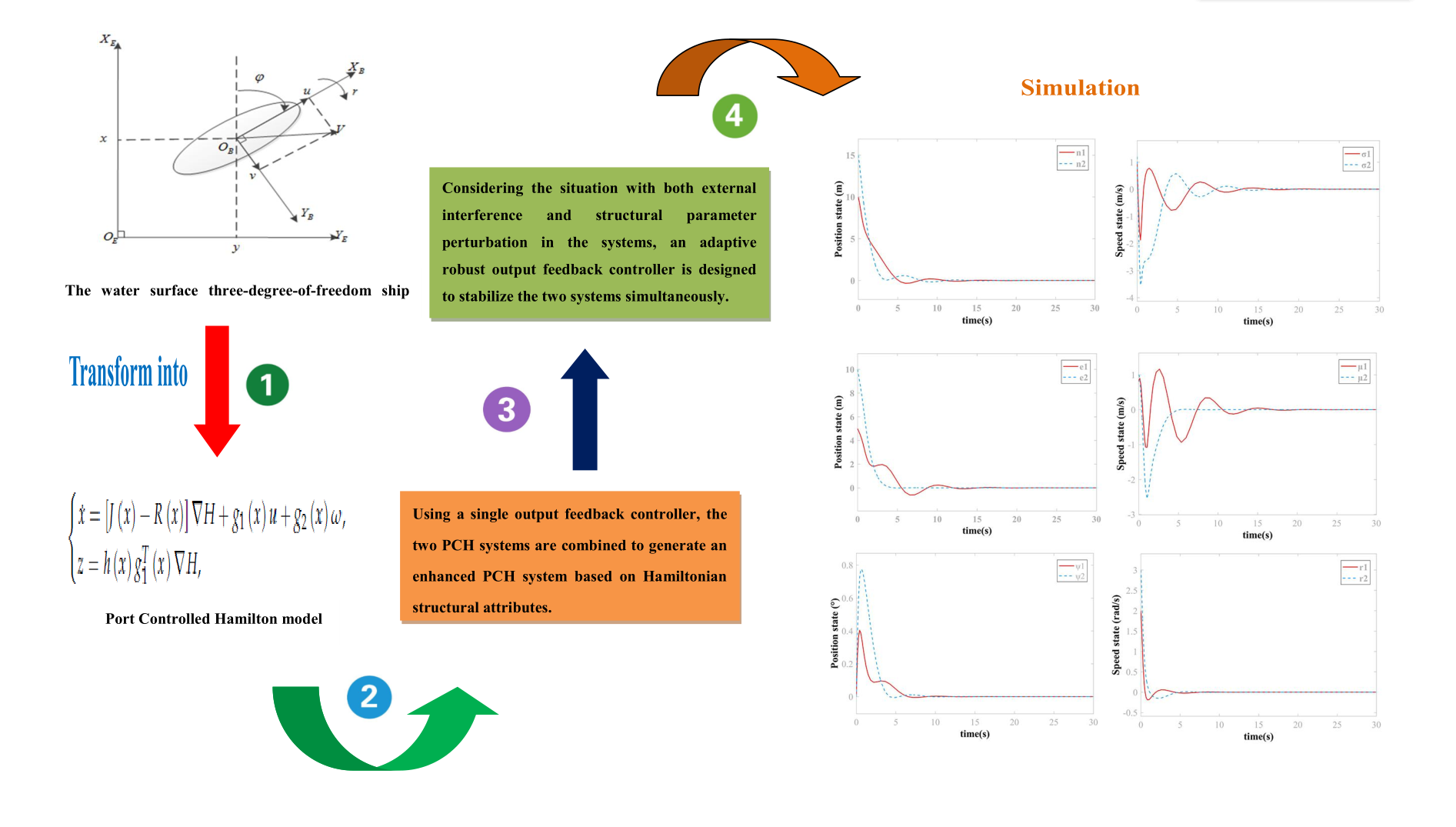
2.2. Dynamic Model of Ship
3. Adaptive Robust Simultaneous Stabilization
3.1. Simultaneous Stabilization
3.2. Adaptive Simultaneous Stabilization
- (i)
- there exists a symmetric matrix such thatwhere ;
- (ii)
- there exists a matrix Φ with appropriate dimension such thatwhere , θ is an unknown constant vector related to and .
3.3. Adaptive Robust Simultaneous Stabilization
- (a)
- (b)
- The gain (from to z ) of the closed-loop system is not greater than the given .
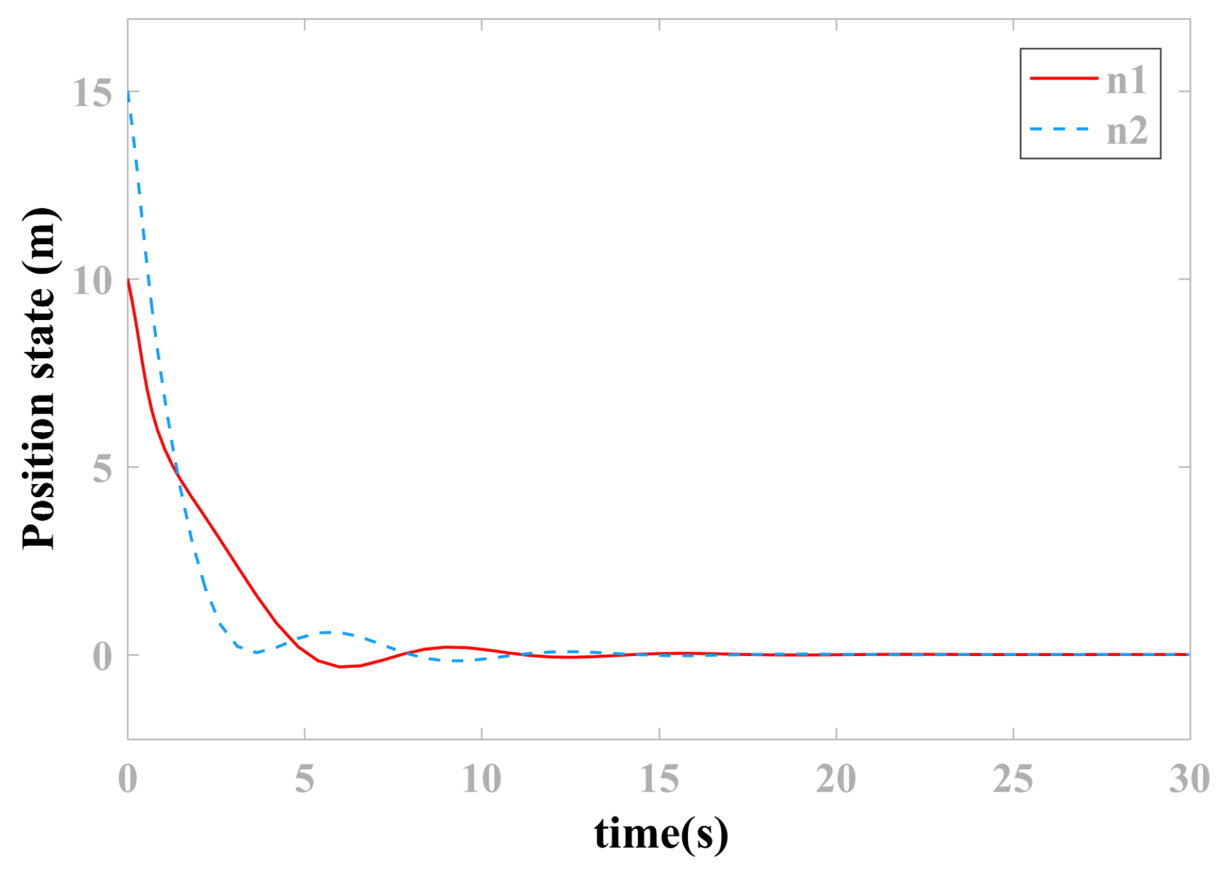
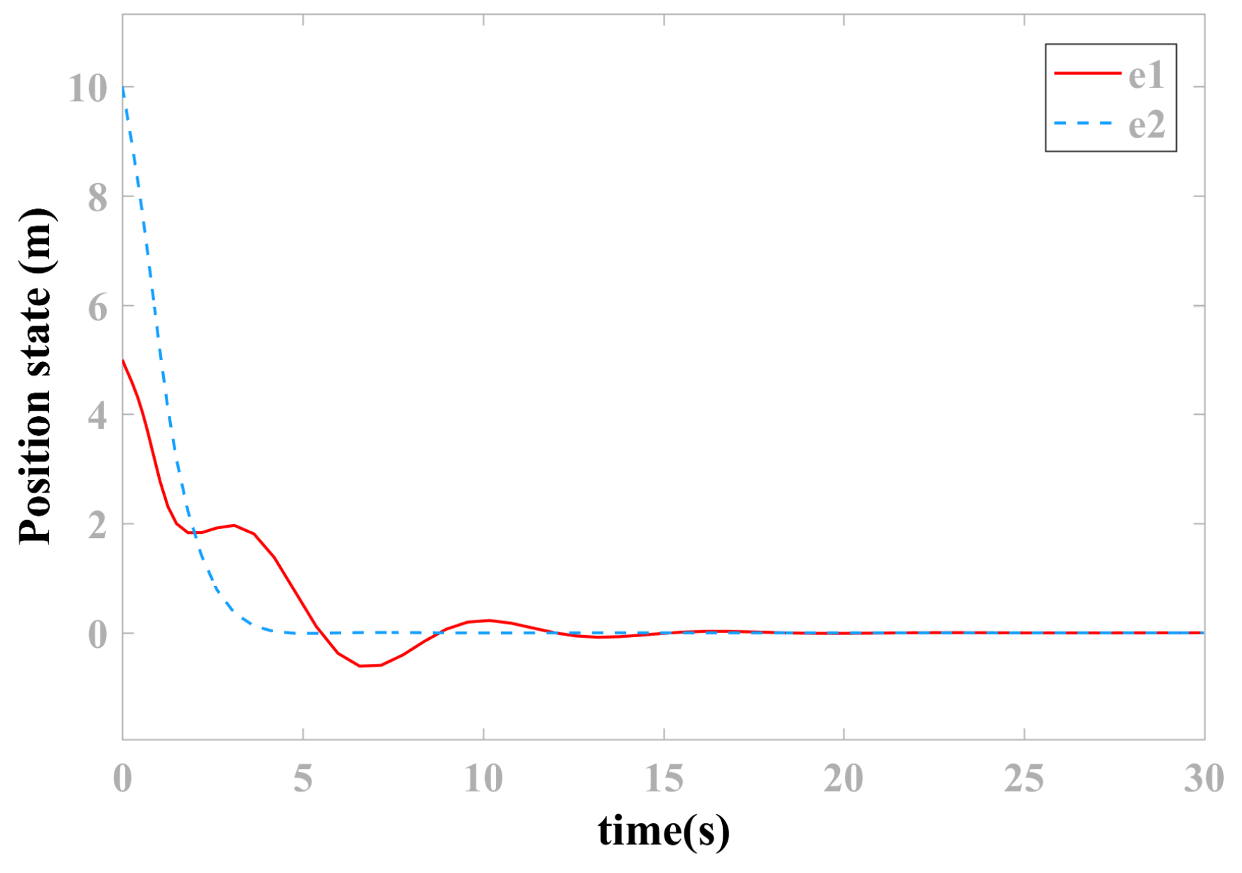
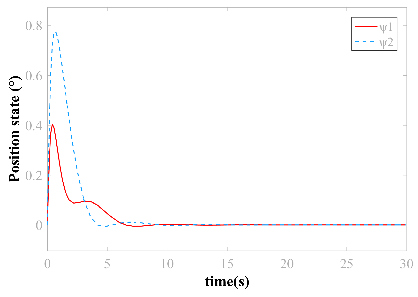
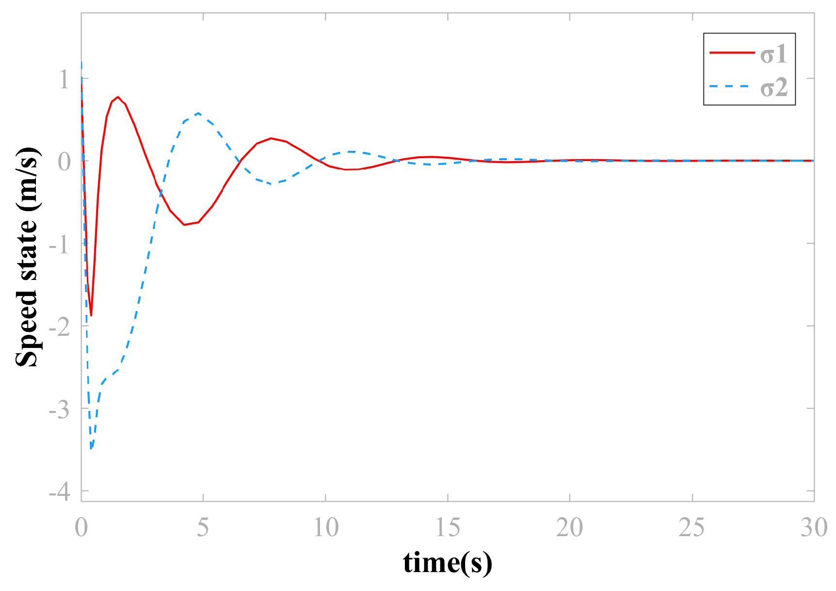
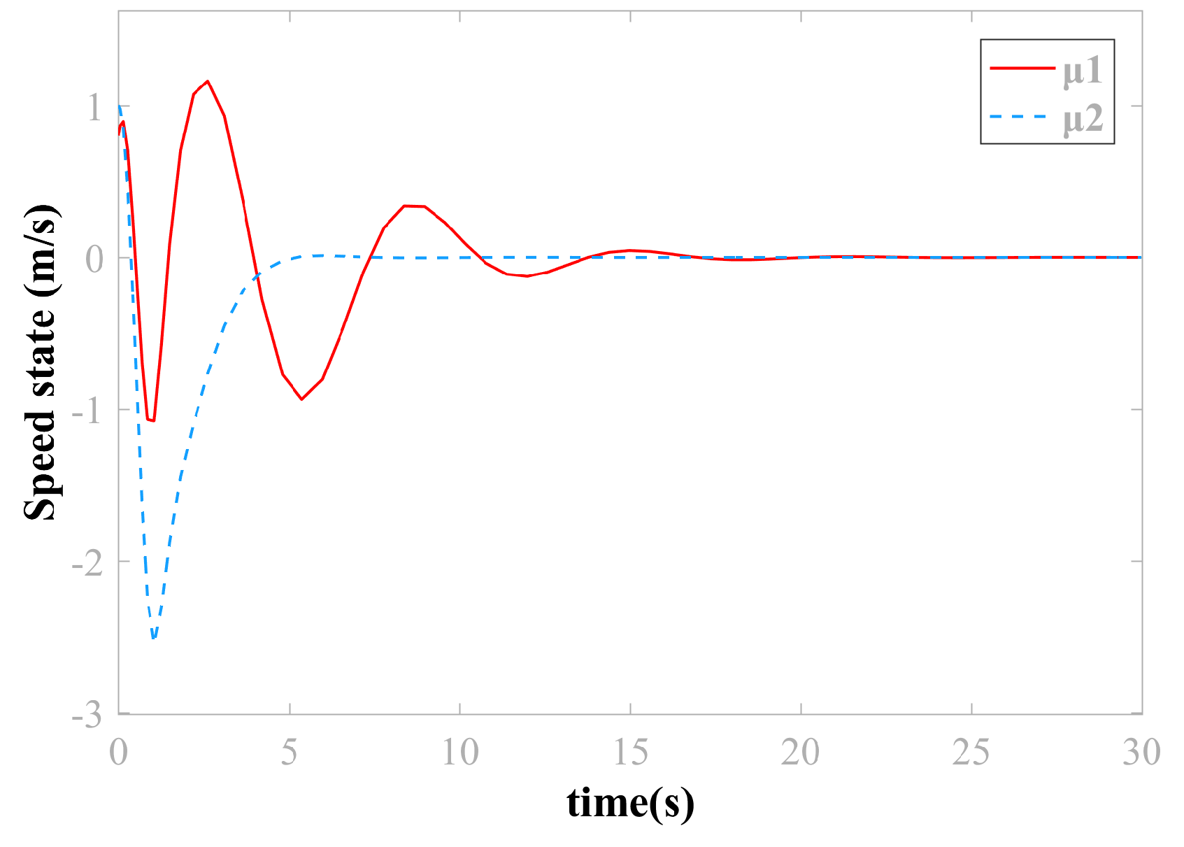
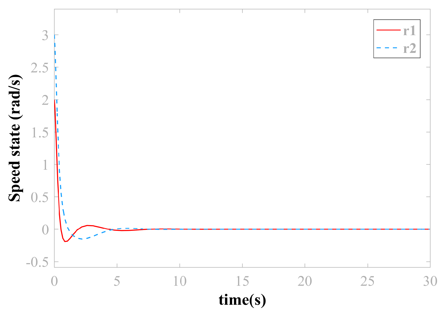
4. Simulation
5. Conclusions
Author Contributions
Funding
Conflicts of Interest
References
- Bian, X.; Fu, M.; Wang, Y. Ship Dynamic Positioning; Science Press: Beijing, China, 2011; pp. 1–13. [Google Scholar]
- Ding, X. Ship Dynamic Positioning Control System; Dalian Maritime University Press: Dalian, China, 2017; pp. 1–30. [Google Scholar]
- Jiao, J.; Wang, G.; Gu, Y.; Sun, X. Coordinated Formation Control of Dynamically Positioned Ships; Electronic Industry Press: Beijing, China, 2017; pp. 1–20. [Google Scholar]
- Wang, B. Robust Adaptive Formation Control for Multiple Dynamic Positioning Vessels. Ph.D. Thesis, Harbin Engineering University, Harbin, China, 2017. [Google Scholar]
- Wang, S. Research on Consistency Theory of Multi-Dynamic Positioning Vessels. Ph.D. Thesis, Harbin Engineering University, Harbin, China, 2014. [Google Scholar]
- Li, Y.; Xu, F.; Xie, G. Overview of the development and application of multi-agent technology. Comput. Eng. Appl. 2018, 54, 13–21. [Google Scholar]
- Xu, G. Research on Unified Multi-Agent System and Formation Control Design. Ph.D. Thesis, Taiyuan University, Taiyuan, China, 2018. [Google Scholar]
- Chen, G. Study on the Stabilization Control of Underactuated Surface Vessels. Ph.D. Thesis, Dalian Maritime University, Dalian, China, 2014. [Google Scholar]
- Kang, Z.; Zou, J.; Fang, L. Design of a motion stabilization controller for a fully driven ship. SHIP BOAT 2018, 29, 51–58. [Google Scholar]
- Muhammad, S.; DoRia-Cerezo, A. Passivity-based control applied to the dynamic positioning of ships. IET Control Theory Appl. 2012, 6, 680–688. [Google Scholar] [CrossRef]
- Tu, F.; Ge, S.; Choo, Y.S.; Hang, C.C. Adaptive Dynamic Positioning Control for Accommodation Vessels with Multiple Constraints. IET Control Theory Appl. 2016, 11, 329–340. [Google Scholar] [CrossRef]
- Mao, J. Simultaneous Stabilization and Simultaneous H∞ Control for Uncertain Nonlinear Systems. Ph.D. Thesis, Zhengzhou University, Zhengzhou, China, 2011. [Google Scholar]
- Cai, X.; Gao, H.; Liu, Y. Simultaneous H∞ Stabilization for a Class of Multi-input Nonlinear Systems. Acta Autom. Sin. 2012, 38, 473–478. [Google Scholar] [CrossRef]
- Wang, Y.; Liu, Y.; Gang, F. Simultaneous stabilization of nonlinear port-controlled Hamiltonian systems via output feedback. J. Shandong Univ. Eng. Sci. 2009, 39, 52–63. [Google Scholar]
- Zhang, J. Simultaneous Stabilization and Control Stydy of Time-delay Systems. Ph.D. Thesis, Inner Mongolia Normal University, Hohhot, China, 2016. [Google Scholar]
- Li, R. Simultaneous Stabilization and Control for Singular Systems with Time-delay. Ph.D. Thesis, Inner Mongolia Normal University, Hohhot, China, 2016. [Google Scholar]
- Liang, Y. Simultaneous Stabilization and Control for Inter-connected Large-scale System with Time-delay. Ph.D. Thesis, Inner Mongolia Normal University, Hohhot, China, 2016. [Google Scholar]
- Wang, Y. Generalized Hamiltonian Control System Theory: Implementation, Control and Application; Science Press: Beijing, China, 2017. [Google Scholar]
- Fossen, T.I. Handbook of Marine Craft Hydrodynamics and Motion Control; John Wiley and Sons Ltd. Press: West Sussex, UK, 2011; pp. 45–58. [Google Scholar]
- Wang, Y.; Gang, F.; Cheng, D. Simultaneous stabilization of a set of nonlinear port-controlled Hamiltonian systems. Automatica 2007, 43, 403–415. [Google Scholar] [CrossRef]
- Yang, R.; Guo, R. Adaptive finite-time robust control of nonlinear delay Hamiltonian systems via Lyapunov-Krasovskii method. Asian J. Control 2018, 20, 1–11. [Google Scholar] [CrossRef]
- Hu, X. Reserch on Nonlinear Control for Dynamic Positioning of Ships. Ph.D. Thesis, Dalian Maritime University, Dalian, China, 2018. [Google Scholar]


© 2019 by the authors. Licensee MDPI, Basel, Switzerland. This article is an open access article distributed under the terms and conditions of the Creative Commons Attribution (CC BY) license (http://creativecommons.org/licenses/by/4.0/).
Share and Cite
Zhou, P.; Yang, R.; Zhang, G.; Han, Y. Adaptive Robust Simultaneous Stabilization of Two Dynamic Positioning Vessels Based on a Port-Controlled Hamiltonian (PCH) Model. Energies 2019, 12, 3936. https://doi.org/10.3390/en12203936
Zhou P, Yang R, Zhang G, Han Y. Adaptive Robust Simultaneous Stabilization of Two Dynamic Positioning Vessels Based on a Port-Controlled Hamiltonian (PCH) Model. Energies. 2019; 12(20):3936. https://doi.org/10.3390/en12203936
Chicago/Turabian StyleZhou, Pei, Renming Yang, Guangyuan Zhang, and Yaozhen Han. 2019. "Adaptive Robust Simultaneous Stabilization of Two Dynamic Positioning Vessels Based on a Port-Controlled Hamiltonian (PCH) Model" Energies 12, no. 20: 3936. https://doi.org/10.3390/en12203936
APA StyleZhou, P., Yang, R., Zhang, G., & Han, Y. (2019). Adaptive Robust Simultaneous Stabilization of Two Dynamic Positioning Vessels Based on a Port-Controlled Hamiltonian (PCH) Model. Energies, 12(20), 3936. https://doi.org/10.3390/en12203936