Adaptive-Gain Second-Order Sliding Mode Direct Power Control for Wind-Turbine-Driven DFIG under Balanced and Unbalanced Grid Voltage

Abstract
1. Introduction
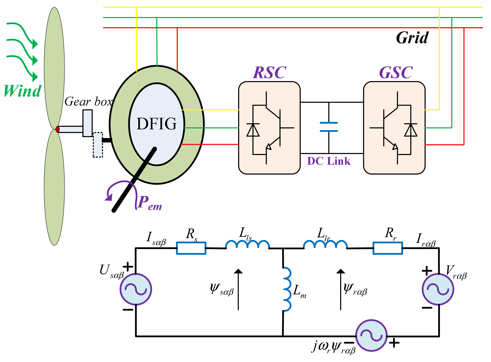
2. Model Analysis
3. Second-Order Sliding Mode Direct Power Controller Design
4. Simulation Results
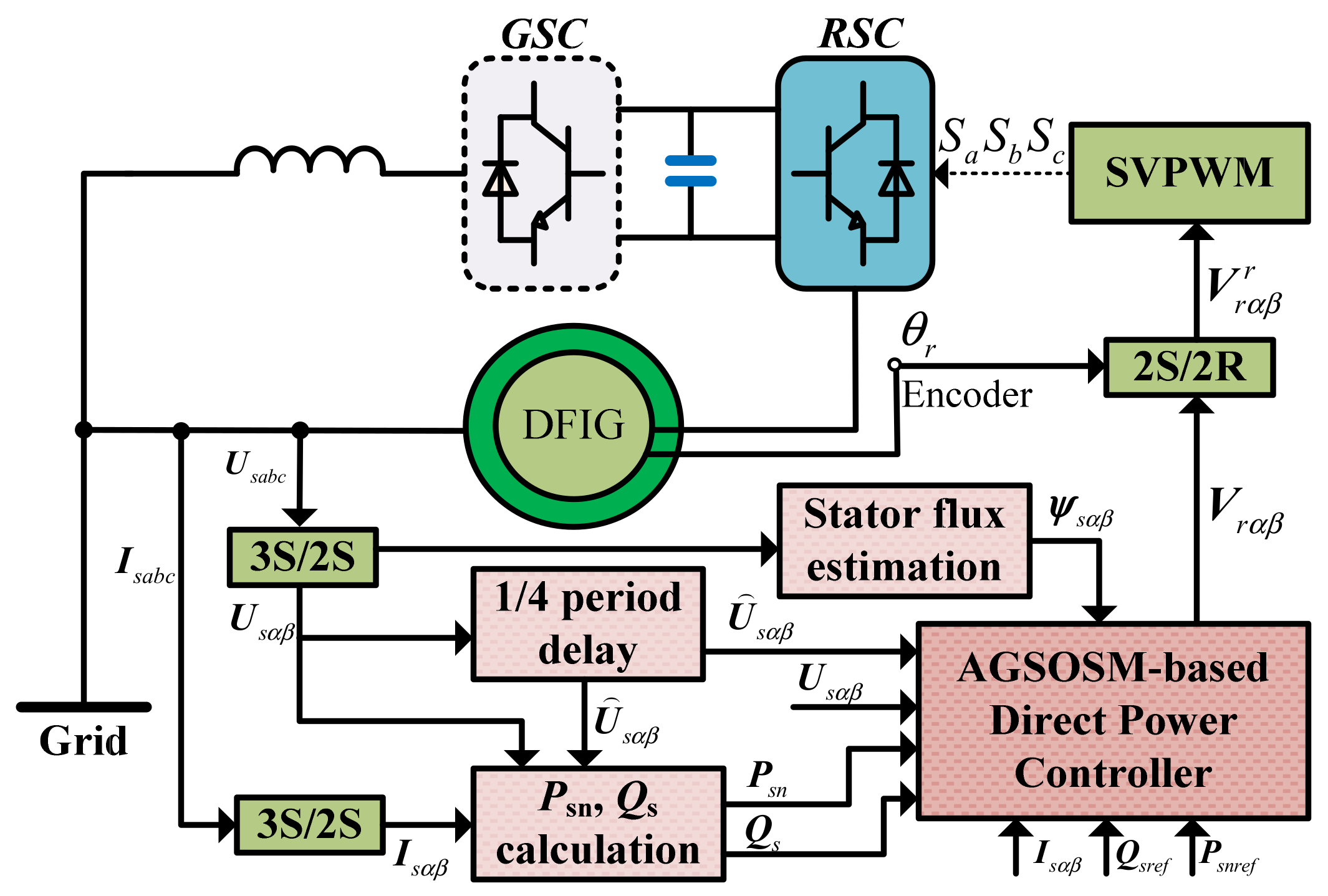
4.1. Control System Overview
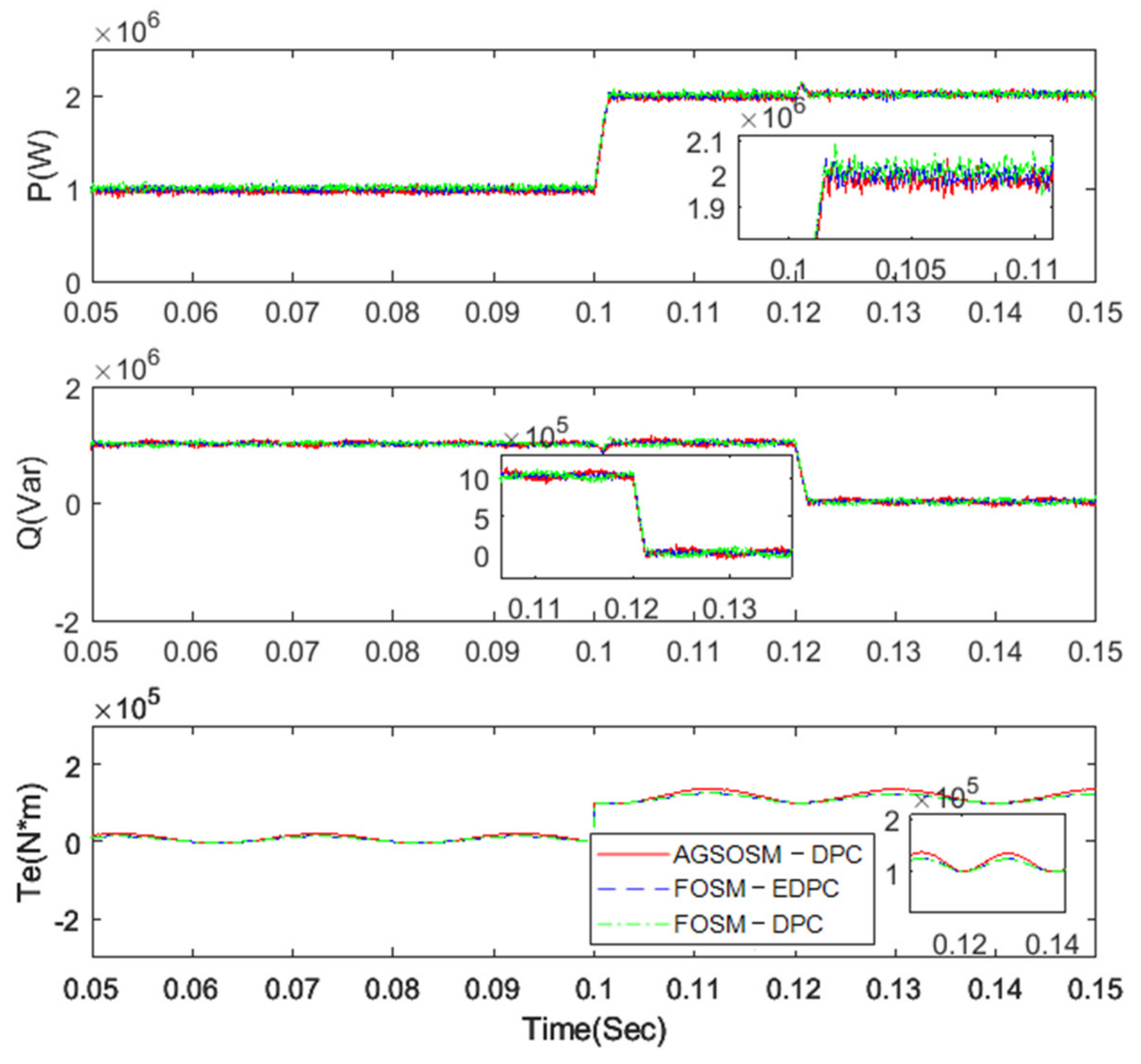
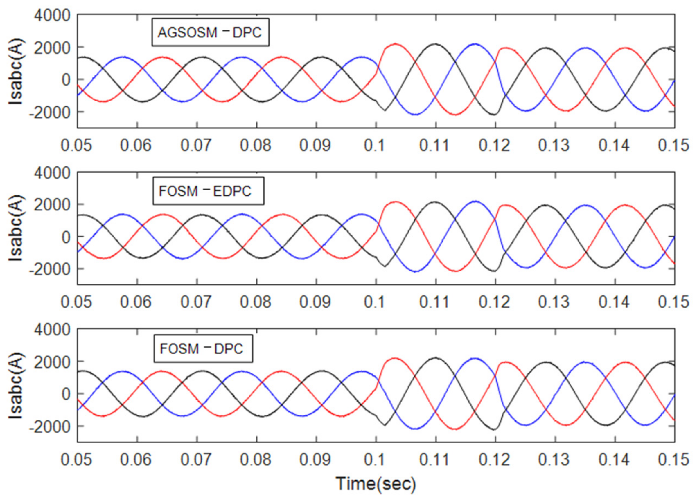
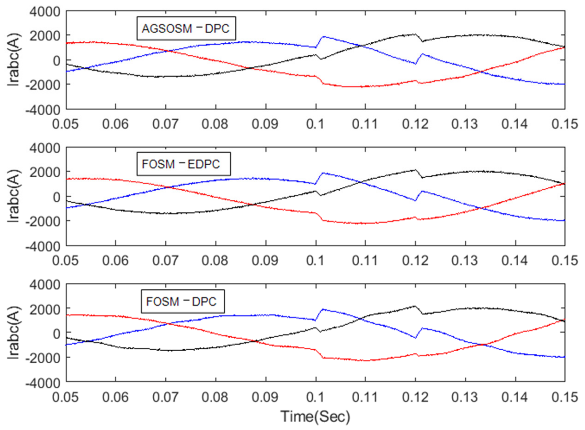
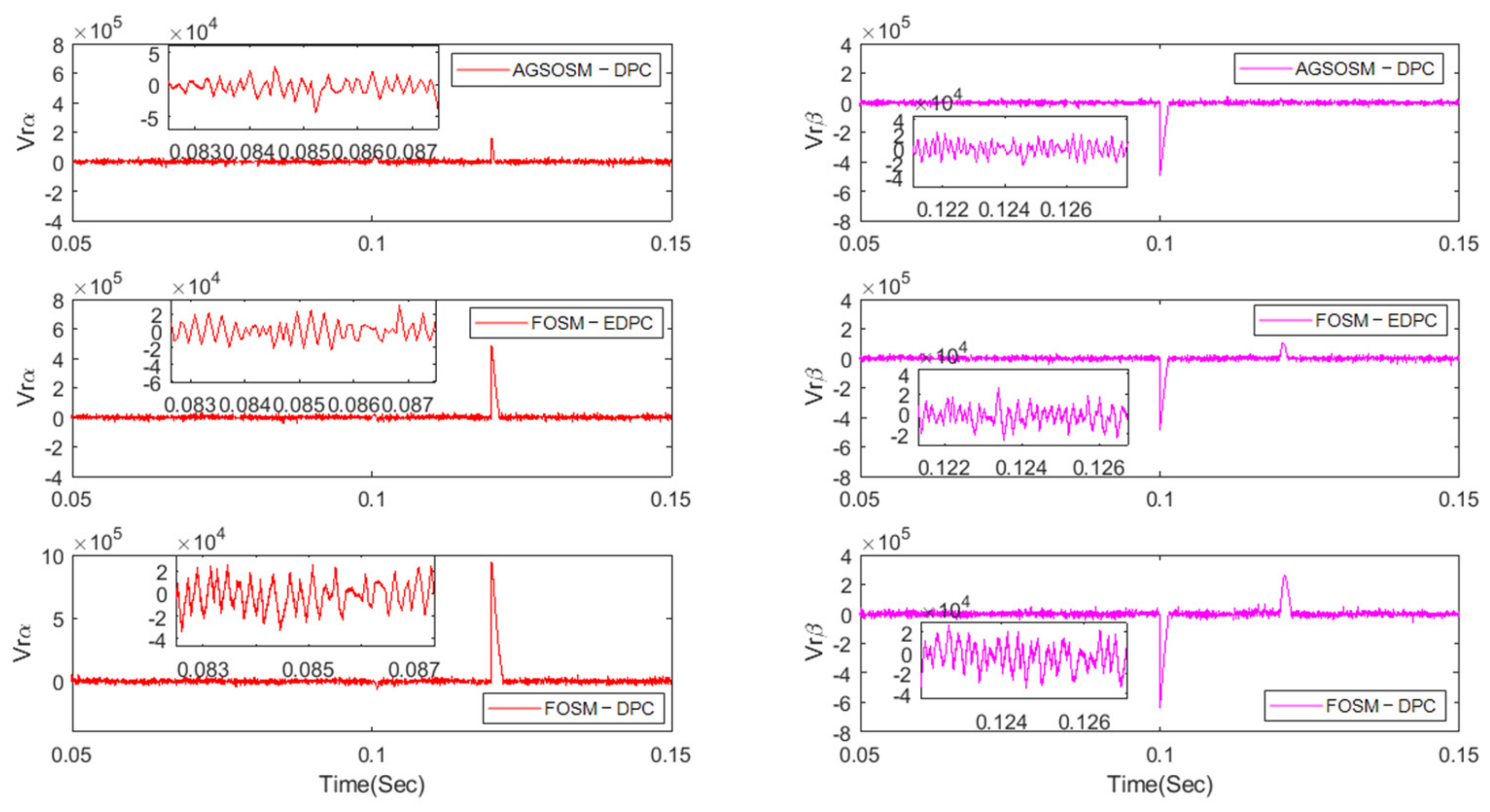
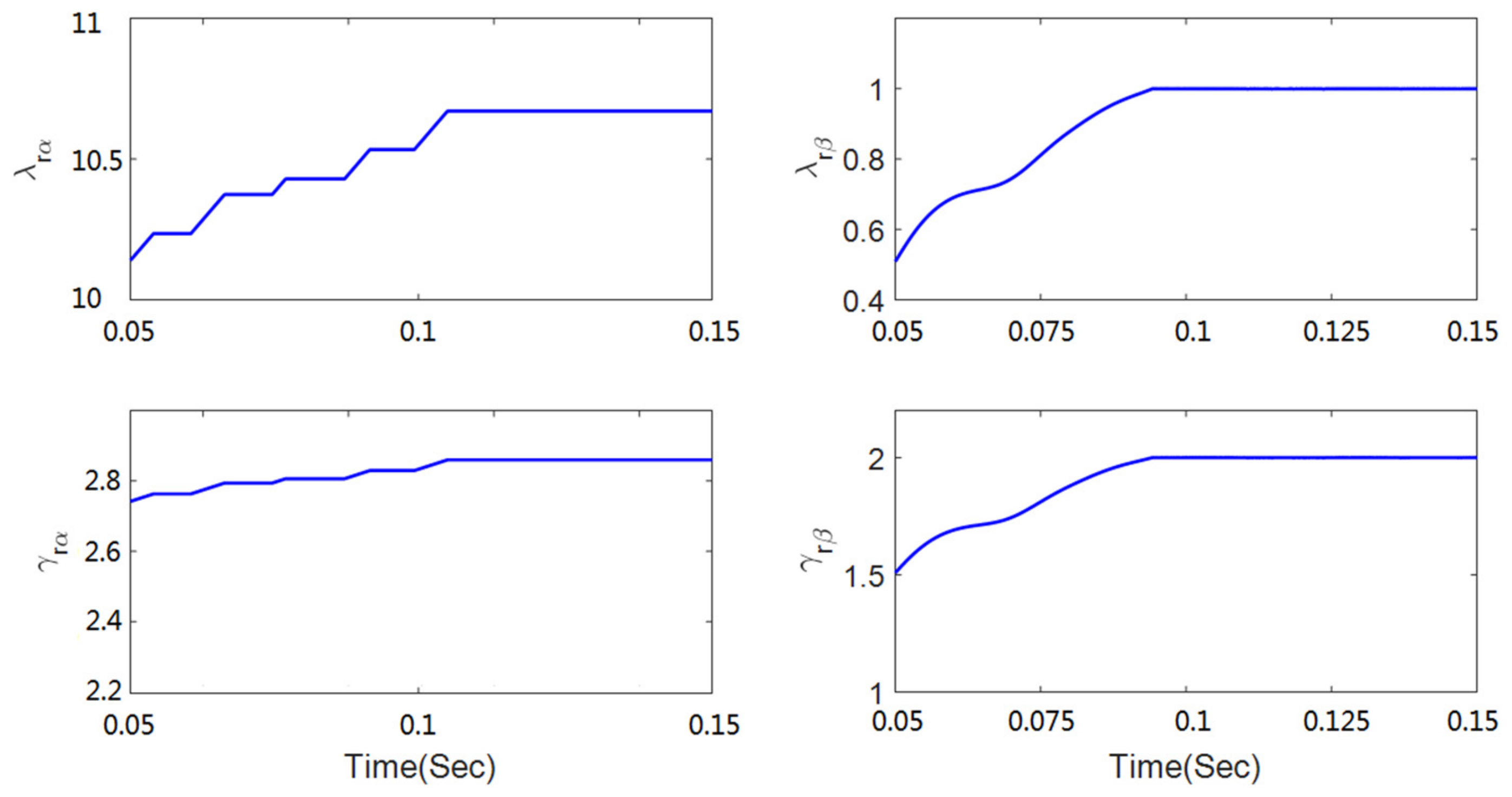
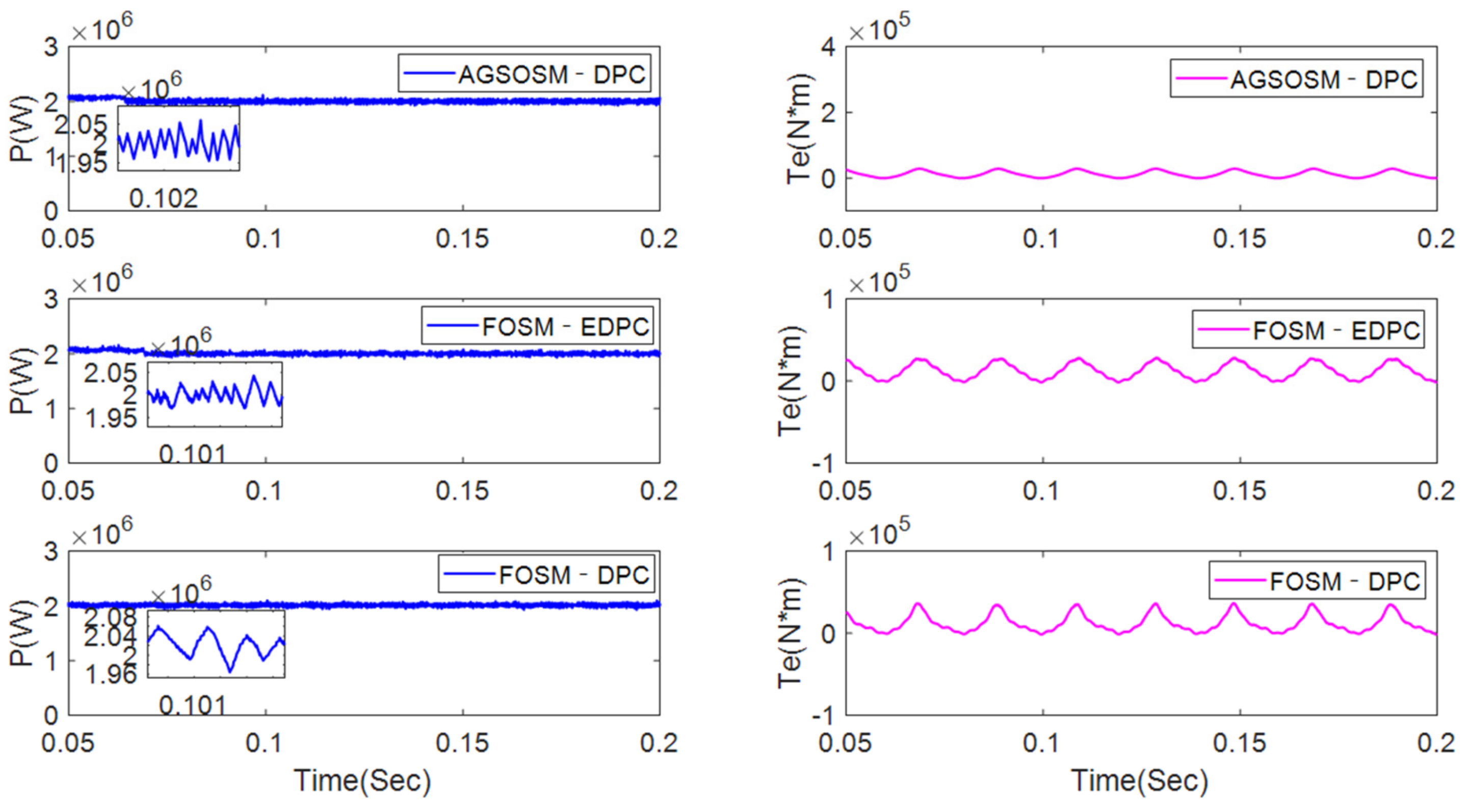
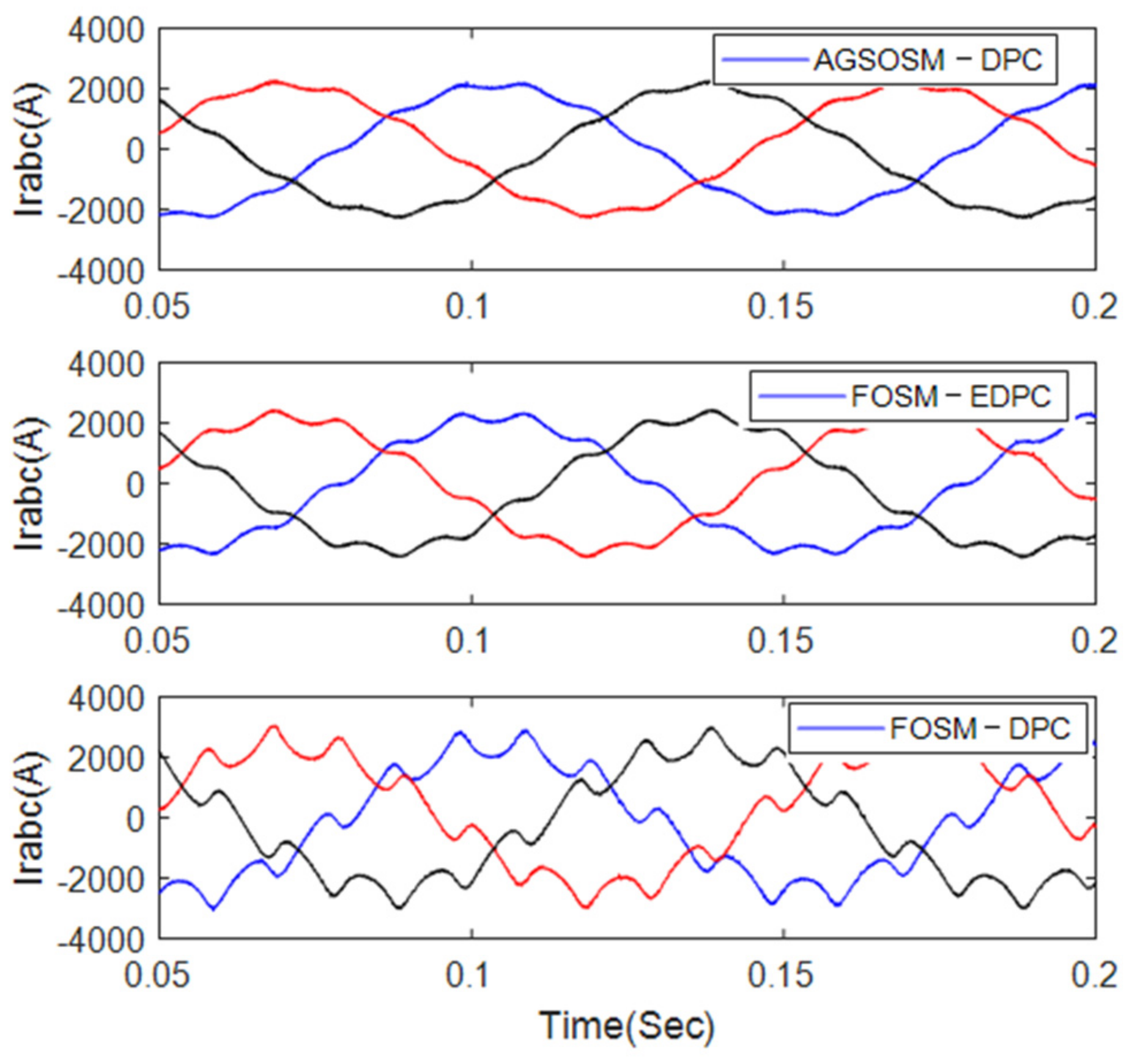
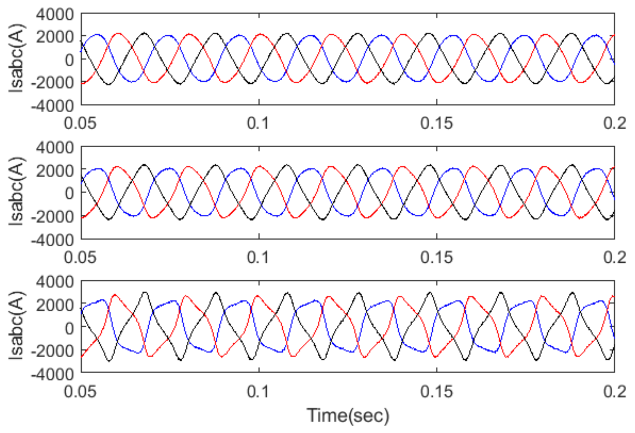
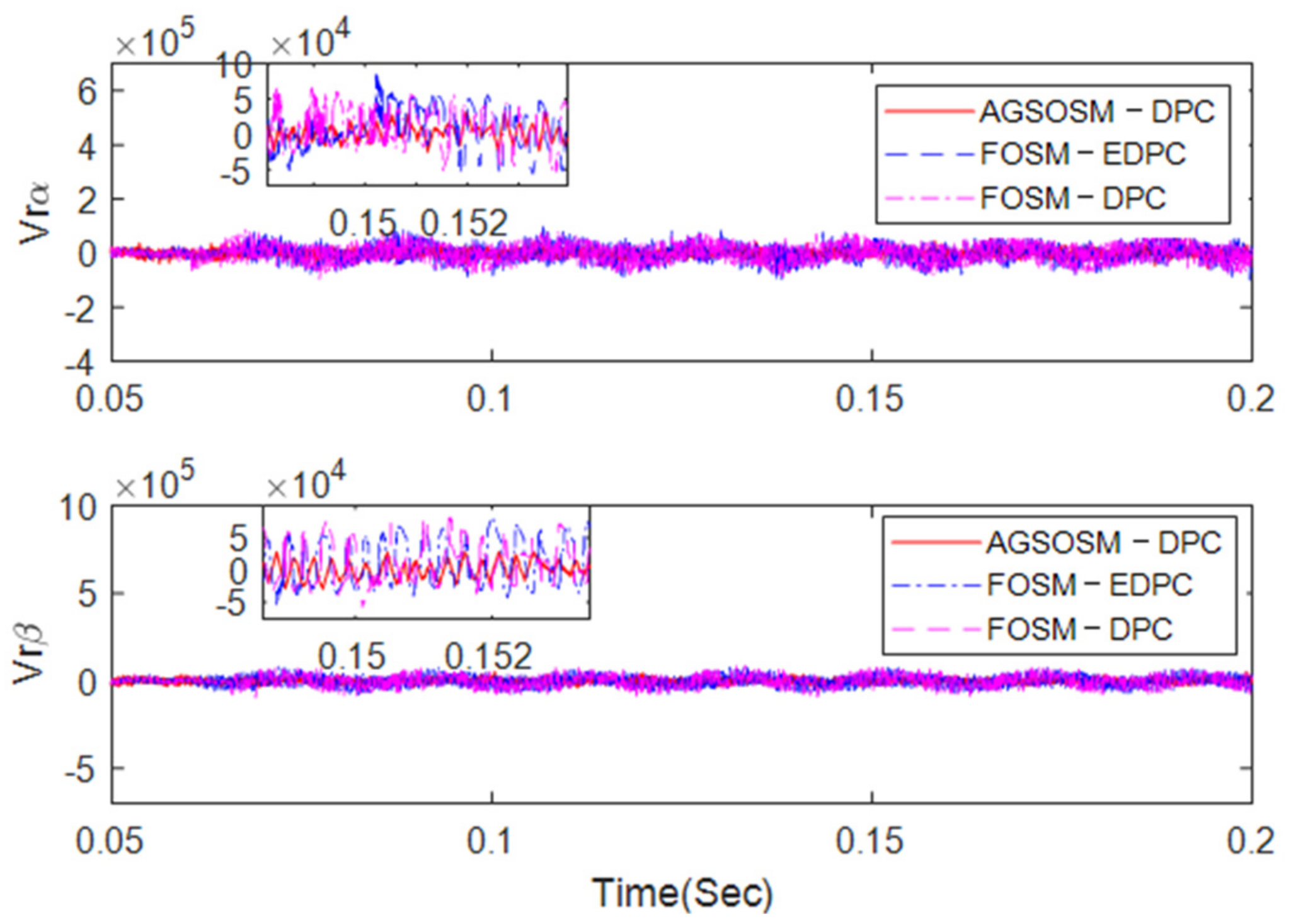
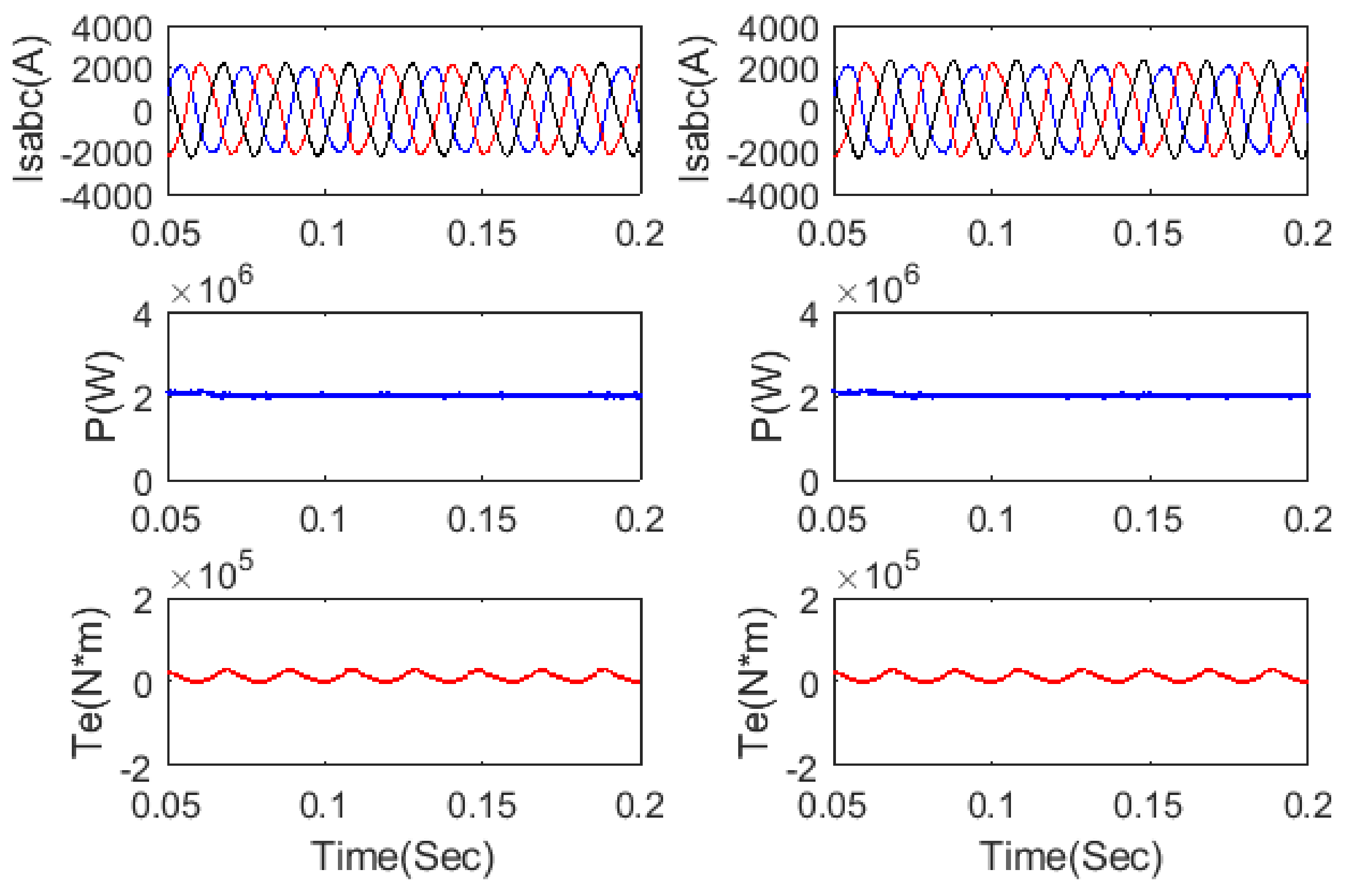
4.2. Simulation Experiment
5. Conclusions
Author Contributions
Funding
Conflicts of Interest
Nomenclature
| Stator, rotor voltage vectors. | |
| Stator, rotor current vectors. | |
| Stator output active and reactive powers. | |
| Stator, rotor flux linkage vectors. | |
| Stator, rotor resistances | |
| Mutual inductance, Stator, rotor self-inductances. | |
| Stator axis |
References
- Djilali, L.; Sanchez, E.N.; Belkheiri, M. Real-time neural sliding mode field oriented control for a DFIG-based wind turbine under balanced and unbalanced grid conditions. IET Renew. Power Gener. 2019, 13, 618–632. [Google Scholar] [CrossRef]
- Available online: https://www.irena.org/ (accessed on 11 August 2019).
- Liu, Y.; Wang, Z.; Xiong, L.; Wang, J.; Jiang, X.; Bai, G.; Li, R.; Liu, S. DFIG wind turbine sliding mode control with exponential reaching law under variable wind speed. Int. J. Electr. Power Energy Syst. 2018, 96, 253–260. [Google Scholar] [CrossRef]
- Xiong, L.; Li, P.; Wu, F.; Ma, M.; Khan, M.W.; Wang, J. A coordinated high-order sliding mode control of DFIG wind turbine for power optimization and grid synchronization. Int. J. Electr. Power Energy Syst. 2019, 105, 679–689. [Google Scholar] [CrossRef]
- Merabet, A.; Eshaft, H.; Tanvir, A.A. Power-current controller based sliding mode control for DFIG-wind energy conversion system. IET Renew. Power Gener. 2018, 12, 1155–1163. [Google Scholar] [CrossRef]
- Yuan, T.; Wang, J.; Guan, Y.; Liu, Z.; Song, X.; Che, Y.; Cao, W. Virtual Inertia Adaptive Control of a Doubly Fed Induction Generator (DFIG) Wind Power System with Hydrogen Energy Storage. Energies 2018, 11, 904. [Google Scholar] [CrossRef]
- Villanueva, I.; Rosales, A.; Ponce, P.; Molina, A. Grid-voltage-oriented sliding mode control for DFIG under balanced and unbalanced grid Faults. IEEE Trans. Sustain. Energy 2018, 9, 1090–1098. [Google Scholar] [CrossRef]
- Nian, H.; Cheng, P.; Zhu, Z.Q. Coordinated direct power control of DFIG system without phase-locked loop under unbalanced grid voltage conditions. IEEE Trans. Power Electron. 2015, 31, 2905–2918. [Google Scholar] [CrossRef]
- Cheng, P.; Nian, H.; Wu, C.; Zhu, Z.Q. Direct stator current vector control strategy of DFIG without phase-locked loop during network unbalance. IEEE Trans. Power Electron. 2016, 32, 284–297. [Google Scholar] [CrossRef]
- Ayyarao, T.S.L.V. Modified vector controlled DFIG wind energy system based on barrier function adaptive sliding mode control. Prot. Control Mod. Power Syst. 2019, 4, 4. [Google Scholar] [CrossRef]
- Mehdipour, C.; Hajizadeh, A.; Mehdipour, I. Dynamic modeling and control of DFIG-based wind turbines under balanced network conditions. Int. J. Electr. Power Energy Syst. 2016, 83, 560–569. [Google Scholar] [CrossRef]
- Bektache, A.; Boukhezzar, B. Nonlinear predictive control of a DFIG-based wind turbine for power capture optimization. Int. J. Electr. Power Energy Syst. 2018, 101, 92–102. [Google Scholar] [CrossRef]
- Alsmadi, Y.M.; Xu, L.; Blaabjerg, F.; Ortega, A.J.; Abdelaziz, A.Y.; Wang, A.; Albataineh, Z. Detailed investigation and performance improvement of the dynamic behavior of grid-connected DFIG-based wind turbines under LVRT conditions. IEEE Trans. Ind. Appl. 2018, 54, 4795–4812. [Google Scholar] [CrossRef]
- Kashkooli, M.R.A.; Madani, S.M.; Lipo, T.A. Improved Direct Torque Control for a DFIG under Symmetrical Voltage Dip with Transient Flux Damping. IEEE Trans. Ind. Electron. 2019. [Google Scholar] [CrossRef]
- Xu, L.; Cartwright, P. Direct active and reactive power control of DFIG for wind energy generation. IEEE Trans. Energy Conver. 2006, 21, 750–758. [Google Scholar] [CrossRef]
- Zandzadeh, M.J.; Vahedi, A. Modeling and improvement of direct power control of DFIG under unbalanced grid voltage condition. Int. J. Electr. Power Energy Syst. 2014, 59, 58–65. [Google Scholar] [CrossRef]
- Debouza, M.; Al-Durra, A.; Errouissi, R.; Muyeen, S.M. Direct power control for grid-connected doubly fed induction generator using disturbance observer based control. Renew. Energy 2018, 125, 365–372. [Google Scholar] [CrossRef]
- Zhang, Y.; Jiao, J.; Xu, D. Direct Power Control of Doubly Fed Induction Generator Using Extended Power Theory Under Unbalanced Network. IEEE Trans. Power Electron. 2019. [Google Scholar] [CrossRef]
- Benamor, A.; Benchouia, M.T.; Srairi, K.; Benbouzid, M.E. A novel rooted tree optimization apply in the high order sliding mode control using super-twisting algorithm based on DTC scheme for DFIG. Int. J. Electr. Power Energy Syst. 2019, 108, 293–302. [Google Scholar] [CrossRef]
- Han, Y.; Ma, R.; Cui, J. Adaptive higher-order sliding mode control for islanding and grid-connected operation of a microgrid. Energies 2018, 11, 1459. [Google Scholar] [CrossRef]
- Mystkowski, A. Lyapunov sliding-mode observers with application for active magnetic bearing operated with zero-bias flux. J. Dyn. Sys. Meas. Control 2019, 141, 041006. [Google Scholar] [CrossRef]
- Hu, J.; Nian, H.; Hu, B.; He, Y.; Zhu, Z.Q. Direct active and reactive power regulation of DFIG using sliding-mode control approach. IEEE Trans. Energy Convers. 2010, 25, 1028–1039. [Google Scholar] [CrossRef]
- Shang, L.; Hu, J. Sliding-mode-based direct power control of grid-connected wind-turbine-driven doubly fed induction generators under unbalanced grid voltage conditions. IEEE Trans. Energy Convers. 2012, 27, 362–373. [Google Scholar] [CrossRef]
- Li, S.; Wang, H.; Tian, Y.; Aitouch, A.; Klein, J. Direct power control of DFIG wind turbine systems based on an intelligent proportional-integral sliding mode control. ISA Trans. 2016, 64, 431–439. [Google Scholar] [CrossRef] [PubMed]
- Sun, D.; Wang, X.; Nian, H.; Zhu, Z.Q. A sliding-mode direct power control strategy for DFIG under both balanced and unbalanced grid conditions using extended active power. IEEE Trans. Power Electron. 2017, 33, 1313–1322. [Google Scholar] [CrossRef]
- Martinez, M.I.; Susperregui, A.; Tapia, G.; Xu, L. Sliding-mode control of a wind turbine-driven double-fed induction generator under non-ideal grid voltages. IET Renew. Power Gener. 2013, 7, 370–379. [Google Scholar] [CrossRef]
- Martinez, M.I.; Tapia, G.; Susperregui, A.; Camblong, H. Sliding-mode control for DFIG rotor-and grid-side converters under unbalanced and harmonically distorted grid voltage. IEEE Trans. Energy Convers. 2012, 27, 328–339. [Google Scholar] [CrossRef]
- Liu, X.; Han, Y.; Wang, C. Second-order sliding mode control for power optimisation of DFIG-based variable speed wind turbine. IET Renew. Power Gener. 2016, 11, 408–418. [Google Scholar] [CrossRef]
- Behera, A.K.; Chalanga, A.; Bandyopadhyay, B. A new geometric proof of super-twisting control with actuator saturation. Automatica 2018, 87, 437–441. [Google Scholar] [CrossRef]
- Beltran, B.; Benbouzid, M.E.H.; Ahmed-Ali, T. Second-order sliding mode control of a doubly fed induction generator driven wind turbine. IEEE Trans. Energy Convers. 2012, 27, 261–269. [Google Scholar] [CrossRef]
- Benbouzid, M.; Beltran, B.; Amirat, Y.; Yao, G.; Han, J.; Mangel, H. Second-order sliding mode control for DFIG-based wind turbines fault ride-through capability enhancement. ISA Trans. 2014, 53, 827–833. [Google Scholar] [CrossRef]
- Evangelista, C.; Puleston, P.; Valenciaga, F.; Fridman, L.M. Lyapunov-designed super-twisting sliding mode control for wind energy conversion optimization. IEEE Trans. Ind. Electron. 2012, 60, 538–545. [Google Scholar] [CrossRef]
- Susperregui, A.; Martinez, M.I.; Zubia, I.; Tapia, G. Design and tuning of fixed-switching-frequency second-order sliding-mode controller for doubly fed induction generator power control. IET Electr. Power Appl. 2012, 6, 696–706. [Google Scholar] [CrossRef]
- Susperregui, A.; Martinez, M.I.; Tapia, G.; Vechiu, I. Second-order sliding-mode controller design and tuning for grid synchronisation and power control of a wind turbine-driven doubly fed induction generator. IET Renew. Power Gener. 2013, 7, 540–551. [Google Scholar] [CrossRef]
- Martinez, M.I.; Susperregui, A.; Tapia, G. Second-order sliding-mode-based global control scheme for wind turbine-driven DFIGs subject to unbalanced and distorted grid voltage. IET Electr. Power Appl. 2017, 11, 1013–1022. [Google Scholar] [CrossRef]
- Shah, A.P.; Mehta, A.J. Direct power control of DFIG using super-twisting algorithm based on second-order sliding mode control. In Proceedings of the 2016 14th International Workshop on Variable Structure Systems (VSS), Nanjing, China, 1–4 June 2016; pp. 136–141. [Google Scholar] [CrossRef]
- Shah, A.P.; Mehta, A.J. Direct power control of grid-connected DFIG using variable gain super-twisting sliding mode controller for wind energy optimization. In Proceedings of the IECON 2017-43rd Annual Conference of the IEEE Industrial Electronics Society, Beijing, China, 29 October–1 November 2017; pp. 2448–2454. [Google Scholar] [CrossRef]
- Zhang, Y.; Qu, C. Direct power control of a pulse width modulation rectifier using space vector modulation under unbalanced grid voltages. IEEE Trans. Power Electron. 2014, 30, 5892–5901. [Google Scholar] [CrossRef]
- Seeber, R.; Horn, M. Stability proof for a well-established super-twisting parameter setting. Automatica 2017, 84, 241–243. [Google Scholar] [CrossRef]


| Rated Power (MW) | 2 |
| Line-to-line voltage (rms)(V) | 690 |
| Stator frequency (Hz) | 50 |
| Stator-to-rotor ratio | 3 |
| Rs (ohm) | 0.001518 |
| Rr (ohm) | 0.002087 |
| Ls (mH) | 0.059906 |
| Lr (mH) | 0.08206 |
| Lm (mH) | 2.4 |
| Pole pairs | 2 |
| Lumped inertia constant (kg·m2) | 17.23 |
| Control Strategy | Transitory r Response (ms) | Power Ripple (%) | THD (%) | |||
|---|---|---|---|---|---|---|
| P | Q | P | Q | Is | Ir | |
| AGSOSM-DPC | 1.3 | 1.6 | 12.7 | 17.4 | 1.9 | 2.7 |
| FOSM-EDPC | 1.3 | 1.7 | 15.3 | 19.7 | 2.3 | 3.2 |
| FOSM-DPC | 1.5 | 2.1 | 19.5 | 21.2 | 5.2 | 6.1 |
© 2019 by the authors. Licensee MDPI, Basel, Switzerland. This article is an open access article distributed under the terms and conditions of the Creative Commons Attribution (CC BY) license (http://creativecommons.org/licenses/by/4.0/).
Share and Cite
Han, Y.; Ma, R. Adaptive-Gain Second-Order Sliding Mode Direct Power Control for Wind-Turbine-Driven DFIG under Balanced and Unbalanced Grid Voltage. Energies 2019, 12, 3886. https://doi.org/10.3390/en12203886
Han Y, Ma R. Adaptive-Gain Second-Order Sliding Mode Direct Power Control for Wind-Turbine-Driven DFIG under Balanced and Unbalanced Grid Voltage. Energies. 2019; 12(20):3886. https://doi.org/10.3390/en12203886
Chicago/Turabian StyleHan, Yaozhen, and Ronglin Ma. 2019. "Adaptive-Gain Second-Order Sliding Mode Direct Power Control for Wind-Turbine-Driven DFIG under Balanced and Unbalanced Grid Voltage" Energies 12, no. 20: 3886. https://doi.org/10.3390/en12203886
APA StyleHan, Y., & Ma, R. (2019). Adaptive-Gain Second-Order Sliding Mode Direct Power Control for Wind-Turbine-Driven DFIG under Balanced and Unbalanced Grid Voltage. Energies, 12(20), 3886. https://doi.org/10.3390/en12203886