Experimental and Numerical Analysis of a Seawall’s Effect on Wind Turbine Performance

Abstract

For the purposes of this study, a wind tunnel experiment and a numerical analysis during ebb and high tides were conducted to determine the positive and negative effects of wind flow influenced by a seawall structure on the performance of wind turbines installed along a coastal seawall. The comparison of the wind flow field between a wind tunnel experiment performed with a 1/100 scale model and a computational fluid dynamics (CFD) analysis confirmed that the MP k-turbulence model estimated flow separation on the leeside of the seawall the most accurately. The CFD analysis verified that wind speed-up occurred due to the virtual hill effect caused by the seawall’s windward slope and the recirculation zone of its rear face, which created a positive effect by mitigating wind shear while increasing the mean wind speed in the wind turbine’s rotor plane. In contrast, the turbulence effect of flow separation on the seawall’s leeside was limited to the area below the wind turbine rotor, and had no negative effect. The use of the CFD verified with the comparison with the wind tunnel experiment was extended to the full-scale seawall, and the results of the analysis based on the wind turbine Supervisory Control and Data Acquisition (SCADA) data of a wind farm confirmed that the seawall effect was equivalent to a 1.5% increase in power generation as a result of a mitigation of the wind profile.

1. Introduction

Currently, there are about 100 wind farms in South Korea, of which 60% are located in high mountainous regions, 30% are located in coastal areas, and 10% are located in inland plains [1]. In general, as terrain becomes higher, wind speed increases, which is advantageous to wind power generation. However, complex mountainous terrain is accompanied by strong gusts of wind and turbulence, which means that wind turbines require greater structural strength.

Most coastal wind farms in South Korea are on the west coast where the prevailing wind direction matches the sea breeze, which makes it possible to use both synoptic wind and sea breeze simultaneously according to the wind zone classification [2]. Among the wind farms built along the west coast, wind turbines were only installed on the inner side of the coastal seawall at the Gunsan and Saemangeum wind farms, as shown in Figure 1.

However, since a seawall is a coastal defense structure that blocks waves, deformation in the wind field occurs as the sea breeze passes over the sea-facing slope of the seawall. According to the Korean patent by Kim and Jang [3], if a virtual hill is made by inducing flow separation, such as a fence upwind of the wind turbines [4], wind speed-up occurs and wind shear is mitigated, thereby producing a positive effect on wind turbine performance [5]. Thus, seawalls may have a positive effect on wind power generation, although a negative effect, such as an increase in the fatigue load on wind turbine blades, may also occur due to higher turbulence intensity or intermittent flow separation on the leeside of the seawall.

Bitsuamlak comprehensively reviewed the previous studies on computational fluid dynamics (CFD) and wind tunnel tests of speed-up due to an escarpment or seawall [6]. Barthelmie measured an increase of wind speed and turbulence intensity over a two-dimensional (2D) cliff, and compared them with WAsP (Wind Atlas Analysis and Application Program) and WAsP CFD [7]. Tobin and Chamorro analyzed the principle of increasing power generation by inducing an acceleration of wind speed by installing a windbreak in front of a wind turbine using the Integrated Boundary Layer Theory [8]. However, the idea of inducing an acceleration of wind speed by installing a structure on the windward side of a wind turbine has been patented in Korea by the author [3].

In order to design a wind farm, it is necessary to identify the spatial distribution of wind speed in a wind resource assessment in which wind fields of at least 16 or more directions should be simulated using a flow model [9]. A mathematical model that linearizes the Reynolds-averaged Navier–Stokes (RANS) equation has been widely used as a flow model in wind resource assessments (e.g., WAsP, Openwind). However, due to the competitive cost-effectiveness of CFD as a result of rapid improvements of computational power, the trend has recently switched to the use of CFD based on steady-state RANS and two-equation turbulence models (e.g., WindSim, Meteordyn WT, WAsP CFD). It is well-known that the CFD-based flow models showed better performance than the mathematical models in complex terrain [10]. On the other hand, it is still too early to use large-eddy simulations (LES) or direct numerical simulations (DNS), which basically require extensive transient three-dimensional (3D) computation in a very fine mesh, in a wind farm design where iterations of numerous cases are essential to securing the optimum design.

Although studies on LES analysis in real terrain have been published in recent years, their results were still at the academic research stage in that they compared a wind tunnel experiment or the RANS results of basic simple terrain such as 2D hills, a single 3D hill, etc. [11,12]. The round robin test of Bolund Hill, which was a comprehensive benchmark for the flow models used in the design of wind farms, assessed that the results obtained by LES were not very reliable compared to those obtained by RANS [13]. In the case where LES was applied to the Cape Noma Wind Farm in Japan, the prediction error of wind speed was around 20%, which indicates that LES is not yet sufficiently advanced to be confidently used at the worksites of wind resource assessments [14].

Another drawback of LES analysis in real terrain is that it is difficult to set up an upstream boundary condition, which also significantly affects the results of any analysis. In other words, with RANS, the field or wind tunnel measurements can be directly imposed as an upstream boundary condition, whereas with LES, it is necessary to perform an auxiliary simulation of boundary layer development either by a virtual wind tunnel simulation technique, including the boundary layer development stage [12,15], or by using a recycling method, until the wind profile becomes the same as that of the upstream profile of the field or wind tunnel measurements [16,17].

In this study, the RANS-based CFD and two-equation turbulence models were used to determine the positive or negative effects on the wind turbine performance of flow field deformation caused by seawalls. Since the wind turbines are arranged in a row along the seawall, they were regarded as 2D, so a semi-2D CFD analysis was conducted. In addition, wind tunnel experiments were performed to confirm the reliability of the CFD analysis.

2. Data and Methods

2.1. Analysis Procedure

The wind tunnel experiment and CFD analysis were performed according to the procedure shown in Figure 2 in order to analyze the deformation of the wind flow field due to the seawall, and to evaluate the wind turbines’ performance.

The first step consisted of a downscaled model analysis.

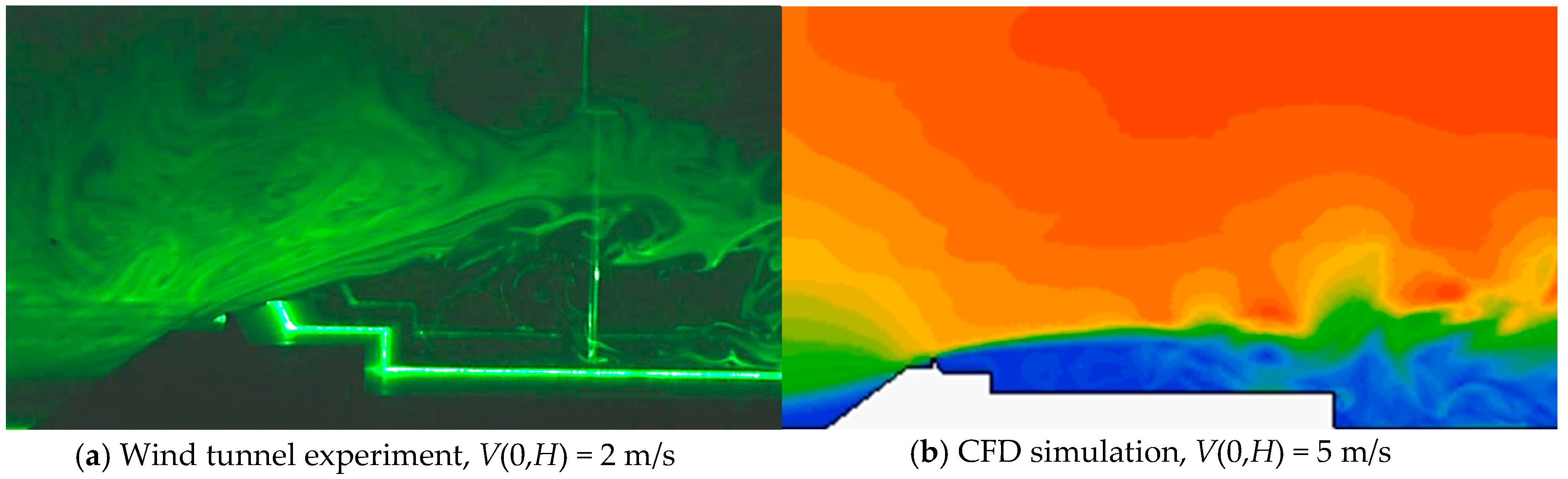
• First, a wind tunnel experiment was conducted using a downscaled model (1/100) of the Gunsan wind farm on the west coast of South Korea. Through this, how the atmospheric boundary layer of downwind was deformed by the seawall structure located in the upwind of the wind turbine was experimentally investigated.
• Next, a semi-2D CFD analysis of the same dimensions and flow conditions as those of the model used in the wind tunnel experiment was conducted. In this analysis, a number of turbulence models were tested, and the model that proved to be most effective in analyzing the flow separation-accompanied turbulent wind flow was selected.

In the second step, the analysis was extended to the full-scale seawall using the CFD, whose reliability had previously been confirmed through an interverification of the downscaled model with the wind tunnel experiment.

• First, a CFD analysis was conducted using the full-scale seawall to overcome the limitation of the Reynolds number similarity in the wind tunnel experiment, and to verify whether the seawall had the same positive and negative effects as those seen in the analysis of the full-scale seawall.
• Finally, the Supervisory Control and Data Acquisition (SCADA) data of the Gunsan wind farm were analyzed to verify the wind shear mitigation effects, which were confirmed by the wind tunnel experiment and CFD simulation. That is, the hypothesis that the seawall would increase power generation if there was a difference in power generation made during westerly wind, which is the sea breeze, and easterly wind, the opposite wind direction, was quantitatively and practically verified.

In wind engineering, the CFD of wind flow over/around a terrain or a structure with a high Reynolds number must be accompanied by a wind tunnel experiment due to the high uncertainty of CFD prediction, particularly when flow separation is involved. Once the CFD simulation has been compared and verified by comparing it with a wind tunnel experiment according to the same procedure as that used in this study, the full scale can be analyzed using the verified CFD, thereby having a process of projection of wind tunnel experiments into the full-scale application [18]. This analysis procedure is the same as that used in aerodynamic modeling in such fields as airplane design, vehicle design, and so forth [19].

2.2. Wind Tunnel Experiment

2.2.1. Wind Conditions at the Gunsan Wind Farm

The wind tunnel experiment was conducted after manufacturing a downscaled model of the Gunsan wind farm (35.9540° N, 126.5232° E) located on the rear side of the coastal seawall inside the Gunjang National Industrial Complex in Gunsan, Jeollabuk-do, South Korea. The Gunsan wind farm consists of a row of 10 wind turbines spaced at intervals of 200 m along the seawall in the south–north direction, as shown in Figure 1. Six of the turbines are NEG-Micon NM48 750 kW (hub height, H: 45 m, blade length: 48 m) turbines, while the other four are Vestas V52 850 kW (hub height: 49 m, blade length: 52 m).

According to the Korea wind map developed by the Korea Institute of Energy Research [20], the main wind direction of the Gunsan wind farm region is north–northwest, and the mean wind speed at 50 m above the ground is 5.4 m/s, and the wind profile exponent (α) is 0.13. For reference, the wind speed profile V(z) can be represented by the following equation:

$$\frac{V\left(z\right)}{V\left(H\right)}={\left(\frac{z}{H}\right)}^{\alpha }$$

(1)

2.2.2. Simulated Wind Condition in the Wind Tunnel

The wind tunnel experiment was conducted in an Eiffel-type boundary layer wind tunnel at the Kumoh National Institute of Technology under the following conditions: a contraction ratio of 4:1, and a test section of 1.5 m (width) × 1.3 m (height) × 17 m (length) [21]. The exposure category D, which corresponds to an offshore proposed by the Korea Building Code-Structural [22], was simulated with roughness blocks arranged on the floor and spires installed at the entry of the test section, which was fully consistent with the wind profile exponent (0.13) of the location provided on the Korea wind map.

Figure 3 shows the boundary layer wind profiles in the test section of the wind tunnel, which illustrate the mean wind speed and the turbulence intensity, respectively. In this figure, the vertical axis represents the height above ground, which is non-dimensionalized with the hub height (H) of the wind turbine.

In addition to the similarity between the mean wind speed profile and the turbulence intensity profile, similarity with the turbulence structure should be satisfied when simulating the atmospheric boundary layer in the wind tunnel. Figure 4 shows a comparison of the non-dimensional power spectrum density of the wind flow reproduced in the wind tunnel and von Karman’s empirical equation [23]. As shown in the graph, the decaying structure of the wind power spectrum was reproduced similarly to that of natural wind. In the graph, n refers to frequency (Hz), and n* refers to non-dimensional frequency.

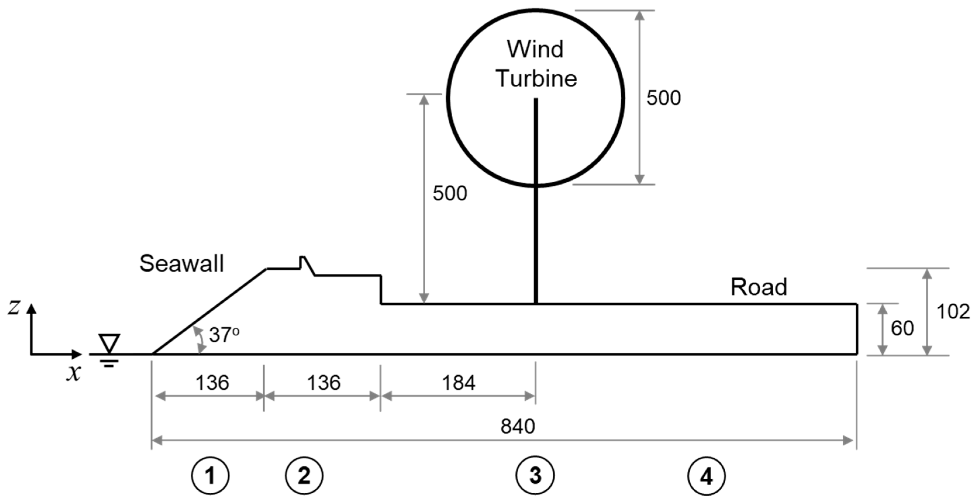
2.2.3. Downscaled Seawall Model

A 1/100 scale model was employed after considering the blockage effect (<10%) caused by a model in the test section. The dimensions of the downscaled seawall model are shown in Figure 5. The wind speed was measured every 30 s with a sampling rate of 200 Hz using a hot-wire anemometer, and was scanned every 25 mm in the vertical direction at the locations marked with a circle number, as shown in Figure 5. The measurements were repeated five times, and the average was taken.

A hub height of 50 m in the full-scale wind turbine was corresponded to 500 mm in the downscaled model; the mean wind speed at this height was 5 m/s, the wind profile exponent was 0.13, and the turbulence intensity in the lower part of the boundary layer was set to 12%.

For the seawall model, two models were manufactured for high and ebb tide events, respectively, in consideration of the tidal range (maximum 7 m) in the Gunsan region, tetrapods were installed on the sloping surface facing the sea (see Figure 1), and, in consideration of this, equivalent roughness was manufactured on the surface of the slope. In addition, three seawall incident angles (0°, 11.25°, and 22.5°) were used in the experiment. Since the incident angle was defined by an angle made by the x-axis and the wind vector, Figure 6 shows a 0° of incident angle setting.

The test objects normally discussed in civil wind engineering have a very large characteristic length. Thus, when wind tunnel experiments are conducted with a model whose downscaled ratio is large, i.e., 100 times or 1000 times larger, then a Reynolds number mismatch occurs. However, when flow separation occurs in a turbulent flow whose Reynolds number is more than 10⁴, the Reynolds number dependency may be ignored in general [24]. For reference, the Reynolds number of the present wind tunnel experiment is 1.7 × 10⁵.

2.3. Wind Tunnel Experiment

The wind flow field over the seawall was simulated by solving the RANS equation using the CFD software Cradle SC/Tetra v12. SC/Tetra, which is a commercial flow solver based on a finite volume method that employs the SIMPLEC (Semi-Implicit Method for Pressure Linked Equations-Consistent) algorithm for pressure–velocity coupling and the second-order QUICK upwind scheme for convection terms. Considering the geometrical characteristics of the seawall, which extends in a straight line in the south–north direction, semi-2D simulations were conducted, and an unstructured grid for numerical analysis was configured, as shown in Figure 7.

In general, when a hill’s slope exceeds 20°, flow separation is likely to occur on the lee side [25], and even more so in angled structures, as can be seen at the upper end of the seawall. In cases where atmospheric wind flows accompanied by flow separation are analyzed using CFD, accuracy may vary considerably depending on which turbulence model is used. Thus, it is important to select a suitable turbulence model. This study tested the standard k-ε, RNG k-ε, modified production (MP) k-ε, and realizable k-ε, models, and evaluated which turbulence model best matched the results of the wind tunnel experiment.

The same computational domain and boundary conditions were applied to the CFD of the downscaled model as those applied to the test section in the wind tunnel experiment. That is, a 3 H space in the upwind direction and a 9 H space in the downwind direction from the wind turbine were put in place; while for the top boundary, a domain of 2.6 H (1.3 m), which was up to the wind tunnel upper wall, was set. On the other hand, a pressure boundary condition instead of a no-slip condition was applied to the top boundary condition in the case of the full-scale CFD so as to allow outflow.

If the incident angle was not 0°, a periodic boundary condition was applied in the y-axis direction, which was the width direction of the seawall, thereby conducting semi-2D CFD that allowed the y-directional wind vector.

2.4. Wind Farm SCADA Data

A virtual hill effect occurs due to the flow separation generated at the top of the seawall when a sea breeze passes over the seawall structure. The wind flow passing over the virtual hill generates wind shear mitigation and speed-up at the hilltop, which in turn increases wind power generation. For reference, the speed-up ratio (SR) was defined as follows [26]:

$$SR=\frac{V\left(x,z\right)-V\left(0,z\right)}{V\left(0,z\right)}$$

(2)

where V(0,z) is the upstream wind speed profile.

To prove the hypothesis that wind power is increased by the seawall, the hourly SCADA data of the Gunsan wind farm were utilized. The construction of the Gunsan wind farm was completed in 2007. Then, the inner side of the seawall, i.e., the east side, underwent reclamation work and development from 2009, which changed the ground conditions. Thus, the verification period was limited to 2008, which was less influenced by external conditions.

The wind direction was divided into two: westerly wind (270° ± 45°), where the wind profile mitigation and speed-up was expected, and the opposite easterly wind (90° ± 45°), in order to compare the power generation difference, which was then analyzed by wind speed bins. That is, the power-up ratio (PR) was defined as follows:

$$PR=\frac{\mathsf{\Delta }P\left(V\right)}{P_i\left(V\right)}=\frac{P\left(V,\mathrm{westerly}\right)-P\left(V,\mathrm{easterly}\right)}{P_i\left(V\right)}$$

(3)

Note that only the quasi steady-state where wind speed was maintained within a ±10% change for more than three hours was singled out. P_i(V) refers to the theoretical power generation (kW) that is calculated by the wind turbine power curve when the wind speed is V (m/s) which is measured by the nacelle anemometry of the wind turbine.

Hence, a nacelle anemometer installed on wind turbines measures the wind speed incident to the wind turbine hub V(0,H), so it is not possible to know whether the speed-up occurred or not. In order to identify the speed-up caused by the seawall, the wind speeds should also be measured simultaneously not only at the wind turbine position V(0,H), but also at the far upstream position V(−$\infty$,H).

Even if the wind speeds measured by the nacelle anemometer are the same, the wind profiles incident to the wind turbine rotor would be different. That is, in case of the westerly wind, wind shear mitigation occurs due to the seawall effect, while the easterly wind has an unmodified far-upstream wind profile. Therefore, the actual power-up ratio can be calculated by Equation (3) using the SCADA data. On the other hand, the theoretical power-up ratio can be calculated using either the wind tunnel experiments or the CFD simulation results.

In order to calculate the power generation by different wind profiles, the rotor-equivalent wind speed (REWS) should be used instead of the hub-height wind speed [27,28]. In the present study, the theoretical power-up ratio was calculated using the CFD simulation results where the hub-height wind speeds of the westerly and easterly winds were set to equal to make it the same condition as the SCADA data analysis.

3. Results and Discussion

3.1. Downscaled Model Validation

Figure 8 shows the results of the CFD analysis of the 1/100 scale model, in which upward wind was attracted to the sloping side of the seawall, resulting in flow separation at the top, thereby showing a rapid rise of turbulent kinetic energy. Furthermore, wind speed-up was generated along the upper top of the sloping side. In particular, the figure verified that the wind speed-up was significantly higher at the lower part of the wind speed profile.

To verify the accuracy of the CFD simulation and select a suitable turbulence model for the turbulent flow simulation, their results were compared with the results of the wind tunnel experiment. Figure 9 shows the comparison of the vertical wind speed profile and the turbulence intensity profile at the measurement locations marked on Figure 5 during ebb tide, when the incident angle was 0°.

The wind speed profiles were compared first. Most turbulence models over-estimated the wind speed at ① the slope of the seawall, and this trend was also revealed at ② the top of the seawall. However, the MP k-ε model exhibited almost the same prediction results as those of the wind tunnel measurements. ③ At the wind turbine installation location and ④ the rear side, most turbulence models predicted flow separation very well, with the standard k-ε model giving the least accurate predictions.

Next, the turbulent intensity profiles were compared, the results of which are as follows: Overall, the standard k-ε model over-estimated the turbulent kinetic energy. In contrast, the MP k-ε model, in which the Kato–Launder limiter was applied to prevent excessive production of the strain rate in the stagnation region, was evaluated as the best model in all of the measurement locations [29].

The comparison with the wind tunnel experiment showed that the CFD simulation, in which the MP k-ε turbulence model was used, predicted both the mean wind speed profile and the turbulence intensity profile very accurately. Figure 10 shows a comparison of the results of the analysis using the MP k-ε model in the case of high tide with those of the wind tunnel experiment when the incident angle was 0°, 11.25°, and 22.5°. The change due to an increase in the incident angle rarely seen not only the wind speed profile, but also the turbulent intensity profile. However, the figure verified that the x-directional momentum decreased as the incident angle increased, shortening the length of the recirculation zone.

Figure 11 shows a visualization of the flow separation and recirculation characteristics, in which the wind tunnel experiment result was shot by making a laser sheet and spraying smoke, and the CFD results were the outcome of the LES. In both cases, it was confirmed that the size and height of the recirculation zone, whose turbulence intensity increased rapidly due to turbulence mixing, were not enough to influence the wind turbine blades, as their height was only 1/4 that of the wind turbine hub height. For reference, the scale of the seawall model in Figure 11a was 1/100, while that of the wind turbine model was 1/200. Thus, great care should be taken not to misunderstand the size of the recirculation zone.

3.2. Full-Scale Model Validation

The results of the CFD, whose reliability was validated by a comparative validation with that of the wind tunnel experiment, and which was then applied to the full-scale simulation, are shown in Figure 12. In the wind tunnel experiment, the seawall model was made with a finite length, which made a difference that there was a backward step. However, the mean wind speed showed no significant qualitative difference according to the scale-up.

Figure 13 shows a comparison of the mean wind speed profile and the turbulence intensity profile between the upstream position and the wind turbine position. In the center of the figure, the upper and lower ends of the hub height and rotor plane of the wind turbine are marked with lines. When paying attention to the rotor plane, the mean wind speed shows more speed-up than that of the upstream overall, especially at the lower part. Thus, not only did the wind speed accelerate at the hub height due to the virtual hill effect, but the wind shear was mitigated flat, resulting in a gain in power generation.

In contrast, the turbulence intensity increased significantly only at the recirculation zone, but its height did not exceed the lower end of the rotor plane, while the turbulence intensity at the rotor plane was comparable with that at the upstream.

3.3. Wind Power Augmentation

Table 1. Speed-up ratio (SR) at the hub-height of the wind turbine by incident angle.

Case	0°	11.25°	22.5°
Ebb tide	10.0	8.6	7.6
High tide	7.6	7.4	6.2

presents the summary of the speed-up ratio according to the incident angle of upstream wind at the wind turbine position, and according to high and ebb tides. The values are calculated at the hub height. The speed-up ratio tended to increase as the size of the virtual hill (height and length) increased more at ebb tide than at high tide. On the other hand, the speed-up ratio tended to decrease as the incident angle increased.

Figure 14 proves that the wind shear mitigation caused by the seawall is linked with the increase in wind power generation. The actual power-up ratio at the wind turbine hub height increased by 1.5% on average based on Equation (3) using the SCADA data, while the theoretical power-up ratio estimated by the SCADA data was 1.4%, which are very close to agreement. For reference, the Gunsan wind farm region is a low wind speed zone of wind class 2, so a speed of 10 m/s or stronger is very low.

4. Conclusions

This study aimed to prove the hypothesis that an acceleration of wind speed and wind shear mitigation would occur due to the virtual hill effect caused by the windward slope and the rear end of the recirculation zone when a wind turbine was installed on the inner side of the coastal seawall. To that end, a wind tunnel experiment and a numerical analysis were conducted.

The main results of this study are summarized as follows.

(1)

The comparative validation results of the wind tunnel experiment and the CFD using the downscaled model indicate that the MP k-ε model was the most suitable turbulence model to analyze the wind field, which was accompanied by flow separation.

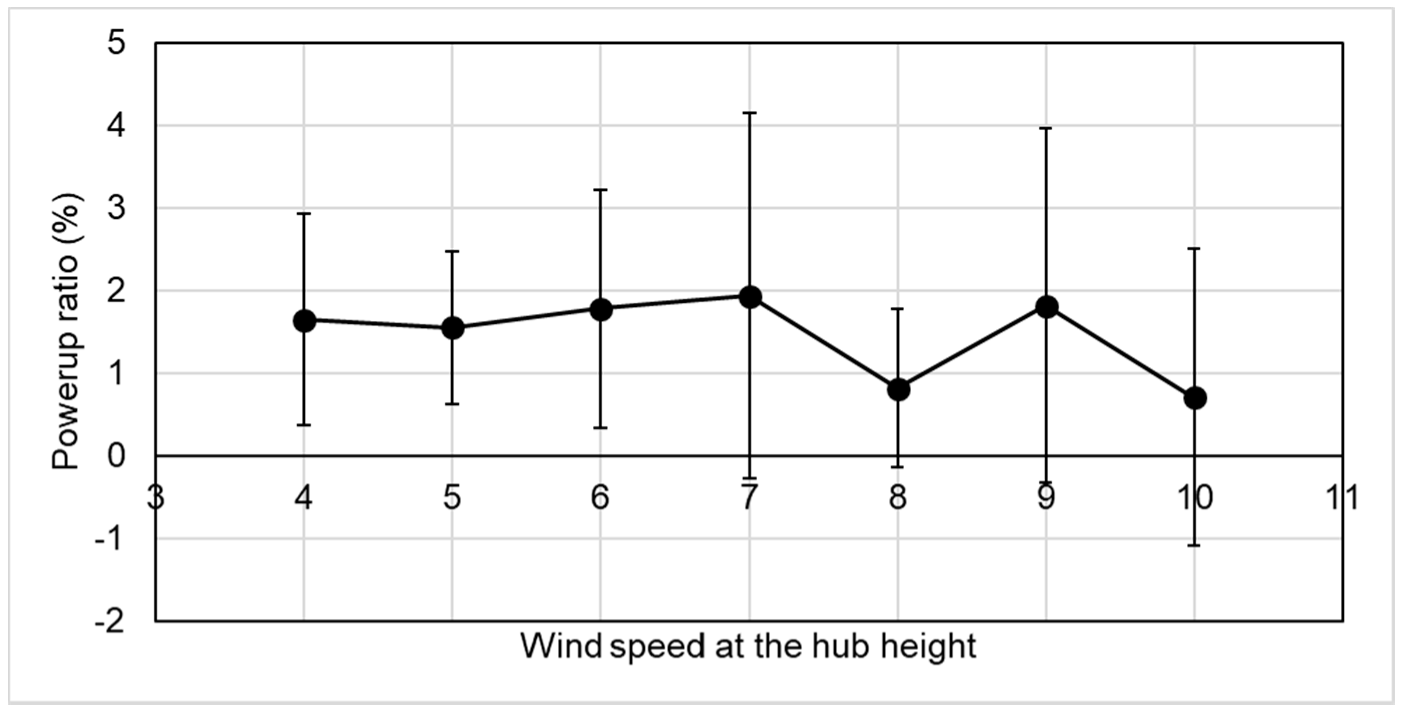
(2)

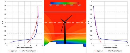
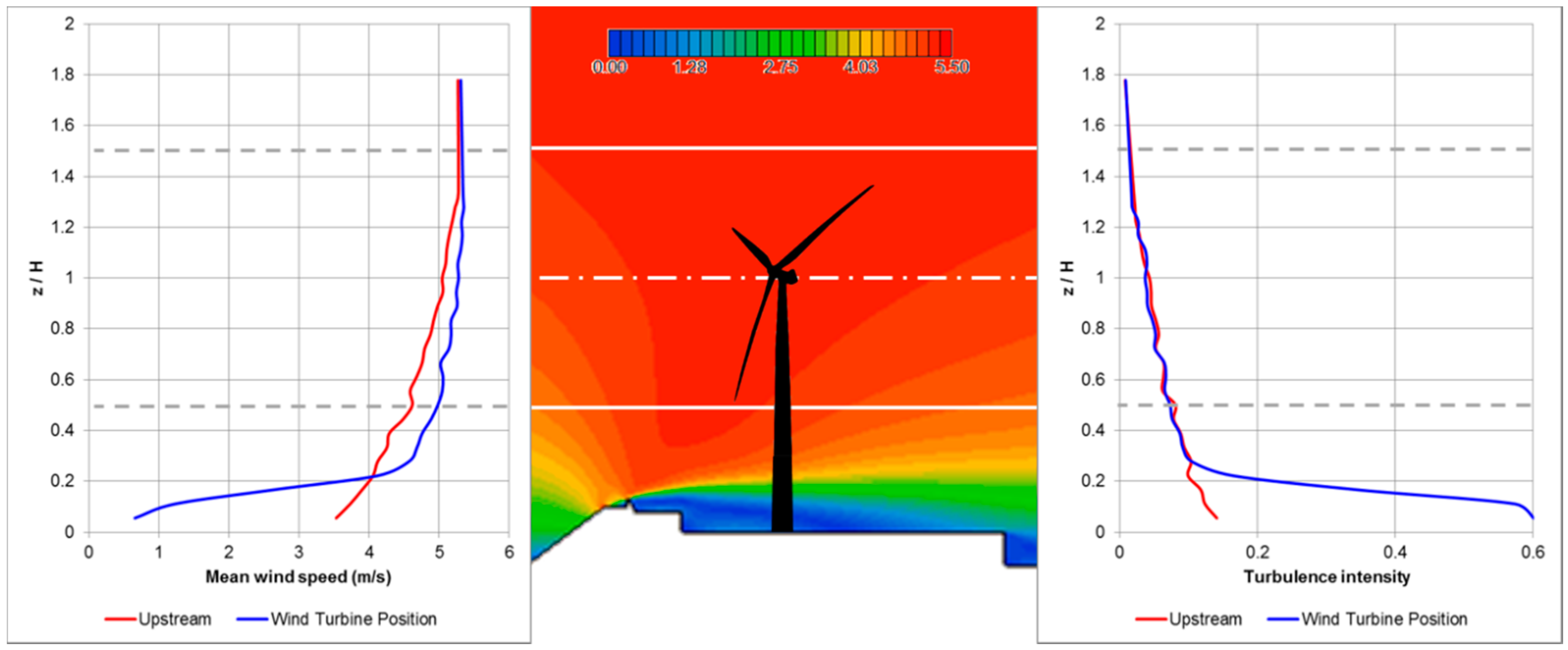
Wind speed-up and wind shear mitigation occurred not only in the wind turbine hub height but also in the entire rotor plane due to the virtual hill effect, which was produced by the seawall slope and the recirculation zone on the rear side of the seawall. Both of them played a role in increasing power generation, and the SCADA data analysis of the Gunsan wind farm confirmed an effect equivalent to an increase in power generation of about 1.5% by a mitigation of the wind profile, which is comparable to the theoretical increase of 1.4% estimated by the wind profiles of CFD simulations.

(3)

The flow separation occurring at the upper top of the seawall rapidly increased the turbulence intensity, but its impact range was lower than 1/4 of the wind turbine hub height, which confirmed that there was no adverse effect on the rotor blades, such as when applying fatigue loads directly.

(4)

If wind farms are developed near civil engineering structures such as seawalls or escarpments in the future, increases in power generation could be achieved by selecting a location where wind speed-up and wind shear mitigation are expected based on the results of this study.

References

1. Kim, H.G.; Kang, Y.H.; Kim, J.Y. Evaluation of wind resource potential in mountainous region considering morphometric terrain characteristics. Wind Eng. 2017, 41, 114–123. [Google Scholar] [CrossRef]
2. Kim, J.S.; Kim, H.G.; Park, H.D. Surface wind regionalization based on similarity of time-series wind vectors. Asian J. Atmos. Environ. 2016, 10, 80–89. [Google Scholar] [CrossRef]
3. Kim, H.G.; Jang, M.S. A Structure for Compensating Wind Velocity. Korea Patent 10-0969595, 5 July 2010. [Google Scholar]
4. Wood, N. The onset of flow separation in neutral, turbulent flow over hills. Bound. Layer Meteorol. 1995, 76, 137–164. [Google Scholar] [CrossRef]
5. Wagner, R.; Cañadillas, B.; Clifton, A.; Feeney, S.; Nygaard, N.; Poodt, M.; St Martin, C.; Tüxen, E.; Wagenaar, J. Rotor equivalent wind speed for power curve measurement—Comparative exercise for IEA Wind Annex 32. J. Phys. Conf. Ser. 2014, 524, 012108. [Google Scholar] [CrossRef]
6. Bitsuamlak, G.T.; Stathopoulos, T.; Bédard, C. Numerical evaluation of wind flow over complex terrain: Review. J. Aerosp. Eng. 2004, 17, 135–145. [Google Scholar] [CrossRef]
7. Barthelmie, R.J.; Wang, H.; Doubrawa, P.; Giroux, G.; Pryor, S.C. Effects of an escarpment on flow parameters of relevance to wind turbines. Wind Energy 2016, 19, 2271–2286. [Google Scholar] [CrossRef]
8. Tobin, N.; Chamorro, L.P. Windbreak effects within infinite wind farms. Energies 2017, 10, 1140. [Google Scholar] [CrossRef]
9. Kim, H.G. A method of accelerating the convergence of computational fluid dynamics for micro-siting wind mapping. Computation 2019, 7, 22. [Google Scholar] [CrossRef]
10. Ramos, D.A.; Guedes, V.G.; Pereira, R.R.S.; Valentim, T.A.S.; Netto, W.A.C. Further considerations on WAsP, OpenWind and WindSim comparison study: Atmospheric flow modelling over complex terrain and energy production estimate. In Proceedings of the Windpower 2017 Conference and Exhibition, Rio De Janeiro, Brazil, 29–31 August 2017. [Google Scholar]
11. Ishihara, T.; Qi, Y. Numerical study of turbulent flow fields over steep terrain by using modified delayed detached-eddy simulations. Bound. Layer Meteorol. 2019, 170, 45–68. [Google Scholar] [CrossRef]
12. Liu, Z.; Cao, S.; Liu, H.; Ishihara, T. Large-eddy simulations of the flow over an isolated three-dimensional hill. Bound. Layer Meteorol. 2019, 170, 415–441. [Google Scholar] [CrossRef]
13. Bechmann, A.; Sørensen, N.N.; Berg, J.; Mann, J.; Réthoré, P.E. The Bolund experiment, Part II: Blind comparison of microscale flow models. Bound. Layer Meteorol. 2011, 141, 245–271. [Google Scholar] [CrossRef]
14. Uchida, T. Computational fluid dynamics approach to predict the actual wind speed over complex terrain. Energies 2018, 11, 1694. [Google Scholar] [CrossRef]
15. Uchida, T. High-resolution LES of terrain-induced turbulence around wind turbine generators by using turbulent inflow boundary conditions. Open J. Fluid Dyn. 2017, 7, 511–524. [Google Scholar] [CrossRef]
16. Conan, B.; Chaudhari, A.; Aubrun, S.; van Beeck, J.; Hämäläinen, J.; Hellsten, A. Experimental and numerical modelling of flow over complex terrain: The Bolund hill. Bound. Layer Meteorol. 2016, 158, 183–208. [Google Scholar] [CrossRef]
17. Chaudhari, A.; Vuorinen, V.; Hämäläinen, J.; Hellsten, A. Large-eddy simulations for hill terrains: Validation with wind-tunnel and field measurements. Comp. Appl. Math. 2018, 37, 2017–2038. [Google Scholar] [CrossRef]
18. Kimura, K. Chapter 3—Wind loads. In Innovative Bridge Design Handbook—Construction, Rehabilitation and Maintenance; Pipinato, A., Ed.; Elsevier: Amsterdam, The Netherlands, 2016; pp. 37–48. [Google Scholar]
19. Cook, M.V. Chapter 12—Aerodynamic modelling. In Flight Dynamics Principles, 3rd ed.; Elsevier: Oxford, UK, 2013; pp. 353–369. [Google Scholar]
20. Korea Institute of Energy Research. Korea Renewable Energy Resource Atlas, 3rd ed.; New & Renewable Energy Resource Center, Ministry of Science, ICT and Future Planning: Daejeon, Korea, 2018.
21. Ha, Y.-C.; Lee, B.-H.; Kim, H.-G. Effect of wind speed up by seawall on a wind turbine. J. Korean Sol. Energy Soc. 2013, 33, 1–8. [Google Scholar] [CrossRef]
22. Korea Ministry of Land, Infrastructure and Transport. Korea Building Code-Structural, The Act of Ministry of Land, Infrastructure and Transport; The National Law Information Center: Seoul, Korea, 2016.
23. Von Karman, T. Progress in Statistical Theory of Turbulence. Proc. Natl. Acad. Sci. USA 1948, 34, 530–539. [Google Scholar] [CrossRef]
24. Simiu, E. Toward a Standard on the Wind Tunnel Method; NIST Technical Note 1655; U.S. Dept. of Commerce: Gaithersburg, MD, USA, 2009.
25. Kim, H.G.; Patel, V.C. Test of turbulence models for wind flow over terrain with separation and recirculation. Bound. Layer Meteorol. 2000, 94, 5–21. [Google Scholar] [CrossRef]
26. Kim, H.G.; Lee, C.M.; Lim, H.C. An experimental and numerical study on the flow over two-dimensional hills. J. Wind Eng. Ind. Aerodyn. 1997, 66, 17–33. [Google Scholar] [CrossRef]
27. Wagner, R.; Courtney, M.; Gottschall, J.; Lindelöw-Marsden, P. Accounting for the speed shear in wind turbine power performance measurement. Wind Energy 2011, 14, 993–1004. [Google Scholar] [CrossRef] [Green Version]
28. Van Sark, W.G.J.H.M.; Van der Velde, H.C.; Coelingh, J.P.; Bierbooms, W.A.A.M. Do we really need rotor equivalent wind speed? Wind Energy 2019, 22, 745–763. [Google Scholar] [CrossRef] [Green Version]
29. Kato, M.; Launder, B.E. The Modeling of turbulent flow around stationary and vibrating square cylinders. In Proceeding of the 9th Symposium on Turbulent Shear Flows, Kyoto, Japan, 16–18 August 1993. [Google Scholar]
Figure 1. Gunsan wind farm constructed along the seawall (left: west).
Energies 12 03877 g001
Figure 2. Diagram showing the analysis of the seawall’s effect on wind turbine performance.
Energies 12 03877 g002
Figure 3. The vertical profiles of mean wind speed (left) and turbulence intensity (right) generated at the test section. (a) Mean wind speed profile; (b) Turbulence intensity profile.
Energies 12 03877 g003
Figure 4. Comparison of the power spectral density of wind speed (circles: wind tunnel experiment; solid line: von Karman equation).
Energies 12 03877 g004
Figure 5. Dimensions of the seawall model and positions of measurement (unit: mm).
Energies 12 03877 g005
Figure 6. Seawall model mounted at the test section (rear view).
Energies 12 03877 g006
Figure 7. Unstructured grid system around the seawall model.
Energies 12 03877 g007
Figure 8. Contour plots of the wind flow field simulated by SC/Tetra computational fluid dynamics (CFD).
Energies 12 03877 g008aEnergies 12 03877 g008b
Figure 9. Comparison of the wind tunnel experiments and the numerical simulations at the vertical sections (incident angle 0°; ebb tide).
Energies 12 03877 g009
Figure 10. Comparison of the wind tunnel experiments and the numerical simulations with the modified production (MP) k-ε model at the vertical sections (incident angle 0°, 11.25°, 22.5°; high tide).
Energies 12 03877 g010
Figure 11. Visualization of flow separation after the seawall (note that the scale of the wind turbine model is 1/200).
Energies 12 03877 g011
Figure 12. Comparison of wind speed distribution over the seawall between (a) the downscaled model simulation and (b) the full-scale simulation (down).
Energies 12 03877 g012
Figure 13. Comparison of the wind speed and turbulence intensity profiles between the upstream position and the wind turbine position.
Energies 12 03877 g013
Figure 14. Power-up ratio by wind speed bins measured at the nacelle anemometry.
Energies 12 03877 g014