A Regional Photovoltaic Output Prediction Method Based on Hierarchical Clustering and the mRMR Criterion

Abstract

Photovoltaic (PV) power generation is greatly affected by meteorological environmental factors, with obvious fluctuations and intermittencies. The large-scale PV power generation grid connection has an impact on the source-load stability of the large power grid. To scientifically and rationally formulate the power dispatching plan, it is necessary to realize the PV output prediction. The output prediction of single power plants is no longer applicable to large-scale power dispatching. Therefore, the demand for the PV output prediction of multiple power plants in an entire region is becoming increasingly important. In view of the drawbacks of the traditional regional PV output prediction methods, which divide a region into sub-regions based on geographical locations and determine representative power plants according to the correlation coefficient, this paper proposes a multilevel spatial upscaling regional PV output prediction algorithm. Firstly, the sub-region division is realized by an empirical orthogonal function (EOF) decomposition and hierarchical clustering. Secondly, a representative power plant selection model is established based on the minimum redundancy maximum relevance (mRMR) criterion. Finally, the PV output prediction for the entire region is achieved through the output prediction of representative power plants of the sub-regions by utilizing the Elman neural network. The results from a case study show that, compared with traditional methods, the proposed prediction method reduces the normalized mean absolute error (nMAE) by 4.68% and the normalized root mean square error (nRMSE) by 5.65%, thereby effectively improving the prediction accuracy.

1. Introduction

The proportion of photovoltaic (PV) power generation in the power grid continues to increase, but its intermittency and high fluctuation in output power pose a serious threat to the stable operation of the grid-connected power system. The accurate prediction of single power plants can no longer meet the scheduling and safe operation of large-scale power systems [1]. Regional PV power output is large and relatively stable, and the accurate prediction of regional power generation can help dispatchers develop reasonable power dispatching plans, ensure stable operation of the power grid, reduce standby power generation, decrease operating costs, and lessen the impact of the intermittent characteristics on the power system [2,3,4,5,6].

The output prediction of single PV power plants has been studied extensively. The prediction of a single power plant can be divided into direct prediction and indirect prediction. Direct prediction is based on the historical power output data of PV power plants. Commonly used methods for direct prediction include multiple linear regression [7], support vector machines (SVMs) [8], neural networks [9], and grey theory [10]. Indirect prediction generally predicts the solar irradiance first and then calculates the output value of the PV power plant through relevant formulas. Commonly used methods for indirect prediction include Kalman filters [11], wavelet analysis, and the sky image method [12]. According to the principle of the strong correlation of PV outputs under similar weather conditions, Zeng et al. proposed determining a historical day similar to the prediction day according to different weather conditions and used the historical power generation data and historical meteorological data of similar days to train the PV output prediction model and improve the prediction accuracy [13]. In [14], a recursive wavelet neural network was used to establish a day-by-day and time-by-time irradiance prediction model. Additionally, historical cloud information and weather forecast information were added as inputs to the model, and the results showed that the prediction accuracy was greatly improved. In [15], the solar irradiance was used as the output variable to establish the state space model, and then irradiance prediction was achieved via Kalman filtering. In [16], the prediction of solar irradiance was achieved based on the Hottel radiation model and the Liu–Jordan radiation model, and the electrical conversion model of the PV power generation system was combined to obtain the PV power generation output prediction model and predict the total PV power generation output. In terms of time scales, predictions are divided into long-term, medium-term, short-term, and ultrashort-term predictions. Based on the pattern of the continuous motion of clouds, Lipperheide et al. [17] studied and analyzed the performance of PV output prediction models in different prediction time ranges. The proposed prediction model of 20 to 180 seconds had a relative root mean square error (rRMSE) of 7.2 to 15.5%. In [18], in the case of cloudy weather, a ground irradiance sensor was used as the input, and prediction models of 15 and 30 minutes were designed with prediction errors of 8.6% and 6.4%, respectively.

Although several studies on the multiple time scale prediction of a single PV farm have achieved remarkable results, it is less worthy of study due to the enormous influence of meteorological factors. In this circumstance, there are inevitable errors in the power output prediction of single plants. Since the sunlight resources of PV farms are different between different locations, the fluctuation of regional power is relatively small. Therefore, regional power generation shows more regularity and is easier to predict. In addition, during the operation of the PV power generation system, due to the insufficient stability of the electrical data acquisition system, abnormality and loss of the power data often occur, resulting in incomplete data of the PV power plant and making it impossible to effectively predict the output of a single PV power plant. With the increasing numbers of PV farms and the increasing installed capacity, the fluctuation characteristics and trends of regional PV farms are similar, and the prediction of regional PV power generation is more worthy of study.

In [19], based on the spatial clustering and neural network model of regional PV power plants, meteorological satellite weather forecast data were used as inputs to predict the regional PV power plant output on intraday (1 to 4 h) and one-day time scales. The RMSE of the intraday prediction was 5% to 7% and that of the one-day prediction was 7%. Additionally, the neural network model was optimized based on a probability correction to improve the accuracy of the regional prediction. In [20], one-year data of 273 PV systems installed in two adjacent areas of Kanto and Chubu in Japan were used for one-hour predictions based on support vector regression and weather forecast data. To cope with the changing climatic conditions of Chubu, single-system prediction and stratified sampling prediction methods were used to ensure prediction accuracy. The obtained root mean square error (RMSE) and the mean absolute error (MAE) of the prediction were 0.25 and 0.15 kWh/kWhvg, respectively. It was found in [21] that there was an excessively large error for the algorithm that calculated the power output of all PV power plants in the entire region by extending the power outputs of a set of reference power plants. Then, an error analysis of the power measurement of 366 PV power plants was performed, showing that the selection of the reference power plants has an enormous influence on the prediction of the regional PV output. In addition, the matching of the characteristics of the reference power plants and the power plants to be tested also affected the prediction accuracy of the regional PV output. In [22], the regional PV output prediction was achieved based on the weather forecast, historical power generation data, and a least squares support vector machine algorithm. The predictions made using historical data only, historical data and meteorological prediction data, and historical data, meteorological data, and the principal component analysis (PCA) algorithm were compared in terms of verifying the one-year prediction of a power plant in Hokkaido with an installed capacity of 149 kWh. The results showed that the use of the PCA algorithm reduced the error to 6.6%.

There are three main types of regional PV output prediction methods. 1) For the superposition method, the outputs of all single PV power plants in the region are predicted and then summed to obtain the regional power output [23]. Due to the incomplete data information of some single power plants and the inevitable enormous computational demand on the modeling and prediction of all power plants, this method is actually difficult to apply in practice. 2) For the extrapolation method, the entire region is divided into several sub-regions. The output power which best matches the current irradiance data in the sub-region is selected to represent the output value of single power plants in the entire sub-region. Then, the output power of the entire region can be calculated for prediction [24,25]. Clearly, this method heavily relies on the selection of the optimal farm, and the previous difference in the single farms is eliminated. 3) For the statistical upscaling method, the entire region is first divided into several sub-regions. Representative power plants which represent the corresponding sub-region are selected for each sub-region, and these representative power plants are used to predict the output of the sub-region. Then, the output prediction of the entire region is obtained [26,27]. However, the sub-region division method usually relies on geographical locations, which neglects the time–space characteristics of the PV power plants for solar generation. Moreover, the selection model of representative power plants still needs to be improved for both prediction accuracy and the computational efficiency in machine learning [28,29].

In summary, regional prediction plays a major role for the power system operations and maintenance. However, the prediction models still have drawbacks in the division of the region and the selection of representative power plants. To address these problems, this paper proposes a multilevel spatial upscaling regional PV output prediction algorithm. Particularly, a sub-region division model that considers the time–space characteristics of the PV output is built up, which is based on empirical orthogonal function decomposition and condensed hierarchical clustering. The mutual information is used to represent the correlation between the power plants and the sub-region. Then, representative power plants are selected by the minimum redundancy maximum relevance (mRMR) criterion. Combined with the output transform coefficient of the representative power plants, the output power of the sub-region is calculated based on Elman neural networks. Finally, the output prediction of PV power generation in the entire region is obtained by adding the PV output power of the corresponding sub-regions. The main contributions of the proposed approach include the following:

Firstly, the sub-region division algorithm is proposed based on the empirical orthogonal function (EOF) and hierarchical clustering, fully considering the spatiotemporal characteristics of PV output. Secondly, a representative power plant selection model is established based on the mRMR criterion, making the selected power plants sufficiently representative. Thirdly, the PV output prediction for the entire region is achieved through the output prediction of representative power plants of the sub-regions by utilizing the Elman neural network.

The remainder of this paper is organized as follows: Section 2 gives a brief review of the theoretical background including the EOF, mRMR criterion and Elman neural network. Section 3 presents the representative power plant selection model and the proposed method. Section 4 presents the experimental description and the analysis, together with the discussion. Finally, the conclusions are presented.

2. Theoretical Background

2.1. Empirical Orthogonal Function

The Empirical Orthogonal Function (EOF), also known as feature vector analysis, is a method for analyzing the feature structure of the matrix data and extracting the feature quantities of the data. It is a commonly used method in oceanography and meteorology and has advantages in mining spatial commonality [30].

For instance, the original data are constructed into a matrix $Y_t={[y_{1t},y_{2t},\dots y_{mt}]}^T,t=1,2,\dots ,n$. By searching for a set of orthogonal bases to the original data, the original data matrix can be represented as:

$$Y_t={\displaystyle \sum _{i=1}^m{\alpha }_i(t)V_i+{\epsilon }_t}$$

(1)

where α_i(t) is the weight coefficient of the i th feature vector in the m-dimensional space; V_i is the vector of spatial features, representing the typical features of the matrix Y₁, Y₂, …, Y_t in the spatial dimensions; and ε_t is the error vector. The procedure for the empirical orthogonal function analysis algorithm applied to power plant feature extraction includes the following steps:

(1)

The original data matrix is normalized for anomaly processing to obtain a data matrix X_{m × n}, where m is the number of plants and n is the time series.

(2)

Calculate the covariance matrix of the anomaly matrix X via Equation (2):

$$C_{m\times m}=\frac{1}{n}X{X}^T$$

(2)

(3)

The corresponding eigenvalues λ₁, λ₂…, λ_m and the feature vectors V_{m × n} are calculated by utilizing the Equations (3) and (4):

$$C_{m\times m}\times V_{m\times m}=V_{m\times m}\times E_{m\times m}$$

(3)

$$E=\left[\begin{array}{cccc}{\lambda }_1& 0& \cdot \cdot \cdot & 0\\ 0& {\lambda }_2& \cdot \cdot \cdot & 0\\ \cdot \cdot \cdot & \cdot \cdot \cdot & \cdot \cdot \cdot & \cdot \cdot \cdot \\ 0& 0& \cdot \cdot \cdot & {\lambda }_m\end{array}\right]\hspace{0.33em}\hspace{0.33em}\hspace{0.33em}\hspace{0.33em}\hspace{0.33em},\hspace{0.33em}\hspace{0.33em}{\lambda }_1>{\lambda }_2>\cdot \cdot \cdot >{\lambda }_m$$

(4)

where V₁, V₂, … V_m are the spatial feature vectors of the original farm and E is an diagonal matrix with m × n dimension.

(4)

The variance of the matrix X_{m × n} is represented by the eigenvalues λ—the larger λ is, the greater its contribution to the total variance. The variance contribution rate of the k th feature vector V_k is defined as below in Equation (5):

$${\mathrm{var}}_k=\frac{{\lambda }_k}{{\displaystyle {\sum }_i^m{\lambda }_i}}\times 100\%$$

(5)

The cumulative contribution rate is the sum of the contribution rates of the first k feature vectors. A large contribution rate value demonstrates that the first k feature vectors have ability to reconstruct the original data space.

2.2. Condensed Hierarchical Clustering Algorithm

The condensed hierarchical clustering algorithm is a bottom–up approach [31,32]. The word “condensed” means that the algorithm takes each sample as a single cluster at the initial stage. Then, it gradually merges the similar clusters as new clusters. The algorithm is completed when all samples are merged into one cluster or the termination condition is reached. In particular, condensed hierarchical clustering algorithm does not need to specify the initialization center, which is satisfied by the sub-region division in this study. Additionally, an unweighted averaging method, which is defined as unweighted pair group method with arithmetic averages (UPGMA), is imported to evaluate the similarity between each sample [33]. The UPGMA calculates the average distance between all pairs of points among different clusters in Equation (6) as follows:

$$d(u,v)={\displaystyle \sum _{ij}\left(\frac{\mathrm{dist}(u[i],v[j])}{\left(\left|u\right|\times \left|v\right|\right)}\right)}$$

(6)

where u and v represent two different clusters, u[i] and v[i] represent the corresponding point in the clusters, and |u| and |v| represent the number of elements in clusters u and v, respectively.

In this paper, the feature vector V_{m × n} is regarded as the input. Then, a hierarchical clustering analysis is performed as shown in Figure 1. The steps are as follows:

(1)

Calculate the cosine distance between each pair of the n-column vectors, and construct the distance matrix d;

(2)

Use the unweighted averaging method to calculate the similarity between clusters. Two clusters calculated with the smallest distance are merged into a new cluster.

(3)

Check if the number of clusters is 1. If not, go to step (2);

(4)

Draw a cluster diagram to determine the number of sub-regions. Classify similar power plants into the same sub-region.

2.3. Mutual Information and the mRMR Criterion

In the theory of information entropy, mutual information is utilized to represent the correlation between two variables [34,35]. According to Shannon’s theorem, the system entropy H(Y) is defined in Equation (7), when the probability of the output Y = y is defined as P(y):

$$H(Y)=-{\displaystyle \sum _y{P}_Y\left(y\right)\log }{P}_Y\left(y\right)$$

(7)

Assuming the input X = x is known, then the conditional entropy H(Y | X) is defined in Equation (8), where P_Y|X(y|x) is the conditional probability of Y when X = x is given.

$$H\left(Y|X\right)=-{\displaystyle \sum _x\left[P_X(x)\left({\displaystyle \sum _y{P}_{Y|X}(y|x)\log P_{Y|X}(y|x)}\right)\right]}$$

(8)

Also, the joint entropy of X and Y is defined by the following Equation (9):

$$H(Y,X)=-{\displaystyle \sum _{y,x}{P}_{YX}\left(y,x\right)\log P_{YX}\left(x,y\right)}$$

(9)

Considering the X introduction decreases the uncertainty of the system, the conditional entropy H (Y | X) is usually smaller than the system entropy H(Y) [36]. Then, the degree of system uncertainty decrease is defined as Equation (10) by utilizing mutual information:

$$\begin{array}{ll}I(X,Y)& =H(X)+H(Y)-H(Y,X)\\ & =H(X)-H(X|Y)\\ & =H(Y)-H(Y|X)\\ & =I(Y,X)\end{array}$$

(10)

Based on Equations (8)–(10), the degree of system uncertainty decrease I(X,Y) is calculated as:

$$I(X,Y)={\displaystyle \sum _x{\displaystyle \sum _y{P}_{XY}(x,y)\log \frac{P_{XY}(x,y)}{P_X(x)P_Y(y)}}}$$

(11)

where P_XY(x,y) represents the joint probability distribution when X = x and Y = y; and P_X(x) and P_Y(y) are the probability density functions of X and Y, respectively. Additionally, when x and y are continuous variables, Equation (11) can be rewritten as Equation (12):

$$I(X,Y)={\displaystyle \underset{xy}{\iint }{p}_{XY}\left(x,y\right)\log \frac{p_{XY}\left(x,y\right)}{p_X\left(x\right)p_Y\left(y\right)}dxdy}$$

(12)

Then, the mRMR criterion is adopted to solve the optimal feature subset based on the maximum relevance condition and the minimum redundancy condition. Let the eigenvalue set consisting of m eigenvalues be F_m, from which n (n ≤ m) eigenvalues are selected to form a subset S_n, where $F_m=\left\{v_i,i=1,2,\cdot \cdot \cdot ,m\right\}$ and $S_n=\left\{v_j,j=1,2,\cdot \cdot \cdot ,n\right\}$, and $S_n\subseteq F_m$. The maximum relevance condition means that the average value of the mutual information between the characteristic variables in the subset and the target variable is the largest, and the constraints are as follows, where I(v_i, c) is the mutual information between the i th eigenvalue and the target variable C.

$$\max \left\{D(S,c)\right\},\hspace{0.33em}\hspace{0.33em}subject\hspace{0.33em}to\hspace{0.33em}D=\frac{1}{n}{\displaystyle \sum _{i=1}^{n}I(v_i,c)}$$

(13)

$$\min \left\{R(S)\right\},\hspace{0.33em}\hspace{0.33em}subject\hspace{0.33em}to\hspace{0.33em}R=\frac{1}{C_n^2}{\displaystyle \sum _{i=1}^{n-1}{\displaystyle \sum _{j=i+1}^{n}I(v_i,v_j)}}$$

(14)

In practical applications, an incremental search algorithm is utilized to select the optimal features, which is expressed by Equation (15):

$$\underset{v_h\in F_m-S_{n-1}}{\max }\left[I(v_h,c)-\frac{1}{n-1}{\displaystyle \sum _{v_i\in S_{n-1}}I(v_h,v_j)}\right]$$

(15)

2.4. Elman Neural Network

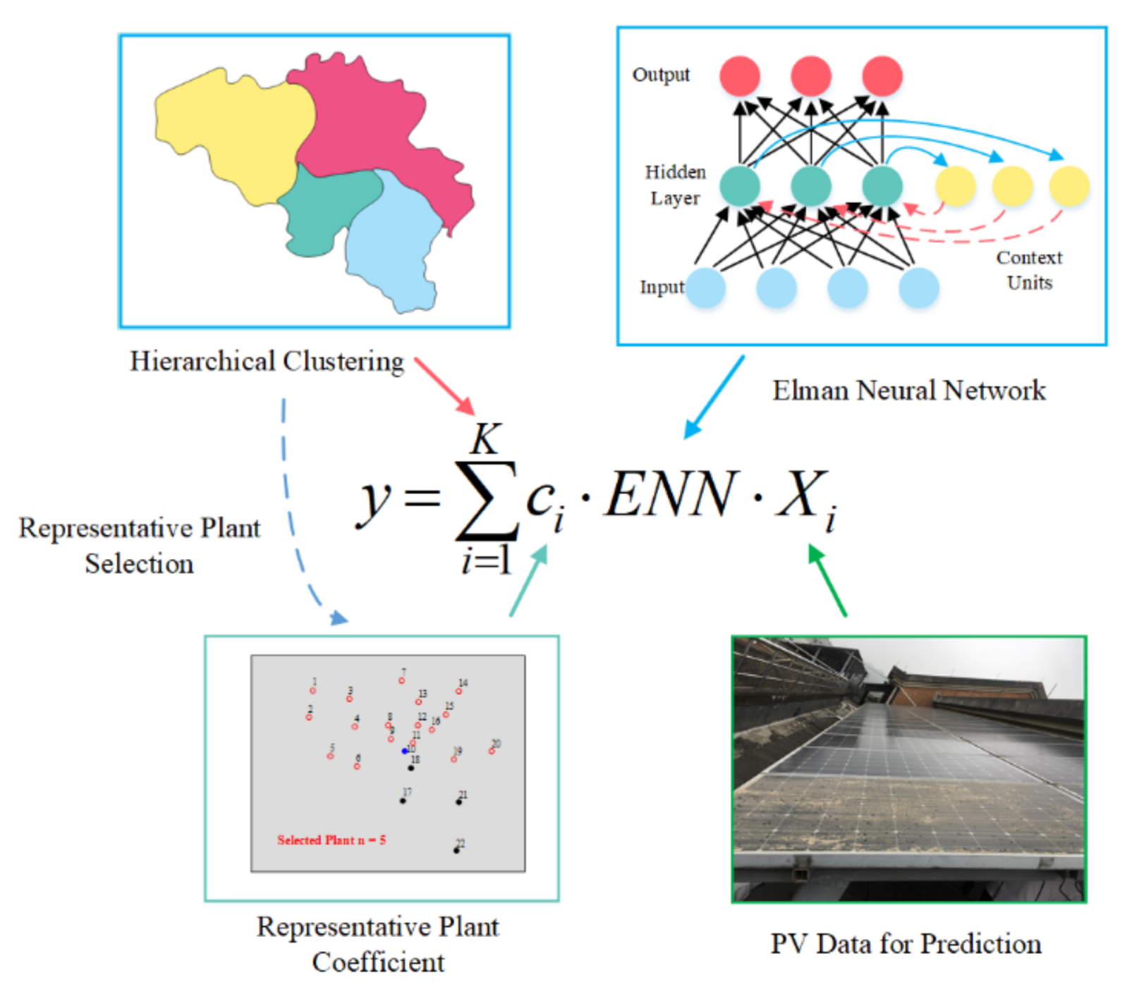
Elman neural network (ENN) is a local-feedback recursive neural network [37], which was proposed by Elman in 1990. Differing from other network like Convolutional Neural Network (CNN), the structure of an ENN layer is with connections that span through time. This means that the computations are done to an element of a sequence depending on the computations from previous elements of the same sequence. The construction of ENN is more suitable for time series as it assumes a causal association among the data [38,39]. The topology structure of ENN consists of the input layer, hidden layer, context layer and output layer, as shown in Figure 2. The input layer, hidden layer and output layer are connected like a feedforward network. In particular, the input layer units only work as an input signal transmission. The output units work as a linear weighting function. The hidden layer units work as linear or nonlinear transfer function. The context layer units, which work as one-step time delays, can transmit the previous information of the hidden layer to construct a feedback ring. As the context layer units have a storage effect on the hidden layer at a delayed time, ENN has dynamic memory and time-varying ability. Hence, ENN is widely used in time-series prediction [40,41]. As it discussed above, ENN is selected as the neural network type in this paper.

The state space equation of ENN is presented in Equation (16), where F() and G() represent the transfer function of the neurons in hidden layer and output layer, respectively. x(k) and x_c(k) represent the output units of the hidden layer and the context layer at time k, respectively. u(k − 1) represent the input layer units at time k − 1, y(k) represents the output layer units at time k. α₁ denotes the weight coefficients between the hidden layer and the context layer. α₂ denotes the weight coefficients between the hidden layer and the input layer. α₃ denotes the weight coefficients between the hidden layer and the output layer. b₁ and b₂ represent the threshold vectors of the hidden layer and output layer, respectively.

$$\begin{array}{l}x\left(k\right)=F\left[{\alpha }_1{x}_c\left(k\right)+{\alpha }_{2}u\left(k-1\right)+b_1\right]\\ x_c\left(k\right)=x\left(k-1\right)\\ y\left(k\right)=G\left[{\alpha }_{3}x\left(k\right)+b_2\right]\end{array}$$

(16)

3. Proposed Method

3.1. Representative Power Plant Selection Model

The selection of representative power plants is vital to guarantee the accuracy of sub-regional PV output prediction. Usually, the selection of representative power plants is based on the correlation between the power prediction accuracy of the single power plant and the regional power output. However, the high relevant power plants contain a large amount of redundant information in the region, which are not able to cover all the information of the sub-region. Therefore, this paper utilizes mutual information to characterize the correlation between the single power plants and the sub-region. Based on the mRMR criterion, the representative power plants are selected for the PV output power prediction. Figure 3 shows the specific procedure for the mRMR-based representative power plant selection model with the following steps:

(1)

Calculate the mutual information I(v, V) between the power output of each single power plant and the power output value of the sub-region, and calculate the mutual information I(v_i, v_j) between the single power plants in the sub-region;

(2)

When I(v, V) reaches the maximum, mark the data set S = {v}, F = F − {v};

(3)

Calculate the feature set F based on the incremental search algorithm, where the feature v satisfies Equation (14) and S = S ∪{v}, F = F − {v};

(4)

Determine whether the number of features in the subset reaches n. If so, output the subset S. Otherwise, repeat step (3) and continue the search until the number of features is n.

3.2. Proposed Algorithm

Combining the EOF decomposition, the mutual information and the upscaling prediction, a novel approach for the regional PV output prediction is proposed in this article. The main framework of the proposed method is presented in Figure 4. First, the historical data of PV power output is sorted for preprocessing, which include the abnormal data detection, the missing data fixing, and the blank data deleting. Second, the EOF decomposition for the historical PV output data is performed to obtain the vector matrix V. Then, the hierarchical clustering is performed to divide the power plant sub-region based on the obtained matrix. Meanwhile, by utilizing the mutual information, the correlation between the representative power plants and the sub-region is revealed. The mRMR criterion and the incremental search algorithm are adopted to search the optimal representative power plants. Afterwards, the upscaling prediction for each sub-region is performed based on the predicted PV output of the representative power plant. Finally, the predicted PV outputs of the sub-regions are added to obtain the PV output of the entire region. Additionally, the error analysis is performed to evaluate the proposed method.

To be specific, the PV output prediction of the representative power plants is realized by an Elman neural network. As referred to above, in the ENN model, the number of input neurons, hidden neurons and output neurons are set as 7, 10 and 1, respectively. The number of the hidden layer is set as 1. The transfer function and the training function are selected as Tansig and Traingdm, respectively. The learning rate is set as 0.05 and the maximum training epochs is set as 200. In order to verify the proposed method, the 70% PV power output data in time series are used as the training sample for ENN model. The remaining 30% data are used as the testing sample to validate the performance of ENN model. Then, the conception of the transform coefficient and the weighting factor is imported for the sub-regional output prediction. The transform coefficient is a function, which represents the PV output correlation between the representative power plants and the sub-region in average. Based on the mRMR algorithm, the optimal representative power plant is obtained. It reveals that the PV output characteristics of representative power plant is similar with the sub-region. Then, the ratio of the average PV output between the representative power plant and the sub-region is defined as the transform coefficient, which is shown in Equation (17).

$${\beta }_i=\frac{{\displaystyle {\sum }_{i=1}^n{P}_{Ri}}}{{\displaystyle {\sum }_{i=1}^n{P}_{Fi}}}$$

(17)

where n is the number of the available PV output data, and P_Ri and P_Fi are the i th actual output values of the sub-region and the representative power plant, respectively. For a sub-region, the number of the representative power plant is defined as l. The transform coefficient can be expressed by an l-order diagonal matrix H, as follows:

$$H=diag({\beta }_1,{\beta }_2,\cdot \cdot \cdot ,{\beta }_l)$$

(18)

Meanwhile, the weighting factor of the representative power plants represents the mutual information between the representative power plants and the sub-region. Since the representative power plants are selected, each plant correspondeds to a different weight for the sub-region. Then, the weight of each plant in the output prediction of the sub-region can be represented by its mutual information value. The weighting factor ω_j is calculated as follows:

$${\omega }_j=\frac{I(v_j,V)}{{\displaystyle {\sum }_{j=1}^{l}I(v_j,V)}}$$

(19)

where v_j is the PV output of the j th representative power plant, V is the average PV output of the sub-region, and I(v_j,V) is the degree of system uncertainty decrease. Then, the weighting factor of the representative power plants can constitute a weight vector $W={[{\omega }_1,{\omega }_2,\cdot \cdot \cdot ,{\omega }_k]}^T$. Combining the transform coefficient and the weighting factor, the PV output prediction of the sub-region can be calculated by Equation (20):

$$P_R=P_{F}HW$$

(20)

The entire regional PV output can be obtained by adding the PV output of all sub-regions. Moreover, the sub-region division is benefited in order to improve the accuracy of the entire regional PV output prediction and reduce the impact of the meteorological factors on PV output prediction under a wide area. Beyond that, the selection of representative power plants can greatly simplify the complexity of the prediction algorithm and improve the prediction speed. In order to visualize the implementation process, Figure 5 presents the main schematic diagram of the proposed method, where y represents the entire regional predicted PV power output, K represents the cluster numbers of sub-regions, c_i represents the representative PV plant coefficient of the corresponding sub-region, and X_i represents the training PV data for prediction.

4. Results and Discussion

4.1. Experimental Data Description

To verify the performance of the proposed method, the data collected from 22 PV power plants in Belgium are used as the experimental data [42]. The data recorded the output power between 05:30 and 21:45 from 16 May 2018 to 30 July 2018 with a time resolution of 15 min. There are 66 sets of data per day, including independent time data and 22 single farm power plant output powers. The installed capacity of the power plant is between 86.45 and 551.99 MW. Scaled according to the spatial locations, the geographic distribution of the PV power plants is shown in Figure 6, where the 22 PV single power plants are numbered from left to right.

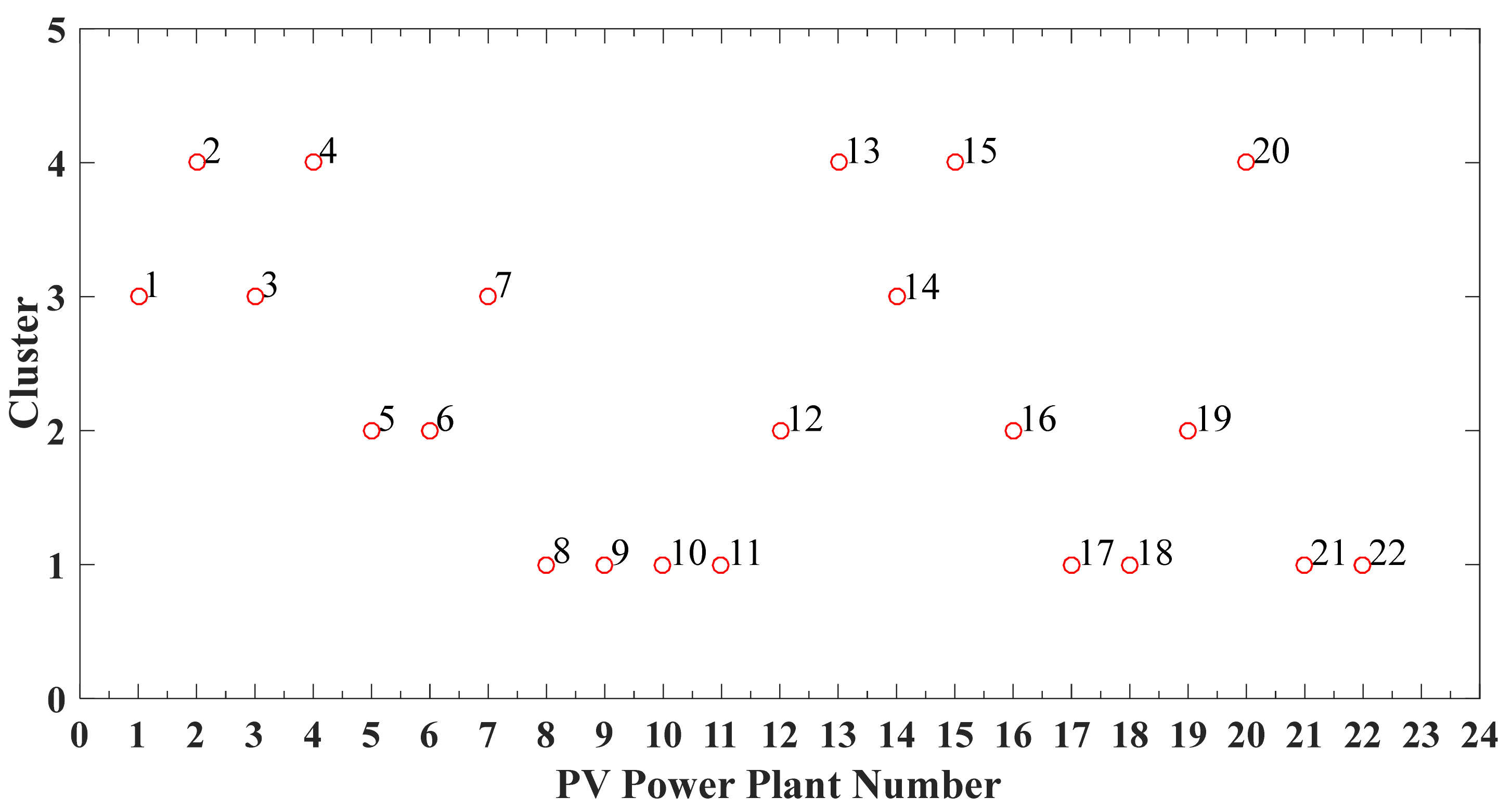
4.2. Sub-Region Division Analysis

Figure 7 presents the clustering process of the sub-region division. The abscissa is the serial number of the power plant, and the ordinate is the class the power plant belongs to. After EOF decomposition of the data of the 22 power plants, the spatial feature vectors obtained by the decomposition are used as reference values for the condensed hierarchical clustering to divide the region into sub-regions for all the power plants. Initially, each power plant is treated as a separate class. The similarity between each pair of power plants is calculated by Equation (6), and the two closest classes are combined into a new class. This process is continued until all power plants are clustered into one class, then the algorithm is terminated. To extensively consider the spatial range, the entire region is divided into four sub-regions, as shown in Figure 7 and Figure 8 below. Sub-region 1 contains five power plants, namely, No. 2, 4, 13, 15, and 20; sub-region 2 contains four power plants, namely, No. 1, 3, 7, and 14; sub-region 3 contains five power plants, namely, No. 5, 6, 12, 16, and 19; and sub-region 4 contains eight power plants, namely, No. 8, 9, 10, 11, 17, 18, 21, and 22.

After the sub-regions are obtained, the representative power plants in each sub-region are selected based on the mRMR criterion. The process of selecting the representative power plants in sub-region 4 is shown in Figure 9, where n is the set number of representative power plants. When n = 3, the algorithm selects power plants No. 17, 18, and 22 as the representative power plants. Since the spatial locations of power plants No. 8, 9,10 and 11 are close to the power plant No. 18, the mutual information is relatively large, so only plant No. 18 is selected as the representative. The selection of power plant No. 22 also fully demonstrates that the spatial distribution of the power plants selected by the model is maximized. When n = 5, plant No. 10 is added as a representative power plant. Power plants No. 10 and 18 have certain redundant information, demonstrating that the optimal representative power plant can be obtained using a reasonable value of n.

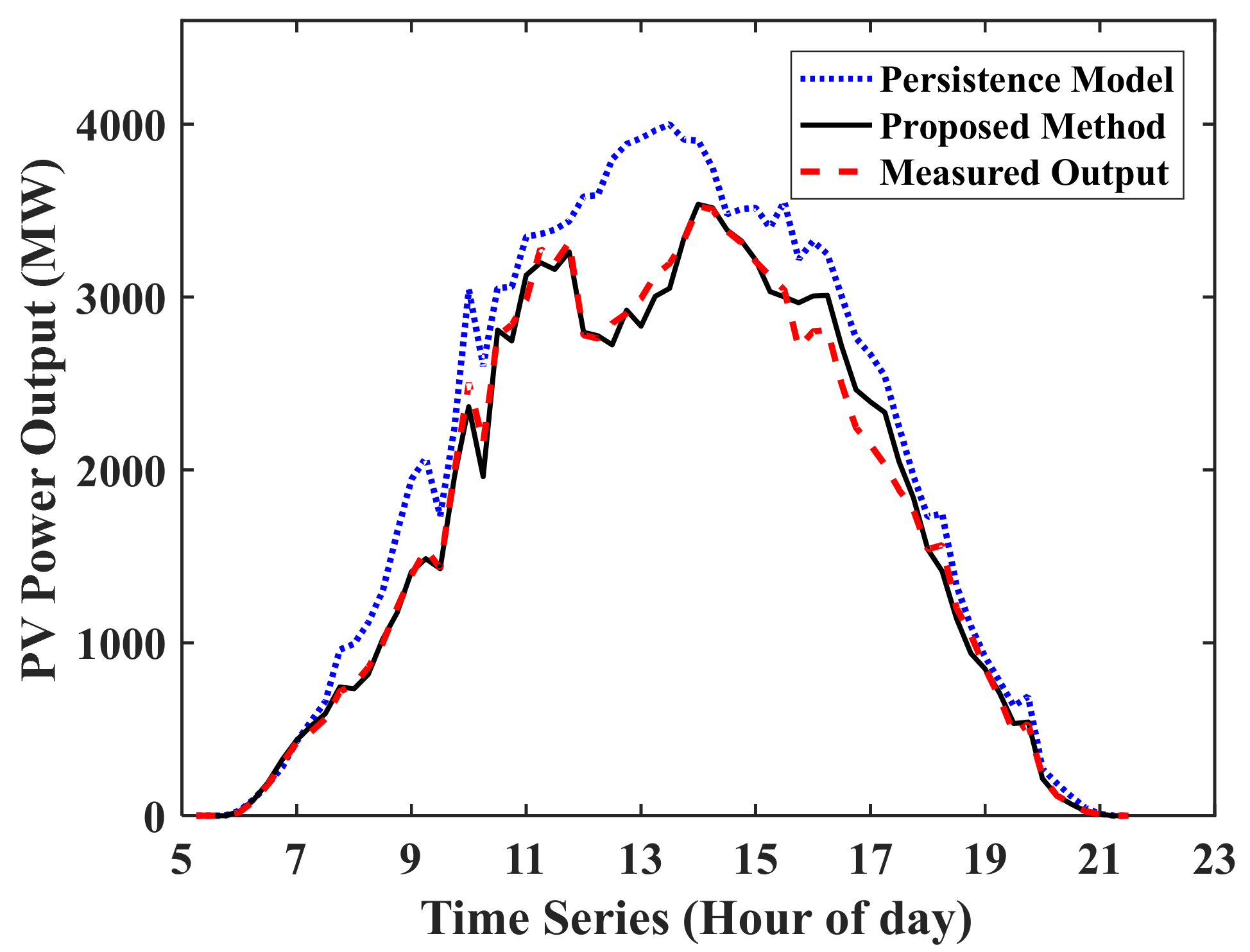
4.3. Regional PV Output Prediction

According to the above analysis, the entire region is divided into four sub-regions. Power plants No. 20 and 4 are selected as representative power plants for sub-region 1, power plants No. 7 and 3 are selected as representative power plants for sub-region 2, power plants No. 16 and 6 are selected as representative power plants for sub-region 3, and power plants No. 17, 18, 21 and 22 are selected as representative power plants for sub-region 4, since there are a greater number of power plants in this sub-region. The output transform coefficient and the output weighting factor of each representative power plant and sub-region are calculated by Equations (15) and (17), respectively, as shown in

Table 1. Transform coefficient and weighting factor of the representative power plants in each sub-region.

Value	Sub-Region 1		Sub-Region 2		Sub-Region 3		Sub-Region 4
Plant No.	20	4	7	3	16	6	17	18	22	21
Transform coefficient	6.697	4.469	3.903	3.995	5.035	4.236	5.997	5.147	8.154	6.803
Weighting factor	0.501	0.498	0.500	0.499	0.507	0.493	0.251	0.250	0.249	0.248

.

Observed from the transform coefficient and weighting factor in Table 1, the prediction value of the sub-region PV output is calculated by Equation (20). In particular, the experimental data from the 22 power plants throughout Belgium on 1 August were selected to verify the algorithm. The predicted and actual values of the sub-region 1, 2, 3 and 4 are shown in Figure 10, respectively. Then, the predicted values of the four sub-regions are added to obtain the predicted value of the full-region PV output, as shown in Figure 10. Although some parts of the prediction and the actual output value of the sub-regions have large errors in Figure 10, the error of the entire regional prediction output in Figure 11 is much smaller than the value in each sub-region after integration of the four regions. This is because in the time interval from 16:00 to 19:00, the predicted output values of sub-region 2 in Figure 10b and sub-region 3 in Figure 10c are larger than the actual measured values, while the predicted output values of sub-region 1 in Figure 10a and sub-region 4 in Figure 10d are smaller than the actual values. The power output of the entire region in Figure 11 is obtained by superimposing the value of each sub-region to reduce the prediction error, causing the predicted values of the entire region to be closer to the actual output values.

Interestingly, observed from Figure 11, when the PV output is relatively flat, the prediction results are very ideal. However, when the output fluctuates greatly, the prediction result also has a certain fluctuation, and the prediction accuracy is not good. The prediction curve by this algorithm can track the actual output variation curve of the region; the predicted value deviates from the actual curve only when the output of individual power plants fluctuates greatly.

Although some parts of the prediction curve and the actual output curve of the sub-regions have large errors, the error of the entire regional prediction curve after integration of the four regions is much smaller than that of the sub-regions. This is because in the time interval of 40–50, the predicted output values of sub-regions 2 and 4 are larger than the actual values, while the predicted output values of sub-regions 1 and 3 are smaller than the actual values. The PV output value of the entire region is obtained by superimposing the value of each sub-region to reduce the prediction error, causing the predicted values of the entire region to be closer to the actual output values.

Additionally, the normalized mean absolute error (nMAE) and the normalized root mean square error (nRMSE) are imported to present the prediction errors. As shown in Equation (21), P_pred represents the predicted power of a PV system, P_meas represents the measured power of a PV system, and P_nom represents the nominal power of the PV system.

$$\begin{array}{l}nMAE=\frac{1}{N}{\displaystyle \sum _{t=1}^N\frac{\left|P_{pred}-P_{meas}\right|}{P_{nom}}}\times 100\%\\ nRMSE=\sqrt{\frac{1}{N}{{\displaystyle \sum _{t=1}^N\left(\frac{P_{pred}-P_{meas}}{P_{nom}}\right)}}^2}\times 100\%\end{array}$$

(21)

Table 2. Prediction error comparison of sub-regions and the entire region.

Error Analysis	Sub-Region 1	Sub-Region 2	Sub-Region 3	Sub-Region 4	Entire Region
Mean absolute error (MAE)	5.13%	6.83%	6.62%	5.73%	4.69%
Root mean square error (RMSE)	6.10%	7.58%	7.19%	6.50%	5.67%

lists the prediction errors of each sub-region and the entire region. To eliminate the prediction error of the representative power plants, it is ideally assumed that the prediction error of each single farm power plant is 0; that is, the prediction accuracies of different power plants are the same. Obviously, due to the smoothing effect, the prediction errors of different power plant outputs cancel each other out, which decreases the overall error and hence causing the prediction error of the entire region to be smaller than that of single farms.

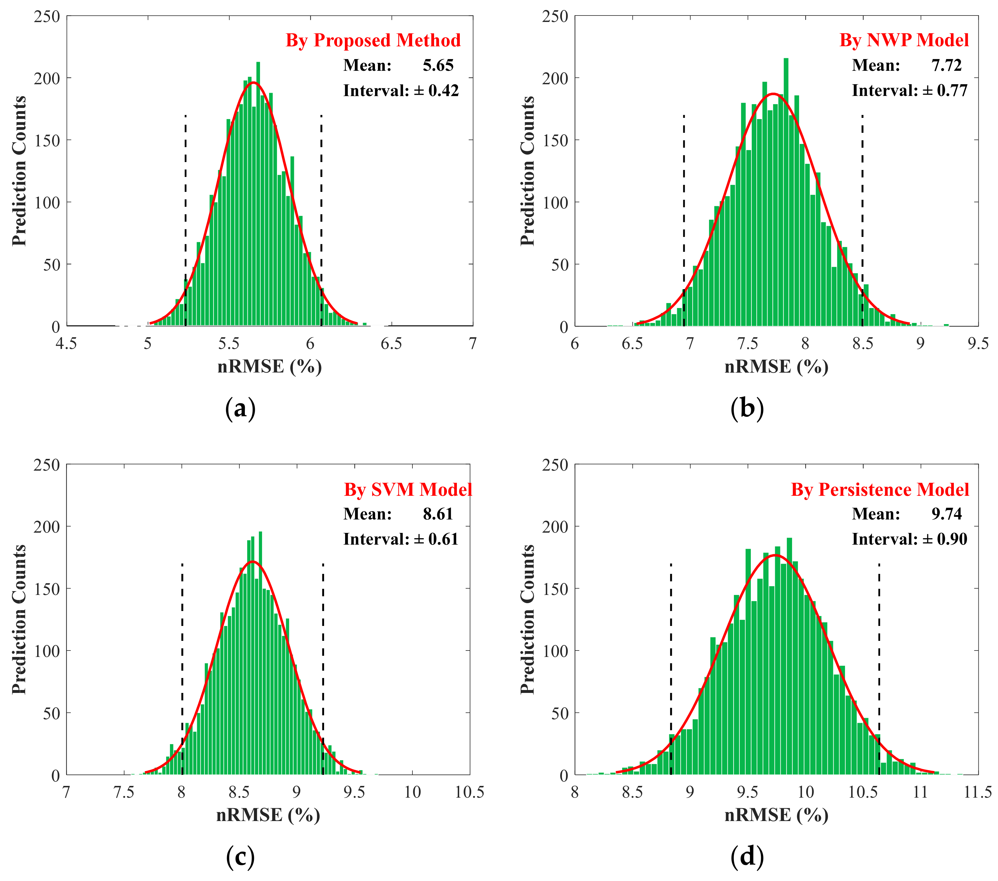
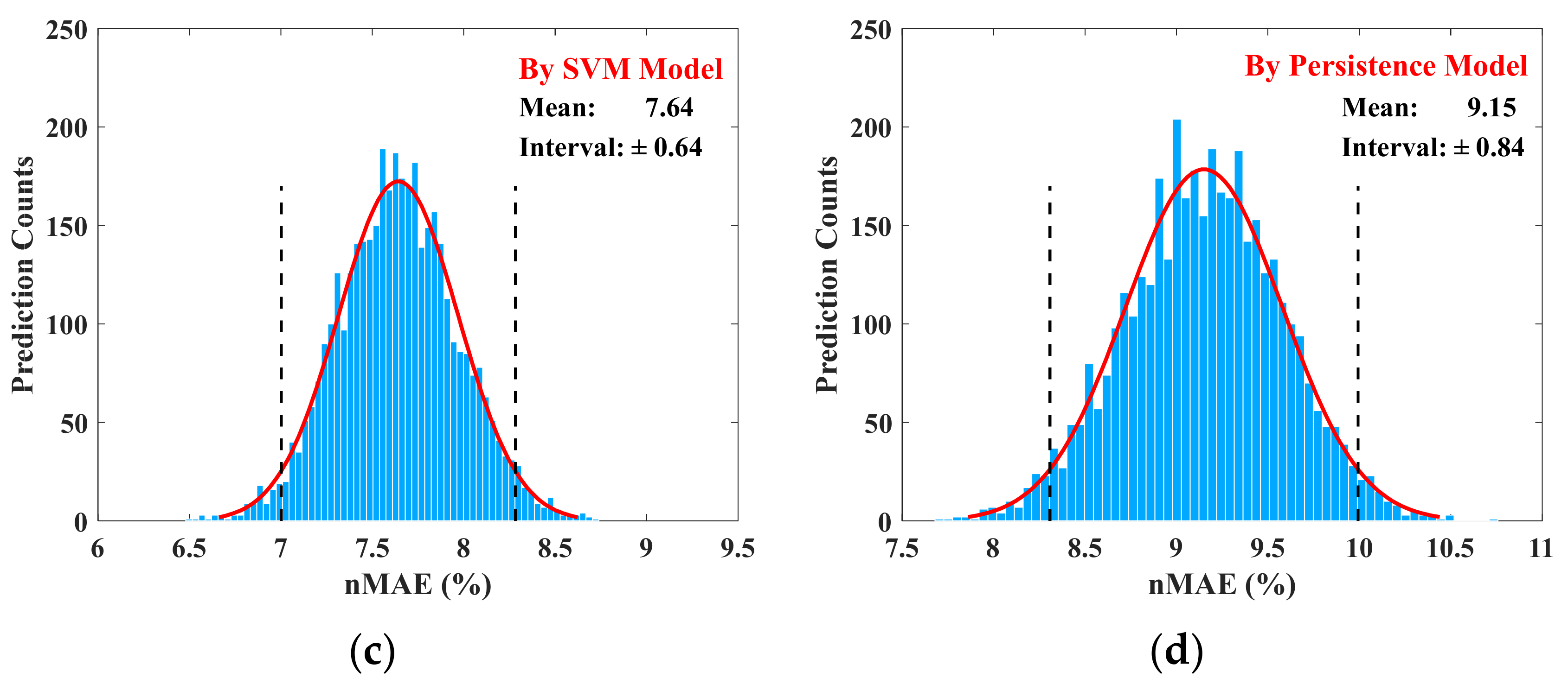
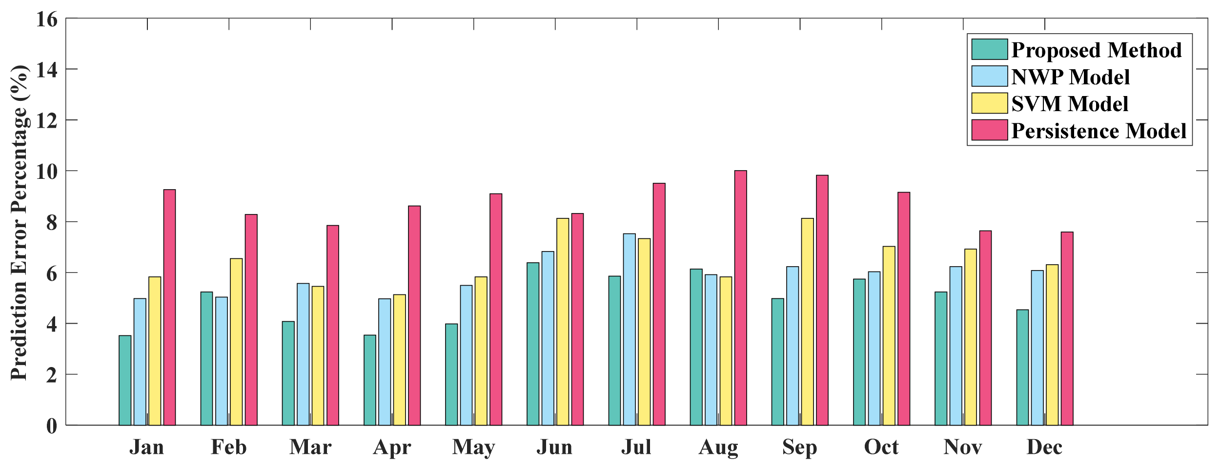
4.4. Performance Analysis

To further investigate the effectiveness of the proposed method, three methods are imported in the regional PV power prediction, which are the persistence model, NWP (Numerical weather prediction) model, and SVM model. The persistence model is a simple but widely-used method to forecast the PV power output in real application. The detail of the persistence model is presented in [43]. The NWP model converts the irradiance to the regional power based on the input parameters of the PV panel. The prediction power of each cluster is first predicted by using the three NWP forecasts. Then, the prediction power of the representative plant is obtained and optimized by adding an efficiency and bias correction [44]. Support vector machine (SVM) is a common technique of machine learning to regress the feature data into an output number. In order to make a fair comparison, the SVM method will follow the same data preprocessing in this paper, including bad data clean, historical data reconstruction. The SVM model is firstly trained to build the relationship between the data features and the real PV power output. Then, the application of the SVM is conducted for the PV power forecasting. The detail of the SVM model for regional PV power prediction is presented in [45].

Since the persistence model is regarded as the reference, any other prediction method should perform better than the persistence method. For instance, the prediction curves of the proposed method and the persistence method are compared with the actual output power curve in Figure 12. It can be seen that when the actual output is small, the two prediction algorithms have only slight errors. As the actual output power increases, the prediction value of the traditional prediction method is significantly larger, while the prediction value by the proposed algorithm fluctuates in a small range around the actual output power.

It can be seen from the analysis of the PV output fluctuation that when the PV output value is large, the fluctuation is large. However, with the persistence method, the first k power plants with the most correlation are selected as the representative power plants, which include more redundant information. After the regional prediction is added up, the redundant information is superimposed, causing large deviations to appear, as demonstrated, to a certain extent, by the fluctuation of the predicted value by the persistence method with the actual output. For example, in the time interval of 25 to 40, the persistence method prediction algorithm leads to a large error.

Figure 13 presents the prediction result of PV output versus the measured value by utilizing the proposed method and other methods. In order to show a better comparison, the power value is normalized from 0 to 1. The red solid line y = x provides a reference when prediction value is equal to the measure value. The blue points represent the prediction value and the corresponding real power value in the same time. The dispersion degree of the blue points around the red line reflects the error between measured power and prediction power. The more intensively the blue points aggregate to the red lines, the less forecasting error of the corresponding model shows. Observed from Figure 13d, the blue points of the persistence method reveal the sparse distribution from the red line. Meanwhile, the blue points of the NWP method and SVM method concentrated more intensively to the red line compared with the persistence method in Figure 13b,c, respectively. The results of the proposed method in Figure 13a show clear aggregating characteristics to the reference red line.

As shown in Figure 13, the distribution of the measured power versus prediction power points reveals an intuitive comparison between different prediction methods. However, the comparison of performance analysis in Figure 13 seems intuitive, which in not reliable in quantitative evaluation. Therefore, the error histograms of the regional PV power estimation are described for both nMAE and nRMSE in Figure 14 and Figure 15, respectively. Observed from the histograms, the prediction error exhibits an approximately normal distribution. The mean value and the 95% confidence interval are also marked. Since the regional PV prediction is independent of the random condition, the prediction error is also random in order to show a normal distribution. Hence, the normally distributed result presented in Figure 14 and Figure 15 indicated that the forecasting result was reliable. Moreover, the average nRMSE for the proposed method, the NWP model, SVM model, and persistence model were 5.65, 7.72, 8.61, and 9.74, respectively. The 95% confidence intervals of these nRMSE were 5.65 ± 0.42, 7.72 ± 0.77, 8.61 ± 0.61, and 9.74 ± 0.90, respectively. Meanwhile, the average nMAE for the proposed method, NWP model, SVM model, and persistence model were 4.68, 6.45, 7.64, and 9.15, respectively. The 5% confidence intervals of these nMAE were 4.68 ± 0.49, 6.45 ± 0.72, 7.64 ± 0.75, and 9.15 ± 0.84, respectively. Thus, both error analyses could represent the performance of four prediction methods. Based on the performance analysis, it can be observed that the proposed method leads to a lower average nRMSE and nMAE than the other prediction methods. Additionally, we noted that the 95% confidence interval range for the proposed method was approximately 30% less than for the NWP model and SVM model.

Figure 16 presents a comparative analysis between the proposed method, NWP model, SVM model, and persistence model. Both the average and the quartile of the nRMSE and nMAE are presented and marked by using the error statistics method. The forecast performance is quite similar for the NWP model and the SVM model. Specifically, for the proposed method, the average of the nMAE is reduced by 4.68% and the average of the nRMSE is reduced by 5.65%. Meanwhile, the average of the nRMSE predicted by the NWP model, the SVM model and the persistence model is 7.72%, 8.61% and 9.71% respectively. Meanwhile, the average nMAE of the predicted by the NWP model, the SVM model and the persistence model is 6.46%, 7.64% and 8.62% respectively. Moreover, the upper and lower quartiles of the nRMSE and nMAE also show the robust result. For instance, the nRMSE intervals of the upper and lower quartiles calculated by the proposed method, the NWP model, the SVM model, and the persistence model are 0.43%, 0.79%, 0.64%, and 0.92%, respectively. The nNAE intervals of the upper and lower quartiles calculated by the proposed method, the NWP model, the SVM model, and the persistence model is 0.50%, 0.72%, 0.68%, and 0.88%, respectively. Based on what discussed above, the experiment results verified the proposed method has a better forecasting performance than the other models.

The advantage of the sub-region division algorithm based on EOF and hierarchical clustering fully considers the spatiotemporal characteristics of PV output. In this method, it can effectively describe the PV output correlation based on the cosine similarity. Meanwhile, it is able to depict the PV data correlation of the profiles by reducing the sensitivity of the absolute numerical values. Additionally, the representative power plant selection algorithm based on the mRMR criterion makes the selected power plants sufficiently representative and filters the redundant information. In summary, the sub-region division model and the representative power plant selection model achieve good forecast accuracy for regional PV prediction. Specifically, this proposed method is suitable for situations where the monitoring system is not available for every single PV power plant in a region or the PV power generation is not measured regionally.

To further verify the environmental variations, Figure 17 presents the monthly nMAE calculated with the proposed method, the NWP model, the SVM model and the persistence model from 1 January 2018 to 31 December 2018. Observed from the monthly prediction results, the annual average nMAE predicted by the proposed method, the NWP model, the SVM model and the persistence model is 4.62%, 6.35%, 6.75%, and 8.87% respectively. All the prediction results show fluctuation with seasonal variations. Overall, it was found that the proposed method still shows the better performance during most times. However, a few exceptions did occur in February and August. Meanwhile, the persistence model still presented a particularly poor performance during the year. The experimental results verify that: (1) the proposed method shows robust performance with seasonal variations; (2) our proposed method shows better predicted accuracy compared with the other prediction method by using different datasets.

5. Conclusions

This paper presents a new prediction method for the entire region’s PV power generation, which aims to provide a power dispatching strategy for a wide region. Considering the incomplete power data for some PV plants, a sub-region division model is proposed based on EOF decomposition and hierarchical clustering, which is fully represented by the time–space characteristics of the PV power. Subsequently, mutual information is adopted to reveal the correlation between the power plants and the sub-region. On the basis of the sub-region division, the representative power plant selection model is proposed by utilizing the mRMR criterion. In particular, this model not only considers the correlation between the power plants and the sub-region, but also reduces redundant information for the selection of the representative PV plants. The PV output prediction for each sub-region is achieved by utilizing the Elman neural network. Finally, the predicted values of the four sub-regions are added to obtain the predicted value of the full-region PV output. Several experiments were performed and analyzed to investigate the validity of the proposed method. The conclusions of this research are summarized as follows:

• The sub-region division model based on the EOF decomposition and hierarchical clustering has the ability to describe the time–space characteristics of the PV power plants, which is more reasonable compared with the sub-region division method only by geographical locations.
• The representative power plant selection is beneficial and vital for the power output prediction of the regional PV plants. By utilizing the mRMR criterion, both accuracy and the computational efficiency will be improved. Additionally, faced with the lack of power data for some PV plants, the advantage of the representative selection model will surpass other PV prediction methods.
• The proposed prediction algorithm can mitigate the adverse impact of fluctuating PV power output. Particularly, the prediction errors are small regardless of whether the regional PV output ranges are flat or greatly fluctuating. The results from an annual case study show that, compared with the NWP model, the SVM model and the persistence model, the proposed prediction method reduces the nMAE by 4.62%, thereby effectively improving the prediction accuracy.

References

1. Marinelli, M.; Maule, P.; Hahmann, A.N.; Gehrke, O.; Norgard, P.B.; Cutululis, N.A. Wind and photovoltaic large-scale regional models for hourly production evaluation. IEEE Trans. Sustain. Energy 2015, 6, 916–923. [Google Scholar] [CrossRef]
2. Beranek, V.; Olsan, T.; Libra, M.; Poulek, V.; Sedlacek, J.; Dang, M.Q.; Tyukhov, I.I. New monitoring system for photovoltaic power plants’ management. Energies 2018, 1, 2495. [Google Scholar] [CrossRef]
3. Libra, M.; Beranek, V.; Sedlacek, J.; Poulek, V.; Tyukhov, I.I. Roof photovoltaic power plant operation during the solar eclipse. Sol. Energy 2016, 140, 109–112. [Google Scholar] [CrossRef]
4. Fu, L.; Wei, Y.D.; Fang, S.; Zhou, X.J.; Lou, J.Q. Condition monitoring for roller bearings of wind turbines based on health evaluation under variable operating states. Energies 2017, 10, 1564. [Google Scholar] [CrossRef]
5. Fu, L.; Wei, Y.D.; Fang, S.; Tian, G.; Zhou, X.J. A wind energy generation replication method with wind shear and tower shadow effects. Adv. Mech. Eng. 2018, 10, 3. [Google Scholar] [CrossRef]
6. Meral, M.E.; Dincer, F. A review of the factors affecting operation and efficiency of photovoltaic based electricity generation systems. Renew. Sust. Energ. Rev. 2011, 5, 2176–2184. [Google Scholar] [CrossRef]
7. Reikard, G. Predicting solar radiation at high resolutions: A comparison of time series forecasts. Sol. Energy. 2009, 83, 342–349. [Google Scholar] [CrossRef]
8. Bae, K.Y.; Jang, H.S.; Sung, D.K. Hourly solar irradiance prediction based on support vector machine and its error analysis. IEEE Trans. Power Syst. 2019, 32, 935–945. [Google Scholar] [CrossRef]
9. Rodriguez, F.; Fleetwood, A.; Galarza, A.; Fontan, L. Predicting solar energy generation through artificial neural networks using weather forecasts for microgrid control. Renew. Energy 2018, 126, 855–864. [Google Scholar] [CrossRef]
10. Lin, P.J.; Peng, Z.N.; Lai, Y.F.; Cheng, S.Y.; Chen, Z.C.; Wu, L.J. Short-term power prediction for photovoltaic power plants using a hybrid improved Kmeans-GRA-Elman model based on multivariate meteorological factors and historical power datasets. Energy Conv. Manag. 2018, 177, 704–717. [Google Scholar] [CrossRef]
11. Lamsal, D.; Sreeram, V.; Mishra, Y.; Kumar, D. Achieving a minimum power fluctuation rate in wind and photovoltaic output power using discrete Kalman filter based on weighted average approach. IET Renew. Power Gener. 2018, 12, 633–638. [Google Scholar] [CrossRef]
12. Chow, C.W.; Urquhart, B.; Lave, M.; Dominguez, A.; Kleissl, J.; Shields, J.; Washom, B. Intra-hour forecasting with a total sky imager at the UC San Diego solar energy testbed. Sol. Energy 2011, 85, 2881–2893. [Google Scholar] [CrossRef] [Green Version]
13. Zeng, J.W.; Qiao, W. Short-term solar power prediction using a support vector machine. Renew. Energy. 2013, 52, 118–127. [Google Scholar] [CrossRef]
14. Cao, J.C.; Lin, X.C. Study of hourly and daily solar irradiation forecast using diagonal recurrent wavelet neural networks. Energy Conv. Manag. 2008, 49, 1396–1406. [Google Scholar] [CrossRef]
15. Demirhan, H.; Renwick, Z. Missing value imputation for short to mid-term horizontal solar irradiance data. Appl. Energy. 2018, 225, 998–1012. [Google Scholar] [CrossRef]
16. Lorenz, E.; Hurka, J.; Heinemann, D.; Beyer, H.G. Irradiance forecasting for the power prediction of grid-connected photovoltaic systems. IEEE J. Sel. Top. Appl. Earth Observ. Remote Sens. 2009, 2, 2–10. [Google Scholar] [CrossRef]
17. Lipperheide, M.; Bosch, J.L.; Kleissl, J. Embedded nowcasting method using cloud speed persistence for a photovoltaic power plant. Sol. Energy 2015, 112, 232–238. [Google Scholar] [CrossRef]
18. Lonij, V.P.A.; Brooks, A.E.; Cronin, A.D.; Leuthold, M.; Koch, K. Intra-hour forecasts of solar power production using measurements from a network of irradiance sensors. Sol. Energy 2013, 97, 58–66. [Google Scholar] [CrossRef]
19. Pierro, M.; De Felice, M.; Maggioni, E.; Moser, D.; Perotto, A.; Spade, F.; Cornaro, C. Data-driven upscaling methods for regional photovoltaic power estimation and forecast using satellite and numerical weather prediction data. Sol. Energy 2017, 158, 1026–1038. [Google Scholar] [CrossRef]
20. Fonseca, J.G.D.; Oozeki, T.; Ohtake, H.; Takashima, T.; Ogimoto, K. Regional forecasts of photovoltaic power generation according to different data availability scenarios: A study of four methods. Prog. Photovoltaics 2015, 23, 1203–1218. [Google Scholar] [CrossRef]
21. Saint-Drenan, Y.M.; Good, G.H.; Braun, M.; Freisinger, T. Analysis of the uncertainty in the estimates of regional PV power generation evaluated with the upscaling method. Sol. Energy 2016, 135, 536–550. [Google Scholar] [CrossRef] [Green Version]
22. Malvoni, M.; De Giorgi, M.G.; Congedo, P.M. Photovoltaic forecast based on hybrid PCA-LSSVM using dimensionality reducted data. Neurocomputing 2016, 211, 72–83. [Google Scholar] [CrossRef]
23. Fonseca, J.G.D.; Oozeki, T.; Takashima, T.; Koshimizu, G.; Uchida, Y.; Ogimoto, K. Use of support vector regression and numerically predicted cloudiness to forecast power output of a photovoltaic power plant in Kitakyushu, Japan. Prog. Photovoltaics 2012, 20, 874–882. [Google Scholar] [CrossRef]
24. Saint-Drenan, Y.M.; Good, G.H.; Braun, M. A probabilistic approach to the estimation of regional photovoltaic power production. Sol. Energy 2017, 147, 257–276. [Google Scholar] [CrossRef] [Green Version]
25. Shaker, H.; Zareipour, H.; Wood, D. Impacts of large-scale wind and solar power integration on California’s net electrical load. Renew. Sust. Energ. Rev. 2016, 58, 761–774. [Google Scholar] [CrossRef]
26. Shivashankar, S.; Mekhilef, S.; Mokhlis, H.; Karimi, M. Mitigating methods of power fluctuation of photovoltaic (PV) sources—A review. Renew. Sust. Energ. Rev. 2016, 59, 1170–1184. [Google Scholar] [CrossRef]
27. Zhang, J.; Hodge, B.M.; Lu, S.Y.; Hamann, H.F.; Lehman, B.; Simmons, J.; Campos, E.; Banunarayanan, V.; Black, J.; Tedesco, J. Baseline and target values for regional and point PV power forecasts: Toward improved solar forecasting. Sol. Energy 2015, 122, 804–819. [Google Scholar] [CrossRef] [Green Version]
28. Zhu, T.; Qu, Z.; Xu, H.; Zhang, J.; Shao, Z.; Chen, Y.; Prabhakar, S.; Yang, J. RiskCog: Unobtrusive real-time user authentication on mobile devices in the wild. IEEE Trans. Mob. Comput. 2019. [Google Scholar] [CrossRef]
29. Fu, L.; Zhu, T.; Zhu, K.; Yang, Y.Y. Condition monitoring for the roller bearings of wind turbines under variable working conditions based on the fisher score and permutation entropy. Energies 2019, 12, 804–819. [Google Scholar] [CrossRef]
30. Farzaneh, S.; Forootan, E. Reconstructing regional ionospheric electron density: A combined spherical slepian function and empirical orthogonal function approach. Surv. Geophys. 2018, 39, 289–309. [Google Scholar] [CrossRef]
31. Aliahmadipour, L.; Eslami, E. GHFHC: Generalized hesitant fuzzy hierarchical clustering algorithm. Int. J. Intell. Syst. 2016, 31, 855–871. [Google Scholar] [CrossRef]
32. Tellaroli, P.; Bazzi, M.; Donato, M.; Brazzale, A.R.; Draghici, S. Cross-Clustering: A partial clustering algorithm with automatic estimation of the number of clusters. PLoS ONE 2016, 11, 3. [Google Scholar] [CrossRef] [PubMed]
33. Ge, Y.; Avitabile, V.; Heuvelink, G.B.M.; Wang, J.H.; Herold, M. Fusion of pan-tropical biomass maps using weighted averaging and regional calibration data. Int. J. Appl. Earth Obs. Geoinf. 2014, 31, 13–24. [Google Scholar] [CrossRef]
34. Herman, G.; Zhang, B.; Wang, Y.; Ye, G.; Chen, F. Mutual information-based method for selecting informative feature sets. Pattern Recognit. 2014, 46, 3315–3327. [Google Scholar] [CrossRef]
35. Paninski, L. Estimation of entropy and mutual information. Neural Comput. 2003, 15, 3315–3327. [Google Scholar] [CrossRef]
36. Peng, H.C.; Long, F.H.; Ding, C. Feature selection based on mutual information: Criteria of max-dependency, max-relevance, and min-redundancy. IEEE Trans. Pattern Anal. Mach. Intell. 2005, 27, 1226–1238. [Google Scholar] [CrossRef] [PubMed]
37. Lin, W.M.; Hong, C.M.; Chen, C.H. Neural-network-based mppt control of a stand-alone hybrid power generation system. IEEE Trans. Power Electron. 2011, 26, 3571–3581. [Google Scholar] [CrossRef]
38. Dong, Q.C.; Feng, J.Q. Outlier detection and disparity refinement in stereo matching. J. Vis. Commun. Image Represent. 2019, 60, 380–390. [Google Scholar] [CrossRef]
39. Dong, Q.C.; Feng, J.Q. Adaptive disparity computation using local and non-local cost aggregations. Multimed. Tools Appl. 2018, 77, 31647–31663. [Google Scholar] [CrossRef]
40. Yang, L.; Wang, F.; Zhang, J.J.; Ren, W.H. Remaining useful life prediction of ultrasonic motor based on Elman neural network with improved particle swarm optimization. Measurement 2019, 143, 27–38. [Google Scholar] [CrossRef]
41. Lan, H.; Zhang, C.; Hong, Y.Y.; He, Y.; Wen, S.L. Day-ahead spatiotemporal solar irradiation forecasting using frequency based hybrid principal component analysis and neural network. Appl. Energy. 2019, 247, 389–402. [Google Scholar] [CrossRef]
42. De Schepper, E.; Van Passel, S.; Lizin, S.; Achten, W.M.J. Cost-efficient emission abatement of energy and transportation technologies: Mitigation costs and policy impacts for Belgium. Clean Technol. Environ. Policy 2014, 16, 1107–1118. [Google Scholar] [CrossRef]
43. Pierro, M.; Bucci, F.; De Felice, M.; Maggioni, E.; Moser, D.; Perotto, A.; Spada, F.; Cornaro, C. Multi-Model ensemble for day ahead prediction of photovoltaic power generation. Sol. Energy 2016, 134, 132–146. [Google Scholar] [CrossRef]
44. Mittermaier, M.P.; Bullock, R. Using MODE to explore the spatial and temporal characteristics of cloud cover forecasts from high-resolution NWP models. Meteorol. Appl. 2013, 20, 187–196. [Google Scholar] [CrossRef] [Green Version]
45. Bacher, P.; Madsen, H.; Nielsen, H.A. Online short-term solar power forecasting. Sol. Energy 2009, 83, 772–1783. [Google Scholar] [CrossRef]
Figure 1. Flow chart of the sub-region division model.
Energies 12 03817 g001
Figure 2. Topology construction of the Elman neural network.
Energies 12 03817 g002
Figure 3. Flow chart for the representative power plant selection model.
Energies 12 03817 g003
Figure 4. Main framework of the proposed method.
Energies 12 03817 g004
Figure 5. Main schematic diagram of the proposed method.
Energies 12 03817 g005
Figure 6. Schematic diagram of geographical distribution of photovoltaic (PV) power plants in Belgium.
Energies 12 03817 g006
Figure 7. Cluster process of sub-region division.
Energies 12 03817 g007
Figure 8. Cluster result of sub-region division.
Energies 12 03817 g008
Figure 9. Selection process of the representative power plant in sub-region 4. (a) when the selected number is 2; (b) when the selected number is 3; (c) when the selected number is 4; (d) when the selected number is 5.
Energies 12 03817 g009
Figure 10. Sub-region PV output prediction results. (a) PV power prediction of sub-region 1; (b) PV power prediction of sub-region 2; (c) PV power prediction of sub-region 3; (d) PV power prediction of sub-region 4.
Energies 12 03817 g010
Figure 11. Regional output prediction.
Energies 12 03817 g011
Figure 12. Regional output predictions compared with proposed method and persistence model.
Energies 12 03817 g012
Figure 13. The real measured power versus prediction power on regional output: (a) using the proposed method; (b) using the NWP (Numerical weather prediction) model; (c) using the support vector machine (SVM) model; (d) using the persistence model.
Energies 12 03817 g013
Figure 14. Histogram comparison of the forecast nRMSE: (a) using the proposed method; (b) using the NWP model; (c) using the SVM model; (d) using the persistence model.
Energies 12 03817 g014
Figure 15. Histogram comparison of the forecast nMAE: (a) using the proposed method; (b) using the NWP model; (c) using the SVM model; (d) using the persistence model.
Energies 12 03817 g015aEnergies 12 03817 g015b
Figure 16. Error comparison of each regional forecast method.
Energies 12 03817 g016
Figure 17. Monthly nMAE percentage comparison of each regional forecast method.
Energies 12 03817 g017