Deep Ensemble Learning Model for Short-Term Load Forecasting within Active Learning Framework

Abstract

Short term load forecasting (STLF) is one of the basic techniques for economic operation of the power grid. Electrical load consumption can be affected by both internal and external factors so that it is hard to forecast accurately due to the random influencing factors such as weather. Besides complicated and numerous internal patterns, electrical load shows obvious yearly, seasonal, and weekly quasi-periodicity. Traditional regression-based models and shallow neural network models cannot accurately learn the complicated inner patterns of the electrical load. Long short-term memory (LSTM) model features a strong learning capacity to capture the time dependence of the time series and presents the state-of-the-art performance. However, as the time span increases, LSTM becomes much harder to train because it cannot completely avoid the vanishing gradient problem in recurrent neural networks. Then, LSTM models cannot capture the dependence over large time span which is of potency to enhance STLF. Moreover, electrical loads feature data imbalance where some load patterns in high/low temperature zones are more complicated but occur much less often than those in mild temperature zones, which severely degrades the LSTM-based STLF algorithms. To fully exploit the information beneath the high correlation of load segments over large time spans and combat the data imbalance, a deep ensemble learning model within active learning framework is proposed, which consists of a selector and a predictor. The selector actively selects several key load segments with the most similar pattern as the current one to train the predictor, and the predictor is an ensemble learning-based deep learning machine integrating LSTM and multi-layer preceptor (MLP). The LSTM is capable of capturing the short-term dependence of the electrical load, and the MLP integrates both the key history load segments and the outcome of LSTM for better forecasting. The proposed model was evaluated over an open dataset, and the results verify its advantage over the existing STLF models.

1. Introduction

With the rapid development of the economy, the demand for electricity increases rapidly. To meet the electricity demand, renewable energies and distributed electricity generation have emerged as an important part of electrical energy. The randomness of these kinds of energies may bring a impulse to the power grid, thus the thermal power generation requires accurate planning according to the renewable energy generation and social electricity consumption to balance the power generation and consumption. The high randomness of renewable energy generation calls for a more flexible and intelligent scheduling technology to solve the problem [1]. At the same time, the rapid increase in both type and quantity of the electricity consumption leads to drastic variation in the electrical load, which worsens the regional load imbalance severely. As an important functionality of the energy management system, accurate electrical load forecasting plays an important role for efficient dispatching and enhanced grid quality [2].

As a classical time series forecasting problem, short-term load forecasting (STLF) has attracted much attention from both academia and industry since the 1950s, and various methods have been proposed ever since [3,4,5,6,7,8,9,10,11,12,13]. The existing algorithms can be roughly classified into two categories: statistical methods and machine learning methods. Statistical methods include similar day method and regressive-type methods. The similar day method [3] searches for the historical electrical load segments with the same attribute values (e.g., climate, day of the week, and date) as the current one to be predicted, and then, makes a prediction via weighting the selected historical load segments. Although simple and effective, it depends on the correct choice of affecting factors, and it will degrade severely when some important affecting factors are missing. Regression-type methods analyze the correlation between variables via statistics. When applied to electricity load prediction, electricity loads are regarded as relevant data, while external factors such as temperature and date are copied as independent variables. Then, regression methods model the correlation between loads and external variables [4,5]. Regression-type models, including Autoregressive moving average (ARMA) [6] and many other enhanced models [7,8], although taking the non-stationarity of time series and the influence of external factors into consideration, are not designed for the task with typical non-stationarity and numerous external factors. Machine learning methods mainly include shallow networks and deep learning methods. Shallow neural network models are data-driven adaptive method, which simulates the relationship between input and output through nonlinear mapping to learn the patterns hidden in the electrical load [10,11,12]. Among numerous shallow neural network models, the ensemble learning ones usually have excellent performance, which combine multiple prediction algorithms and achieve enhanced prediction accuracy with mild increase of complexity [13,14]. Recently, deep learning (DL) models have been deployed widely due to its excellent capability of feature extraction, gradual abstraction and self-adaptive learning without prior knowledge [15]. The DL-based STLF methods mainly includes three categories: recurrent neural network (RNN), convolutional neural network (CNN), and deep belief network (DBN). As a typical RNN model, long short term memory (LSTM) network partly solves the vanishing gradient and exploding gradient problems of RNN, and achieves state-of-the-art performance [16,17,18,19,20,21]. CNN regards time series as images and reduces the number of parameters in the deep network by sharing convolution kernel parameters. Comparison works have been done and results shown that CNN-based models can achieve the forecasting performance comparable to LSTM given sufficient training samples [22,23,24]. DBN usually adopts the self-encoder structure to conduct pre-training of the network, which alleviates the deep network training [25,26].

It is well known that the electrical load features: (i) external factor-induced significant randomness in company with stationarity [5,27]; (ii) obvious quasi-periodicity spanning from year, season, month to week [27]; (iii) complicated load patterns related with temperature (specifically, the electrical load is sensitive to slight temperature changes in higher/lower temperature zones, but insensitive in the mild temperature zones) [7]; and (iv) data imbalance, i.e., much fewer samples with much more complicated load pattern in higher/lower temperature zones than those in the mild temperature zones.

Considering the above features, the existing regression-based STLF algorithms can model the short-term stationarity of electrical loads, but can characterize the randomness, and result in limited forecasting performance. Shallow neural networks, due to limited learning capability, hav difficulty distilling the complicated patterns of the electrical load. Although presenting the state-of-the-art STLF performance, LSTM-based models cannot avoid vanishing gradient and exploding gradient problems in deep network training, thus have strict constraint on the length of input sequence. Thus, LSTM models cannot fully exploit information of quasi-periodicity over large time span. At the same time, the data imbalance problem of fewer samples in sensitive temperature zones further degrades LSTM models.

To cope with the above problems with LSTM, in this paper, a deep ensemble learning model is proposed which is based on LSTM within active learning [28,29] framework under the following principles:

(i) The STLF network is designed within active learning framework to actively select the most key samples from the historical dataset, thus mitigating the constraint on the length of input sequence by LSTM, and the quasi-periodicity feature of loads over large time span can be fully exploited. The active learning framework consists of a selector and a predictor. The selector selects key samples with the most similar patterns as the current load segment to be predicted to fully explore the information hidden in various periodicity of electrical load segments. At the same time, it can solve the problem of data imbalance, thus further improve the STLF performance. The predictor is an ensemble deep learning network composed of LSTM and multi-level preceptor (MLP). By integrating the patterns contained in short-term load segment extracted by LSTM and the information hidden in the segments selected by the selector, it improves the forecasting performance.

(ii) LSTM based deep learning model is developed to effectively extract complicated patterns hidden in the short-term electrical loads.

(iii) Under the principle of ensemble learning, the predictor integrates LSTM and MLP to improve the STLF performance with a little increase of complexity.

Compared with existing STLF models, the proposed model has the following advantages:

(i) The selector of the active learning framework selects several key load segments whose patterns are highly similar to the current load segment to be forecasted, thus the predictor can fully exploit the information with any time span. Then, the proposed framework not only fully utilize LSTM’s excellent learning capability to model the complicated patterns, but also remedies its weak learning ability over large time span series.

(ii) The active selection strategy of historical samples can effectively overcome the performance degradation caused by data imbalance existed in electrical loads.

(iii) The ensemble deep learning model integrating LSTM and MLP improves the prediction performance with mild increase of training complexity of the deep learning model.

The rest of the paper is organized as follows. Section 2 statistically analyzes the quasi-periodicity of various time spans for the electrical loads and the effects by external factors, laying a foundation for the subsequent structure design of the proposed model and the selection of influencing factors. In Section 3, the proposed model within active learning framework is detailed. In Section 4, the proposed model is evaluated on an open dataset and compared with several mainstream STLF models. Finally, the paper is concluded in Section 5.

2. Statistical Analysis of Load

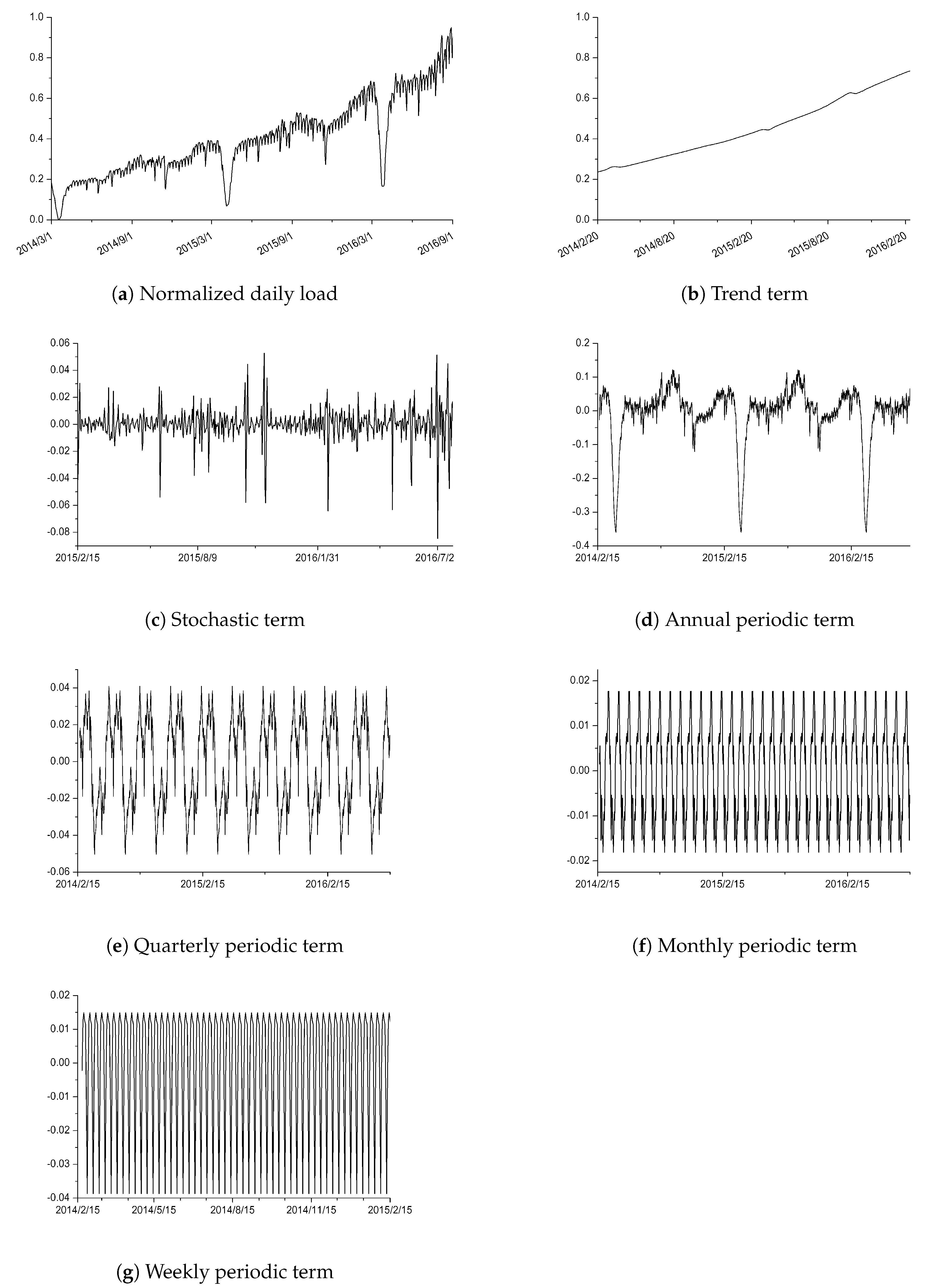
The electrical load pattern is heavily influenced by both internal factors (e.g., users’ consumption pattern) and external factors (e.g., weather, days of the week, and special events), which makes it uncontrollable. On the one hand, the electrical load patterns show randomness due to the influence of random factors (such as weather change, special events, etc.). On the other hand, it also behaves regularly due to the relative certainty of users’ power consumption pattern. In general, the electrical loads can be decomposed into trend term, periodic term, and stochastic term [5,27]. As shown in Figure 1, the normalized daily electrical load of Hangzhou city in eastern China from 1 January 2014 to 31 March 2017 (Figure 1a) is decomposed into trend term (Figure 1b), stochastic term (Figure 1c) and periodic term, which can be further decomposed into annual periodic term (Figure 1d), quarterly periodic term (Figure 1e), monthly periodic term (Figure 1f) and weekly periodic term (Figure 1g).

After statistical analysis of power load, we can observe that:

(i) Figure 1d–g clear shows that the electricity load has quasi-periodicity of various time spans, i.e., the load patterns show great similarity over years, seasons, months, and weeks.

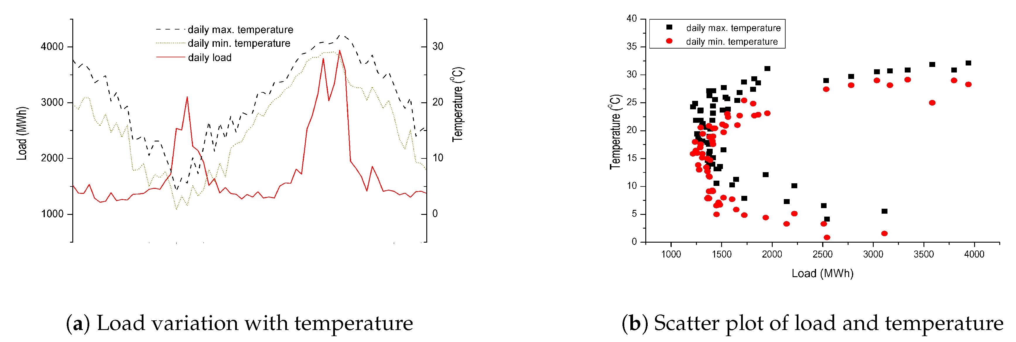
(ii) Electricity consumption is closely related with temperature. The daily electricity consumption in megawatt hour (MWh) and the temperature in degree Celsius (°C) are presented in Figure 2a, from which it is clear that the electricity consumption in summer and winter is much higher than that in spring and autumn. More specifically, the load variation with the daily maximum/minimum temperature is illustrated in Figure 2b in the form of scatter plot, from which we can see that load increases significantly in both higher (daily minimum temperature is higher than 27 °C) and low temperature zones (daily maximum temperature lower than 6 °C).

Further, we use Pearson correlation coefficient to analyze the correlation between temperature and electrical load, which is defined by

$$\rho =\frac{{\sum }_n\left(L{}_d\left(n\right)-\overline{L}{}_d\left)\left(T{}_a\left(n\right)-\overline{T}{}_a\right)\right.\right.}{\sqrt{{\sum }_n\left(L{}_d\left(n\right)-\overline{L}{}_d\left){}^2\left(T{}_a\left(n\right)-\overline{T}{}_a\left){}^2\right.\right.\right.\right.}},$$

(1)

where $L_d\left(n\right)$ is the daily load at the nth day, $\overline{L_d}$ is the mean of daily load sequence, and $T_a\left(n\right)$ and $\overline{T_a}$ are the average daily temperature and its mean, respectively.

Then, the student’s test (T-test) is utilized to test the null hypothesis of “population correlation coefficient is 0”. If T-test is significant, the null hypothesis is rejected and we say temperature and electrical load are linearly dependent; otherwise, they are considered to be linearly independent. Pearson correlation test results, listed in

Table 1. Pearson correlation test of load and temperature.

Variable	Significance	Correlation
Max. temperature-electrical load	0.033	Significant correlation at 0.05
Min. temperature-electrical load	0.005	Significant correlation at 0.01

, show that a high linear dependence exists between daily temperature and load. Therefore, temperature data will help to improve the prediction.

(iii) Data imbalance problem. It can also be observed from the scatter plot in Figure 2b that there are fewer samples in higher/lower temperature zones than those in mild temperature zones.

(iv) Randomness induced by special events. As can be seen in Figure 1a, the load reaches its lowest point in February every year, which is due to the great reduction of electricity consumption during the Spring Festival holiday. In addition, there was an unusual drop in August 2016 due to the strict power restrictions on enterprises during the G20 Summit. These special events have great impact on the load pattern, thus using the load with similar pattern as training samples can improve the accuracy of prediction.

According to the above features of electrical load, we can improve the prediction performance of STLF by: (a) fully exploiting the quasi-periodicity with various periods of electrical load; (b) accurately learning and representing the complicated load patterns; (c) overcoming the data imbalance problem of electrical load; and (d) exploring the effect on load by external factors such as temperature, day of week, and special events.

3. Deep Ensemble Learning Model Based on LSTM within Active Learning Framework

Taking these characteristics into consideration, an enhanced deep ensemble learning model is developed, which features: (a) A LSTM-based deep learning model is used to explore the complicated patterns hidden in electrical load. (b) The selector of the active learning framework actively selects several key samples with the most similar patterns to distill quasi-periodicity information, and eliminates the negative effect of data imbalance. (c) An ensemble model integrating LSTM and MLP greatly improves the model capacity of deep neural network with a little penalty on complexity.

3.1. Improved Active Learning Framework

Active learning [28,29] was proposed for model training with sufficient data but few labeled samples. Its main idea is to select the key samples from the unlabeled dataset that affect the learning performance mostly, and then label these key samples artificially. The theoretical basis of active learning is that the model usually depends on only a small number of key samples and most of the useful information is covered by these key samples. If these key samples are selected to train the model, all other samples can be ignored so that the model training is much more efficient. Usually, active learning system consists of a learner and a selector. The learner often employs a supervised learning algorithm to train the model from labeled data, and the selector selects key samples for the learner after labeling. The key of active learning is how to select the key samples. Comparing with the passive learning methods which train the model from all given samples, active learning method has more rapid convergence and overcomes the data imbalance problem.

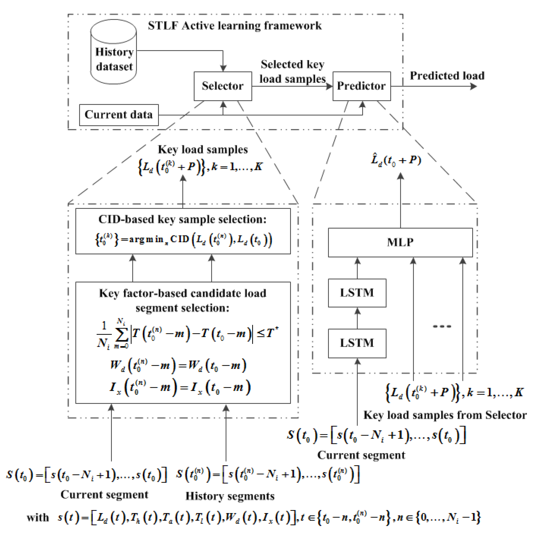
Inspired by actively selecting key samples to accelerate model training and mitigate data imbalance, an active learning framework is developed, and its structure is shown at the upper part of Figure 3. It is well known that an artificial neural network will produce similar output when similar input is given. For STLF, the similarity of load shape is chosen and then the key samples are those have similar curve shape to the one to be forecasted. These key samples are inputted to the predictor for training the STLF model together with current load segment and corresponding attributes including temperature, holidays or not.

3.2. The Selector Based on Load Shape Similarity

The selector actively selects several load segments most similar to the current load segment as the training samples, thus it is very important to employ a suitable similarity measurement. In this paper, the similarity of load pattern is based on the similarity of load curve, whose theoretical basis is as follows: (a) The trend of load will continue in short term, that is, it is of high possibility that the loads behave similarly in the near future if they are alike in the previous several days. (b) The load pattern is strongly affected by several external factors such as temperature, day of week, and special events. When these key external factors are the same, their effects on the load will be similar.

There are many metrics to measure the similarity of curve shape such as Euclidean distance, Fechet distance [30], and Hausdorff distance [31]. For good balance between performance and computation complexity, complexity-invariant distance (CID) is deployed, which is much easier to compute than Fechet distance and Hausdorff distance. CID is a modified Euclidean distance, which weights the Euclidean distance by the curve complexity factor (CCF) [32]. The CCF comes from a physical intuition: if a curve is stretched to a straight line, a more complicated curve would produce a longer straight line than a simple one. The CID of two daily load curves ${\mathit{L}}_d\left(t_0\right)$ and ${\mathit{L}}_d\left(t_1\right)$ is defined by

$$\mathrm{CID}({\mathit{L}}_d\left(t_0\right),{\mathit{L}}_d\left(t_1\right))=ED({\mathit{L}}_d\left(t_0\right),{\mathit{L}}_d\left(t_1\right))·CF({\mathit{L}}_d\left(t_0\right),{\mathit{L}}_d\left(t_1\right)),$$

(2)

where $ED({\mathit{L}}_d\left(t_0\right),{\mathit{L}}_d\left(t_1\right))=\sqrt{{\sum }_{n=1}^N{(L_d(t_0-n)-L_d(t_1-n))}^2}$ is the Euclidean distance between curves ${\mathit{L}}_d\left(t_0\right)$ and ${\mathit{L}}_d\left(t_1\right)$ of length N, and $CF({\mathit{L}}_d\left(t_0\right),{\mathit{L}}_d\left(t_1\right))$ is the CCF defined by

$$CF({\mathit{L}}_d\left(t_0\right),{\mathit{L}}_d\left(t_1\right))=\frac{max\{CE\left({\mathit{L}}_d\left(t_0\right)\right),CE\left({\mathit{L}}_d\left(t_1\right)\right)\}}{min\{CE\left({\mathit{L}}_d\left(t_0\right)\right),CE\left({\mathit{L}}_d\left(t_1\right)\right)\}},$$

(3)

where $CE\left({\mathit{L}}_d\left(t_0\right)\right)=\sqrt{{\sum }_{n=0}^{N-2}{(L_d(t_0-n)-L_d(t_0-n-1))}^2}$.

Similarity metrics of external factors are vital for the selection of key samples as well. Since the load pattern in higher/lower temperature zones differs greatly from that in mild temperature zones, the similarity metric differs according to the daily temperature. Specifically, if the difference of absolute mean daily temperature related to two load segments is less than a threshold $T_h$, these two load segments will be considered to be highly similar. In the case shown in Figure 2a, electrical load fluctuates sharply even the temperature changes mildly in sensitive temperature zone, while it is much insensitive to the temperature change in the mild temperature zone. Therefore, the value of threshold $T_h$ should be different for these two kinds of temperature zones. In the above example, the value of threshold is 0.5 and 5 for sensitive and insensitive temperature zones, respectively. It should be noted that both sensitive temperature zone and threshold are determined by the statistical analysis of load and corresponding temperature data.

3.3. Deep Ensemble Learning Predictor based on LSTM and MLP

The full utilization of load’s quasi-periodicity information can enhance LSTF. For a long period, it is not necessary to input all the time series, but only the most similar segments as training samples. There exists high correlation between these selected load segments and the current one so that they cannot be merged into a longer series as input to the LSTM. This is because the LSTM model trained by these very similar series will be very similar. At the same time, for LSTM models, the training complexity increases much faster than the input length. Therefore, it is more reasonable to adopt ensemble learning.

LSTM has been employed to learn the inner temporal variation pattern of the load, and K selected key daily load by selector are combined to fed the predictor so as to extract the information contained in the quasi-periodicity of any period. The structures of both Selector and Predictor are depicted in the lower part of Figure 3, where the input of LSTM, $\mathit{S}\left(t_0\right)=\left[\mathit{s}(t_0-N_i+1),\mathit{s}(t_0-N_i+2),\dots ,\mathit{s}\left(t_0\right)\right]$, is a segment for $N_i$ consecutive days. The $(N_i-n)$th element of $\mathit{S}\left(t_0\right),\mathit{s}(t_0-n)=\left[L_d(t_0-n),T_h(t_0-n),T_a(t_0-n),T_l(t_0-n),W_d(t_0-n),I_x(t_0-n)\right]$, is a six-tuple vector consisting of daily electrical load $L_d(t_0-n)$, daily maximum temperature $T_h(t_0-n)$, daily mean temperature $T_a(t_0-n)$, daily minimum temperature $T_l(t_0-n)$, day of the week $W_d(t_0-n)$, and date type $I_x(t_0-n)$. Among them, $I_x(t_0-n)$ corresponds to weekday, weekend, long holiday (such as National Day and Spring Festival in China, or Easter, Christmas, etc.) and major event (such as the Olympics, OPEC, G20 and other events that greatly affect the load patterns).

The Selector chooses K samples, $\mathit{S}(t_0^{\left(k\right)}),k=1,2,\dots ,K$, and outputs the daily load elements at day $t_0^{\left(k\right)}+P$, $L_d(t_0^{\left(k\right)}+P),k=1,\dots ,K$. MLP combines outputs from both LSTM and Selector to estimate $L_d(t_0+P)$, the daily load at day $t_0^{\left(k\right)}+P$. The training process is listed below:

Step 1: Data preprocessing.

• Normalizing the electrical load.

  $${\overline{L}}_d\left(t\right)=\frac{L_d\left(t\right)-{min}_j\left\{L_d\left(j\right)\right\}}{{max}_j\left\{L_d\left(j\right)\right\}-{min}_j\left\{L_d\left(j\right)\right\}}.$$

  (4)
• One-hot encoding day of the week and date types;
• Splitting data into training set and test set;

Step 2: Initiating model parameters

• Initial parameters of LSTM network: number of LSTM network layer L, number of input nodes $N_i$, number of hidden nodes $N_h$, number of output nodes $N_o$;
• Number of the most similar historical load segments: K;
• MLP parameters: Number of full connection layers Q, number of hidden layer nodes, activation function, cost function;

Step 3: Model training and parameter adjustment

• Key sample selection by Selector;
• Back-propagation through time (BPTT) is used to train the LSTM network;
• Error Back Propagation (BP) is deployed to train the MLP network;
• According to the training error curve and test error curve, the network is iteratively trained until the performance converges.

The procedure of key sample selection by Selector is listed below.

• Input: $\mathit{S}\left(t_0\right)=\left[\mathit{s}(t_0-N_i+1),\mathit{s}(t_0-N_i+2),\dots ,\mathit{s}\left(t_0\right)\right]$, current segment whose element is $\mathit{s}(t_0-n)=\left[L_d(t_0-n),T_h(t_0-n),T_a(t_0-n),T_l(t_0-n),W_d(t_0-n),I_x(t_0-n)\right]$;
• Output: $L_d(t_0^{\left(k\right)}+P),k=1,\dots ,K$, the daily load at days of $t_0^{\left(k\right)}+P$ of the selected K samples.

Step 1: Selection of candidate samples from dataset to meet the following three conditions

• Condition 1: $\frac{1}{N_i}{\sum }_{m=0}^{N_i}|T(t_0^{\left(n\right)}-m)-T(t_0-m)|\le T^{*}$, where $T\in \{T_h,T_a,T_l\},T^{*}=5$ for $T=T_a$ and $T^{*}=0.5$ for $T\in \{T_h,T_l\}$;
• Condition 2: $W_d(t_0^{\left(n\right)}-m)=W_d(t_0-m),m=0,1,\dots ,N_i-1$;
• Condition 3: $I_x(t_0^{\left(n\right)}-m)=I_x(t_0-m),m=0,1,\dots ,N_i-1$.

Step 2: Calculation of CID distance of the candidate segment to the input segment according to Equation (2) by $d\left(n\right)=CID(L_d(t_0^{\left(n\right))},L_d\left(t_0\right))$.

Step 3. Choose of Key samples

• Selecting K candidate segments with the minimum CID distances as the key samples denoting by $\{\mathit{S}(t_0^{\left(k\right)})\},k=1,2,\dots ,K$;
• Outputting the daily load $\{L_d(t_0^{\left(k\right)}+P)\},k=1,2,\dots ,K$.

4. Experiment and Result Discussion

4.1. Experiment Settings

The proposed model was evaluated on an open dataset, which contains the daily load (https://www.torontohydro.com) and weather records (http://climate.weather.gc.ca) of Toronto, Canada from June 2002 to July 2016. Cross-validation was adopted for performance evaluation, i.e., the dataset was partitioned into two isolated subsets: training dataset and test dataset. The test data were not used in training model for fair performance comparison. The partition ratio of training data and test data was 7:3.

Several classic STLF algorithms were also simulated for reference, including MLP, ARIMA, SVR, LSTM. Tensorflow-gpu and scikit-learn were used in Python simulation environment.

4.2. Hyper-parameters Optimization

The optimization of hyper-parameters of STLF models is to optimize the STLF performance in the form of mean absolute percent error (MAPE), which is defined by

$$MAPE=\frac{1}{N}\sum _{n=1}^N\left|\frac{{\widehat{L}}_d\left(n\right)-L_d\left(n\right)}{L_d\left(n\right)}\right|\times 100\%,$$

(5)

where ${\widehat{L}}_d\left(n\right)$ is the forecasted value of the electrical load $L_d\left(n\right)$ at the nth day.

Since the training complexity and the required training samples increase sharply when the layers of LSTM network increase, good balance between MAPE and complexity is concerned for the selection of layers of LSTM network. In other words, when the MAPE performance increases slightly at the cost of sharp increase of complexity, then fewer layers are employed.

The procedure of hyper-parameters and thresholds optimization consists of two phases.

Phase 1: Optimizing standard LSTM model.

The initial settings of STLF models are based on the statistical analysis of dataset, and the optimization procedure of hyper-parameters are based on the cross-validation method.

Through statistical analysis of daily load, typical period of seven is observed. Then, the initial number of input nodes is set to be seven while the number of layers iterates from one. After several rounds of performance evaluation for hyper-parameters adjustment, the settings of the standard LSTM model are determined as $L=2$, $N_i=15$ for seven days forecasting and $N_i=8$ for other days forecasting, and $N_h=8$.

Phase 2: Optimizing the proposed model. The LSTM network in the proposed model has the same setting as standard LSTM, and the optimization of MLP network settings follows four steps.

The first step is to choose thresholds $T^{*}$ for different temperature zones. According to the scatter plot of daily load and temperatures, the high, low and mild temperature zones are defined. Since the mild temperature zone holds large temperature variation, its average temperature variation is calculated with result of 4.26 °C within a week and 5.91 °C within two weeks. Then, $T^{*}=5$ is chosen as the initial threshold for mild temperature zone. After computing the ratios between daily variation and temperature variation in three temperature zones, it is found that the ratio in sensitive temperature zones is about ten times of that in mild temperature zone, from which $T^{*}=0.5$ is chosen as the initial value for sensitive temperature zones.

The second step is to initiate the number of key samples. After counting the number of daily segments with high similarity defined by thresholds $T^{*}$ for different temperature zones, the minimum number of highly similar daily load segments within high temperature zones is 6, and $K=6$ is chosen to be the initial value.

The third step is to initiate the layers and activation function of MLP. The number of layers begins from $Q=1$, and the activation function is chosen from sigmoid function and linear function.

The final step is to optimize hyper-parameters iteratively via cross-validation by changing the parameter settings such as K, Q, and activation function. The final model settings are listed in

Table 2. Model parameter settings.

Days of prediction	$P=1,3,5,7$
Layers of LSTM	$L=2$
Input nodes of LSTM	$N_i=8$ when $P=1,3,5$ $N_i=15$ when $P=7$
Hidden nodes of LSTM	$N_h=8$
Output nodes of LSTM	$N_o=N_i$
No. of selected load segments	$K=4$
Full connection layers of MLP	$Q=1$
Activation function of MLP	linear activation function

.

4.3. Results and Analysis

MAPE was used to evaluate the forecasting performance of STLF.

Table 3. MAPE performance comparison.

Algorithm	$\mathit{P}=1$	$\mathit{P}=3$	$\mathit{P}=5$	$\mathit{P}=7$
MLP	5.5%	18.1%	27.91%	35.10%
ARIMA	14.10%	16.90%	18.21%	19.50%
SVR	4.3%	6.90%	7.3%	7.1%
LSTM	4.10%	6.25%	6.88%	7.15%
Proposed model	2.98%	4.87%	4.91%	5.10%

lists the simulation results, from which we can observe:

• The proposed model outperforms all reference STLF models in all simulated scenarios, which verifies the effectiveness of the proposed model.
• LSTM holds better performance than the other reference models. However, as the prediction time span increases, LSTM degrades significantly. This indicates that the length of input load segment is not enough to accurately predict the power load after seven days, such that longer input segment is needed, which further verifies the advantage of the proposed model.
• MLP model shows a similar trend as LSTM, that is, as the prediction time span increases, the predicted performance degrades rapidly. Its performance is limited by both insufficient input load segment and the limited learning capability.
• Although ARIMA model is enhanced for non-stationary series by difference operation, its learning capability is insufficient for electrical load featuring typical non-stationarity such that it is difficult to accurately model complicated and diverse patterns.
• SVR shows good learning ability whose MAPE performance decreases slowly with the increase of prediction time. The main reason is that it learns from all data, but only selects key samples (support vectors), thus has the ability of active sample selection similar to active learning.

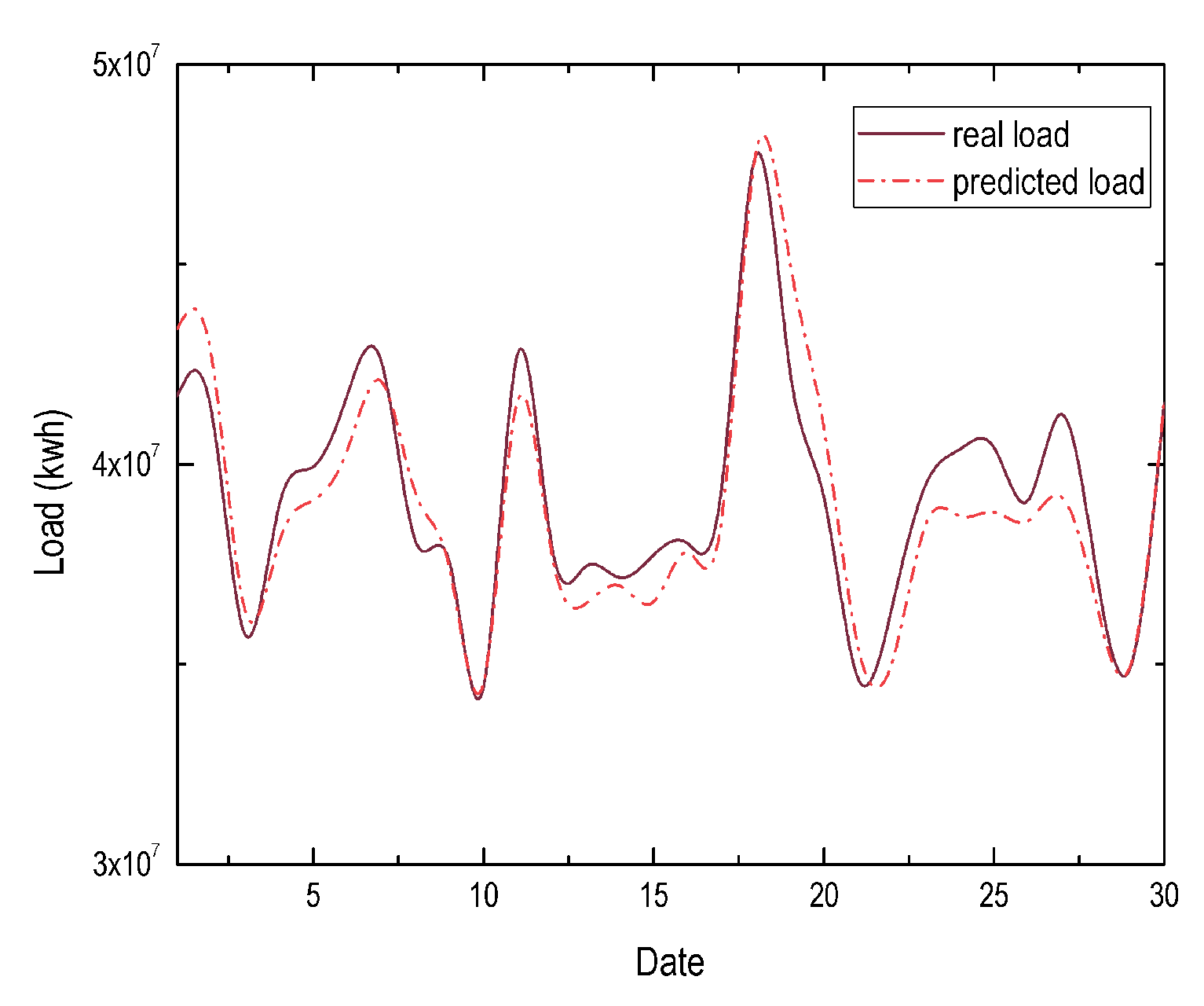
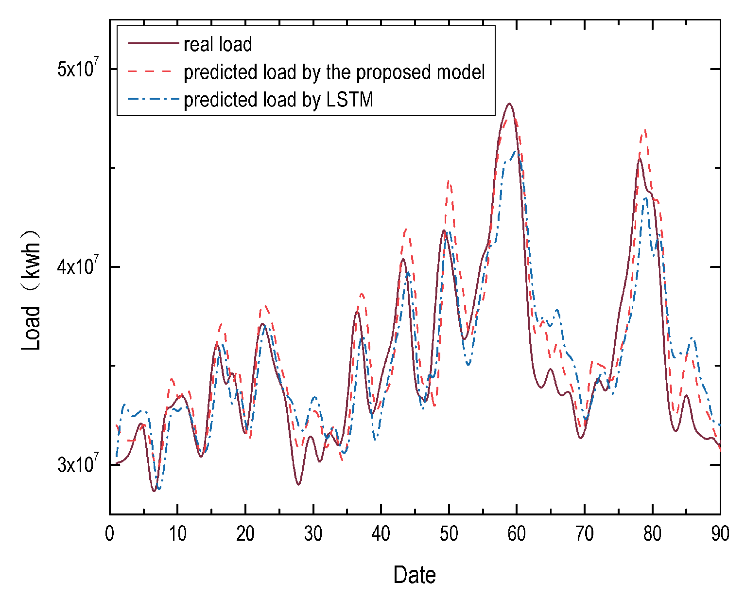
Since the load fluctuates sharply in sensitive temperature zones, it is necessary to evaluate the performance in different seasons. Figure 4 and Figure 5 present the STLF results in spring and summer, and the results show that the proposed model achieves MAPE of $1.86\%$ in spring and $4.9\%$ in summer, which are much lower than all reference models. Specifically, the MAPE results of ARIMA, MLP, SVR and LSTM are $9.29\%,2.77\%,2.53\%$, and $2.48\%$ in spring, and $21.8\%,7.98\%,6.5\%$, and $6.3\%$ in summer, respectively. These results also verify the load patterns in sensitive temperature zones are more complicated, and the proposed model can learn complicated patterns much better.

5. Conclusions

STLF is of great significance to the smart grid, which is the basis of intelligent dispatching, demand-side response and stable operation of the power grid. Due to complicated load patterns such as quasi-periodicity with large time span and randomness induced by many external factors, classic regression models and shallow neural networks have difficulty accurately modeling the complicated electrical load pattern. LSTM-based deep learning model, presenting state-of-the-art performance, cannot avoid the vanishing gradient problem and has a limit on the length of input sequence, which results in the inability to exploit quasi-periodic information of large time span. Furthermore, the data imbalance problem of load patterns degrades LSTM. Therefore, a deep ensemble learning model combined LSTM and MLP within the active learning framework is developed in this paper. By selecting several historical load segments most similar to the current one to be predicted, the quasi-periodic information of any time span can be fully utilized, and the imbalance problem among load patterns is eliminated at the same time. The deep ensemble learning-based predictor combines LSTM and MLP to achieve better prediction performance by ensemble learning with little increase of training complexity. Experiments have been done over an open dataset, and the results show the proposed model outperforms the existing classic STLF models.