Harmonic Detection for Power Grids Using Adaptive Variational Mode Decomposition

Abstract

The harmonic pollution problem in power grids has become increasingly prominent with the large-scale application of power electronic equipment, nonlinear loads, and renewable energy. This study proposes a method based on adaptive variational mode decomposition (AVMD) and Hilbert transform (HT) that is applicable to harmonic detection in power system. The AVMD method constructs and solves the constrained variational model. Then, a single-frequency harmonic component with stable features can be obtained. The proposed method can effectively avoid the recursive process in empirical mode decomposition (EMD). In this study, the variational mode decomposition algorithm is used to obtain the periodic harmonic components concurrently. Subsequently, the characteristic parameters of each harmonic component are extracted via HT. Simulation analysis and measured data verify the validity and feasibility of the proposed algorithm. Compared with the detection results obtained using the EMD algorithm, the proposed method is proven to exhibit stronger applicability to harmonic detection in power system.

1. Introduction

In recent years, more and more power electronic equipment is put into operation. While improving the flexibility and reliability of power grid operation, these power electronic devices also generate a large amount of harmonic pollution, which affects the power quality of the power grid [1,2,3,4]. Power system harmonic detection is an important prerequisite to harmonic source localization and harmonic control. Therefore, accurate harmonic detection is highly significant in ensuring the stable and high-quality operation of a power grid [5,6].

Fast Fourier transform (FFT) [7] is the earliest classical method applied to harmonic detection. However, this method is generally suitable only for analyzing stationary signals. For the analysis of non-stationary oscillation in power systems, spectral leakage and the fence effect [8,9] will occur, which limited the application of FFT algorithm in power system harmonic detection. Based on the FFT algorithm, the short-time Fourier transform (STFT) [10,11,12] extracts harmonic parameters by reducing the width of the frequency window. However, the STFT algorithm has a low frequency resolution. In [13,14], the windowed Fourier transform (WFT) algorithm was used to improve the detection precision of the FFT method by selecting an appropriate window function; however, this algorithm complicates the calculation process and may introduce false components. Through the effort of experts and scholars, the nonlinear analysis method has achieved productive results and has been successfully applied to power system harmonic detection. The wavelet transform method exhibits good time-frequency characteristics and is suitable for the time-frequency analysis of harmonic signals [15,16]. However, the accuracy of harmonic detection is affected due to the poor resolution of the high-frequency band. Meanwhile, the frequency is aliased, which also reduces the accuracy of detection results [17]. The Hilbert-Huang transform (HHT) algorithm is particularly effective in dealing with nonlinear and non-stationary signals and does not require selecting the basis function before calculation. The algorithm firstly uses empirical mode decomposition (EMD) algorithm to obtain the intrinsic mode function (IMF) components, and then the Hilbert transform is used to extract harmonic parameters. In practical applications, however, detection accuracy is considerably affected by noise, which causes serious mode-mixing problems [18,19,20]. The local mean decomposition (LMD) algorithm [21,22] uses division to replace the subtraction in the process of acquiring the IMF components in EMD algorithm. Although the computational efficiency has improved, the mode-mixing problem has not fundamentally been solved.

To address the mode-mixing problem in harmonic detection using EMD algorithm, this paper proposes a new method based on the adaptive variational mode decomposition (AVMD) algorithm. The variational mode decomposition (VMD) algorithm is an effective harmonic signal extraction method that is primarily used in the fault detection of mechanical components, such as bearings and gears [23,24,25]. The VMD algorithm, which differs completely from the recursive decomposition of the EMD algorithm, constructs the constrained variational model and searches for the optimal solution to detect harmonic signals, and the harmonic components are detected concurrently. The algorithm exhibits good robustness to noise and avoids the mode-mixing problems in the EMD algorithm to a certain extent. However, the number of decomposition (K) must be set in advance in the AVMD algorithm. The rationality of the set decomposition number has a significant impact on the harmonic detection results, which limits the adaptability of the VMD algorithm. In [26], the particle swarm optimization (PSO) algorithm was used to determine the value of decomposition, but PSO consumes too much time, and the result depends on the selected optimization algorithm. In [27], the optimal value of K was selected using the double threshold method; however, the calculation result depends on the threshold and is subjective.

FFT algorithm is a classical algorithm for harmonic detection. According to the number of peaks in FFT spectrum, the harmonic components in the signal can be determined. However, only the harmonic frequencies can be obtained, and the exact amplitudes and phases of harmonics cannot be obtained from the FFT spectrum. Based on the FFT spectrum, from which the decomposition number can be determined, a harmonic detection method based on AVMD and Hilbert transform is proposed. The AVMD algorithm is firstly used to decompose the multi–harmonic coupled signal to obtain harmonic components in time domain, and then use the Hilbert transform to detect the harmonic amplitudes, frequencies and phases of each component. The proposed method improves adaptability to noise. In addition, compared with the frequency-domain approaches, such as FFT, the time-domain decomposition method proposed in this paper can obtain harmonic frequencies, while the accurate harmonic amplitudes and phases can be obtained as well.

The remainder of this paper is organized as follows. Section 2 introduces the basic theory and decomposition process of the AVMD algorithm based on the FFT spectrum. Section 3 presents harmonic component detection based on HT. Section 4 provides the simulation results of the test signals and the measured data. Finally, Section 5 concludes the study.

2. Proposed AVMD Algorithm for Harmonic Detection

The nonlinear signal analysis represented by the EMD algorithm is essential for obtaining intrinsic components via recursive decomposition, which causes the accumulation of errors during the decomposition process and the poor accuracy of the decomposition results [28,29]. In contrast with the EMD method, the VMD algorithm is a completely non-recursive analysis method. The non-recursive method converts the signal decomposition process into the construction and solution of the constrained variational model and realizes the flexible decomposition of a signal in the frequency domain. The proposed method is also highly robust to noise and effectively avoids the mode-mixing and false mode problems in EMD. Thus, the proposed method can effectively detect harmonic components in the signal.

2.1. VMD AlgorithmTheory

The VMD algorithm transforms the signal decomposition process into the establishment and solution of the constraint variational model, thereby adaptively decomposing the multi-harmonic coupled signal into a multiple of bland-limited intrinsic mode functions (BLIMFs); each intrinsic component has a tightly distributed characteristic around its respective central frequency [23].

The constrained variational model contains equality and inequality constraints. In the equality constraint, the sum of the BLIMFs components is equal to the decomposed signals. In the inequality constraint, the sum of the estimated bandwidths for each BLIMFs component is the smallest. The constrained variational model that corresponds to the decomposition process of the response signal (f) is given as

$$\{\begin{array}{l}\underset{\left\{u_k\right\},\left\{{\omega }_k\right\}}{\min }\left\{{\displaystyle \sum _{k=1}^K\parallel {\partial }_t[(\delta (t)+\frac{j}{\pi t})\ast u_k(t)]e^{-j{\omega }_{k}t}{\parallel }_2^2}\right\}\\ s.t.{\displaystyle \sum _{k=1}^K{u}_k}=f\end{array}$$

(1)

where δ(t) is a unit pulse function; * represents convolution; {u_k} = {u₁,…,u_K} are the decomposed modal components for each BLIMFs; {ω_k} = {ω₁,…,ω_K} are the central frequencies for each BLIMFs.

To obtain the optimal solution for Formula (1), a quadratic penalty term α and Lagrange multiplier λ are used to render the problem in Equation (1) unconstrained, then the constructed augmented Lagrange function can be described as

$$L(\{{\mathit{u}}_k\},\{{\mathbf{\omega }}_k\},\lambda )=\alpha {\displaystyle \sum _{k=1}^K\parallel {\partial }_t[(\delta (t)+\frac{j}{\pi t})\ast u_k(t)]\ast e^{-j{\omega }_{k}t}{\parallel }_2^2}+\parallel f(t)-{\displaystyle \sum _{k=1}^K{u}_k(t){\parallel }_2^2}+\langle \lambda (t),f(t)-{\displaystyle \sum _{k=1}^K{u}_k(t)}\rangle$$

(2)

where α is the penalty factor, and λ is the Lagrange multiplier.

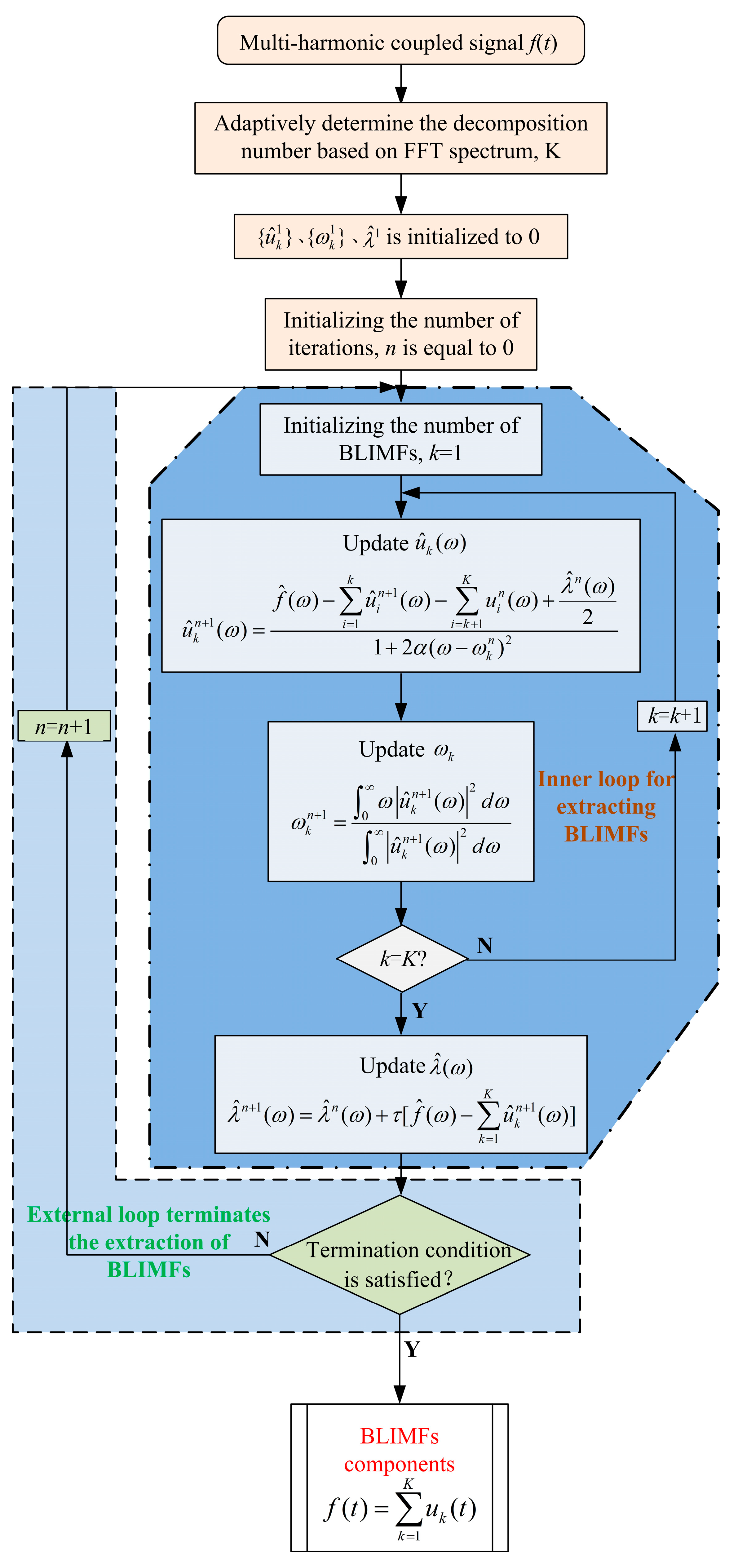
The optimal solution for the constrained variational model is obtained using the alternating direction multiplier algorithm (ADMM) [30,31]; that is, the intrinsic modal component of each finite bandwidth is extracted. The extraction process consists of two loops. The inner loop is for BLIMFs component extraction and harmonic parameter detection. The outer loop ensures identification accuracy for each BLIMFs component.

2.2. Inner Loop

For the inner loop, the intrinsic modal component (u_k) of the finite bandwidth, the modal center frequency (ω_k), and the Lagrange multiplier (λ) are sequentially updated in accordance with Equations (3), (4), and (5), respectively. The BLIMFs can be obtained through the following implementation process.

Step 1: $\{{\widehat{u}}_k^1\}$,$\left\{{\omega }_k^1\right\}$, and ${\widehat{\lambda }}^1$ are initialized; and the initial value of the iteration’s number (n) is set to 0. The decomposition mode number (K) is determined using the FFT algorithm.

Step 2: The first process of the inner loop is performed, and the modal component (u_k) and the center frequency (ω_k) are updated step by step in accordance with Formulas (3) and (4) as

$${\widehat{u}}_k^{n+1}(\omega )=\frac{\widehat{f}(\omega )-{\displaystyle \sum _{i=1}^k{\widehat{u}}_i^{n+1}(\omega )-{\displaystyle \sum _{i=k+1}^K{u}_i^n(\omega )+\frac{{\widehat{\lambda }}^n(\omega )}{2}}}}{1+2\alpha {(\omega -{\omega }_k^n)}^2}$$

(3)

$${\omega }_k^{n+1}=\frac{{\displaystyle {\int }_0^{\infty }\omega {\left|{\widehat{u}}_k^{n+1}(\omega )\right|}^{2}d\omega }}{{\displaystyle {\int }_0^{\infty }{\left|{\widehat{u}}_k^{n+1}(\omega )\right|}^{2}d\omega }}$$

(4)

Step 3: Step 2 is repeated until the decomposition number is equal to K. The first process of the inner loop ends, and the second process is performed to update the Lagrange multiplier (λ) in accordance with Equation (5) as

$${\widehat{\lambda }}^{n+1}(\omega )={\widehat{\lambda }}^n(\omega )+\tau [\widehat{f}(\omega )-{\displaystyle \sum _{k=1}^K{\widehat{u}}_k^{n+1}(\omega )}]$$

(5)

where ${\widehat{u}}_k^{n+1}(\omega )$ represents the Wiener filtering of the signal, ^ represents the Fourier transform, and τ is the fidelity coefficient.

2.3. OuterLoop

To ensure identification accuracy for each BLIMFs component, the outer loop process sets a termination condition for ending the harmonic detection process. The termination condition is described as

$${\displaystyle \sum _{k=1}^K\frac{\parallel {\widehat{u}}_k^{n+1}(\omega )-{\widehat{u}}_k^n(\omega ){\parallel }_2^2}{\parallel {\widehat{u}}_k^n(\omega ){\parallel }_2^2}<\epsilon }$$

(6)

If the extracted BLIMFs components satisfy the Formula (6), then the iteration is terminated, that is, the entire modal decomposition is completed. Otherwise, the results of the inner loop calculation are used as the initial values of the iteration, the iteration returns to the inner loop, and Steps 1 to 3 are repeated. The decomposition results will be obtained only after the termination condition of Formula (6) is satisfied.

The detailed harmonic decomposition process is shown in Figure 1.

3. Harmonic Detection Based on the AVMD Algorithm in Power System

When the VMD algorithm is used to decompose a signal, the decomposition number (K) exerts greater impact on the decomposition effect when it is properly set. If the value of K is greater than the actual number of BLIMFs components, then a false harmonic component is generated in the result. Meanwhile, a small K will lead to insufficient decomposition; that is, the dominant harmonic components contained in the signal are not completely decomposed. Therefore, to obtain accurate harmonic components, an appropriate value of K is a key parameter in decomposition using the VMD method [23].

The BLIMFs components decomposed by the VMD algorithm exhibit a tight distribution around the center frequency [23]. By analyzing the characteristics of the signal to be decomposed in the frequency domain and combining the properties of the FFT algorithm, the value of the decomposition number (K) used in the VMD algorithm is adaptively determined on the basis of the number of peaks in the FFT spectrogram.

For the time-domain signal, there are always no evident features from external characteristics. However, the features are significant when the time-domain signal is transformed to the signal in frequency domain. Therefore, converting time-domain signals to frequency-domain signals for analysis is a common analytical method for power system. FFT algorithm is a widely used transformation tool (Fourier transform theory is relatively mature) and is also a relatively common tool for converting time-domain signals to frequency-domain analysis.

The quantitative analysis of the amplitude of the harmonic components with frequency ω is realized through FFT algorithm, and the harmonic components in the response signal are obtained.

The active power of an actual power grid and its FFT spectrogram are shown in Figure 2. The number of harmonics in the signal is determined by analyzing the number of peaks in the FFT spectrogram. Consequently, the decomposition number (K) can be determined using the AVMD algorithm in accordance with the number of peaks in the FFT spectrogram.

The multi-harmonic coupled signal in a power system is a superimposed signal with fixed amplitude, frequency, and phase. When the coupled signal is decomposed using the AVMD algorithm, several relatively stable single-frequency harmonic components will be obtained, thereby providing good components for HT analysis and ensuring accurate results for harmonic detection [32,33].

After decomposition is executed by AVMD, the harmonic parameters of each BLIMFs component are obtained via HT. HT is conducted for any BLIMFs component I(t), and the following formula is obtained [32]

$$I^{\ast }(t)=\frac{1}{\pi }P{\displaystyle {\int }_{-\infty }^{+\infty }\frac{I(\tau )}{t-\tau }d\tau }$$

(7)

where P is the Cauchy principal value integral.

Thus, the analytic signal of I(t) is expressed as

$$g(t)=I(t)+j{I}^{*}(t)=A(t)e^{j\delta (t)}$$

(8)

where A(t) and δ(t) are the instantaneous amplitude and phase, respectively, which can be written as

$$\{\begin{array}{l}A(t)=\sqrt{I^2(t)+I^{*2}(t)}\\ \delta (t)=\arctan \frac{I^{*}(t)}{I(t)}\end{array}$$

(9)

The harmonic signal in a power grid is generally a periodic signal with fixed amplitude and frequency. On the basis of the feature, the harmonic signal can be expressed as

$$f(t)=A\cos (2\pi ft+{\theta }_0)$$

(10)

where A, f, and θ₀ are the amplitude, frequency, and phase of the harmonic signal, respectively.

For the Formulas (8) and (10), the following can be obtained in accordance with the principle that the corresponding coefficients are equal

$$\{\begin{array}{l}A(t)=A\\ \delta (t)=2\pi ft+{\theta }_0\end{array}$$

(11)

Considering environmental factors and measurement noise, δ(t) and t cannot guarantee a strict linear relationship, and the least squares fitting method [34] is used for Formula (11). Therefore, harmonic characteristic parameters, including instantaneous frequency, amplitude, and phase can be detected.

Furthermore, the harmonic parameters can be extracted through the following process.

Step 1: The value of harmonic decomposition in the AVMD algorithm is adaptively determined using the FFT spectrum; that is, the number of the peaks in spectrum is the harmonic components contained in the signal.

Step 2: After decomposition number (K) is determined, the multi-harmonic coupled signal is decomposed using the AVMD algorithm proposed in this study.

Step 3: The parameters of the decomposed harmonic components are extracted using the HT algorithm.

4. Results and Analysis

To demonstrate the efficiency and adaptability of the proposed method, this study selects the test signal and the measured harmonic signal of an actual power grid and uses MATLAB software for calculation and analysis.

To quantitatively evaluate the detection effect of the proposed method, the signal-to-noise ratio (SNR) index is typically used to characterize the accuracy of the detection result and is derived as

$$SNR=20\log \frac{\parallel y(k)\parallel }{\parallel y(k)-\widehat{y}(k)\parallel }$$

(12)

where $y(k)$ is the original signal, and $\widehat{y}(k)$ is the reconstructed signal.

4.1. Test Signal Analysis

The voltage and current signals in the power system are typically half-wave and symmetric. In general, they contain only 50 Hz power frequency and odd harmonic components. The higher the harmonic order, the smaller the harmonic amplitude. Therefore, harmonics with frequencies of 150 Hz and 250 Hz are superimposed on the fundamental signal of the 50 Hz power frequency, and noise of 30 dB is superimposed to consider the influence of measurement noise in the system. The test signal is described as

$$x(t)=\sin (2\pi \ast 50t)+0.2\sin (2\pi \ast 150t+\pi /6)+0.15\sin (2\pi \ast 250t+\pi /4)+\eta (t)$$

(13)

where $\eta (t)$ represents the noise component.

The sampling frequency is 10,000 Hz and the sampling point is 1000; thus, the simulation duration is 0.1 s. The time-domain response of the test signal is presented in Figure 3a. The harmonic characteristic of the test signal is significant. Then, the harmonic characteristic parameters are extracted using the proposed detection method.

Firstly, the number of decomposition (K) in the AVMD algorithm is determined according to the FFT spectrum analysis in Section 3. The corresponding FFT spectrum of the test signal is shown in Figure 3b. From the spectrum, we can infer that three peaks are obtained in the FFT spectrum analysis, namely, fundamental frequency, third harmonic, and fifth harmonic, on the basis of which we can determine 3 as the number of modal decomposition (K) in the AVMD algorithm, which is the same number of harmonics as the original signal. Meanwhile, the frequency components obtained by the decomposition are consistent with the frequency of the test signal, and the amplitudes of the third and fifth harmonics are considerably smaller than the fundamental signal, thereby indicating that using the FFT spectrum to determine the decomposition number in the AVMD algorithm is effective.

After the decomposition number is determined, signal x(t) is decomposed using the AVMD algorithm, and the result is shown in Figure 4a. The original test signal x(t) is decomposed into three harmonic components, namely, V-BLIMFs1, V-BLIMFs2, and V-BLIMFs3, which are fixed-frequency and equal-amplitude periodic components. The FFT algorithm is used to perform spectrum analysis on each component decomposed by the AVMD algorithm, and the results are shown in Figure 4b. The three BLIMFs components derived from AVMD decomposition have a fixed and stationary frequency, and the instantaneous amplitudes are close to the theoretical values.

To further illustrate the advantages of the proposed method in harmonic detection, the EMD decomposition results are used for comparative analysis. The results are provided in Figure 5a. As shown in the figure, four IMF components and one trend component are obtained. The number of IMF components is equal to the harmonic component of the test signal, but E-IMF1 does not completely contain the noise component of the test signal. Several noise components are also included in E-IMF2 and E-IMF3, thereby causing local distortion in the waveforms. To analyze the frequency-domain characteristics of the periodic components decomposed by EMD, the results are shown in Figure 5b. A significant mode-mixing phenomenon occurs; that is, the amplitude–frequency characteristic of the fundamental component contains the third harmonic component of 150 Hz, which reduces the accuracy of harmonic detection in the power system.

The HT-based harmonic detection method proposed in Section 3 is used to calculate the harmonic parameters of the components decomposed by AVMD and EMD, respectively, as given in

Table 1. Harmonic detection results of the test signal with SNR = 30 dB.

Algorithm	Harmonic	Frequency (Hz)	Amplitude	Phase (°)	Calculation Time (s)
Theoretical values	Fundamental	50	1.0000	0	-
	Third	150	0.2000	30.0000
	Fifth	250	0.1500	45.0000
AVMD + HT	Fundamental	49.99	0.9972	0.2416	4.144
	Third	149.93	0.1987	29.1432
	Fifth	250.01	0.1495	46.4916
EMD + HT	Fundamental	49.12	0.9726	0.3021	0.854
	Third	148.24	0.1432	28.7495
	Fifth	250.79	0.1846	48.5782
FFT	Fundamental	49.80	0.498	-	0.506
	Third	149.25	0.1024	-
	Fifth	250.31	0.0853	-

. Meanwhile, the detection results using FFT algorithm are also shown in Table 1. On the HP Z820 workstation (CPU: 2 * Intel Xeon E5-2600v3, 2.6 GHz; memory: 32 GB), the calculation time for extracting harmonic parameters using the above three algorithms is listed in Table 1. The calculated errors for the detection results obtained using the three methods are presented in

Table 2. Harmonic parameter errors using the two methods with SNR = 30 dB.

Parameter	Harmonic	AVMD + HT	EMD + HT	FFT
Frequency (Hz)	Fundamental	0.01	0.88	0.20
	Third	0.07	1.76	0.75
	Fifth	0.01	0.79	0.31
Amplitude	Fundamental	0.0028	0.0274	0.5020
	Third	0.0013	0.0568	0.0976
	Fifth	0.0005	0.0346	0.0647
Phase (°)	Fundamental	0.2416	0.3021	-
	Third	0.8586	1.2505	-
	Fifth	1.4916	3.5782	-

.

As shown in Table 1 and Table 2, we can know that the EMD algorithm is vulnerable to noise during the decomposition process, thereby resulting in a mode-mixing problem in the decomposition results. Hence, a difference exists between the extracted harmonic parameters and the theoretical parameters, and the accuracy of the identification results is considerably lower than those of the proposed harmonic detection method based on AVMD and HT. FFT algorithm can extract accurate harmonic frequencies, but the amplitude of the harmonics is inaccurate, and the phase of each harmonic component which is very useful for harmonic detection cannot be obtained. From the CPU calculation time results, we can know that FFT algorithm has the least calculation time, and the proposed AVMD takes the most time. Even so, the proposed method has the best detection accuracy among the three detection algorithms.

To further analyze the robustness to noise of the proposed method, the SNR is changed to 20 dB and 30 dB, and the harmonic parameters are extracted using the AVMD and EMD method. The results are provided in

Table 3. Harmonic detection results of the test signal with different SNRs.

SNR/dB	Harmonic	AVMD + HT			EMD + HT
		Frequency (Hz)	Amplitude	Phase (°)	Frequency (Hz)	Amplitude	Phase (°)
20	Fundamental	49.75	0.992	0.241	48.69	0.953	0.472
	Third	148.95	0.190	29.014	147.39	0.136	26.87
	Fifth	250.96	0.145	47.623	251.84	0.195	50.03
10	Fundamental	49.37	0.987	0.2380	47.39	0.905	0.642
	Third	148.32	0.188	28.982	145.87	0.114	25.06
	Fifth	249.06	0.138	47.058	253.06	0.220	53.41

. Compared with the EMD algorithm, the harmonic detection method proposed in this study exhibits better robustness to noise. Harmonic parameters can be accurately extracted even in an environment with a SNR of 10 dB.

The characteristic parameters in Table 1 extracted from the AVMD and EMD harmonic detection algorithms are used in signal reconstruction, and the reconstructed results are presented in Figure 6. The calculation results of the fitting accuracy based on the SNR are shown in

Table 4. Calculation results for SNR of the test signal.

Algorithm	SNR (dB)
AVMD + HT	35.9781
EMD + HT	7.9432

. A conclusion can be easily drawn that the test signal reconstructed by the proposed method exhibits good fit to the original signal, and the SNR calculation result is higher, thereby indicating that the reconstructed signal fits well with the original test signal.

4.2. Analysis of the Measured Data

To further verify the adaptability of the proposed algorithm in harmonic detection, the measured data of a 138 kV substation in Brazil is selected for calculation and analysis. The measured current signal containing harmonics is shown in Figure 7a.

Similar to the test signal analysis process, firstly, use the FFT spectrogram to determine the decomposition modal number (K) in the AVMD algorithm. The calculated results are presented in Figure 7b. The figure clearly shows six peaks in the FFT spectrogram, which are 60 Hz fundamental frequency components, the third, fifth, seventh, eleventh, and thirteenth harmonic components. The fundamental frequency component is the most, whereas the seventh harmonic is the least in harmonics. Thus, the decomposition modal number in AVMD is 6.

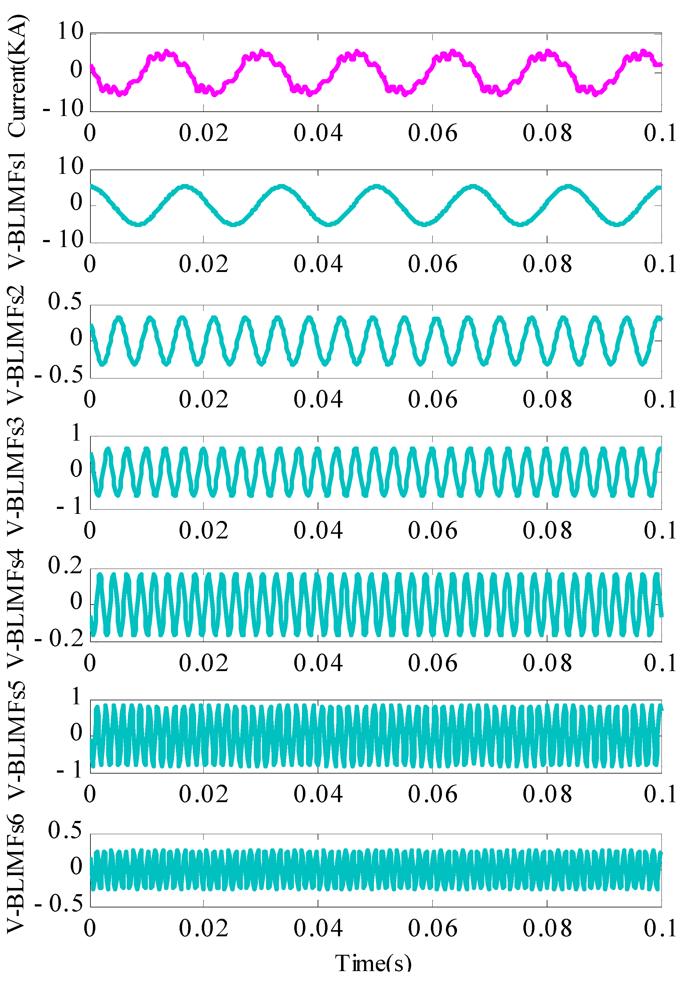
According to the determined modal decomposition number (K), the proposed algorithm is used to extract the harmonic parameters. The decomposition results are shown in Figure 8. The original signal contains six fixed and stable harmonic components decomposed by AVMD. Furthermore, HT is used to extract the harmonic parameters. The extracted harmonic parameters obtained by the AVMD, EMD, and FFT are provided in

Table 5. Harmonic detection results of measured current signal containing harmonics.

Algorithm	Harmonic	Frequency (Hz)	Amplitude (KA)	Phase (°)	Calculation Time (s)
AVMD + HT	Fundamental	59.0134	5.0320	0.2040	13.57
	3rd	179.9635	0.2937	35.8794
	5th	300.4672	0.8210	10.1359
	7th	419.3951	0.1435	89.9012
	11th	658.9123	0.6540	51.0432
	13th	781.8643	0.3028	1.2051
EMD + HT	Fundamental	59.3473	5.5027	0.34570	2.2
	5th	301.6321	0.9431	112.1425
	11th	660.3748	0.6031	50.2937
FFT	Fundamental	60.1538	1.536	-	0.7
	3rd	180.3241	0.1257	-
	5th	300.6412	0.2014	-
	7th	420.4689	0.06329	-
	11th	659.9677	0.185	-
	13th	780.1237	0.0985	-

. Meanwhile, the calculation time of the three detection algorithms are also listed in Table 5. As can be seen from Table 5, compared with the results of test signal, since more harmonic components contained in the measured data, the AVMD needs more calculation time, which is also far more than the other two methods.

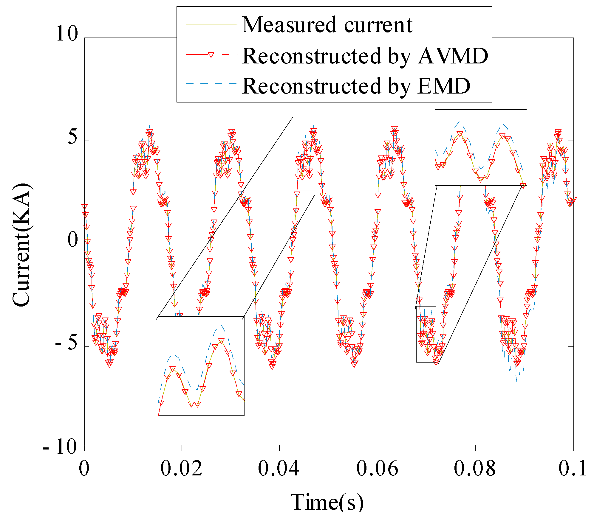
The harmonic parameters in Table 5 extracted using the AVMD and EMD algorithms are used to reconstruct the signals, and the results are shown in Figure 9. The signal reconstructed by the proposed method is better fitted to the original measured signal. Meanwhile, the calculation results of the SNR given in

Table 6. Calculation results for the SNR of the measured currents containing harmonics.

Algorithm	SNR (dB)
AVMD + HT	32.6327
EMD + HT	8.5714

indicate that the proposed method exhibits good superiority in harmonic parameter detection.

The above results show that the AVMD method consumes the longest calculation time, but the detection results have the best detection accuracy. The measured data analysis results further indicate that the AVMD method has better adaptability in power system harmonic detection.

With the continuous improvement of computer processing performance, the calculation time of the proposed method will not be significantly different from the other two methods, but the proposed method has the better detection accuracy. Therefore, the AVMD method has great advantages in power system harmonic detection.

5. Conclusions

In this study, the AVMD algorithm is used to analyze harmonic detection in power system, and the harmonic parameter extraction method based on the AVMD and HT is proposed. AVMD is a non-recursive algorithm. Harmonic signal detection is realized by constructing a constrained variational model and searching for the optimal solution. The analysis of the test signal and measured data shows that the proposed method is robust to noise, and the mode-mixing and false mode problems generated during the decomposition process of the EMD algorithm can be effectively avoided. The AVMD algorithm is highly adaptive to the harmonic parameter extraction of multi-harmonic coupled signals, and the parameter detection results can accurately reflect harmonic characteristics.

The proposed method provides a powerful analysis tool for harmonic characteristic parameter extraction in power system.