Daily Natural Gas Load Forecasting Based on a Hybrid Deep Learning Model

Abstract
:1. Introduction
- (a)
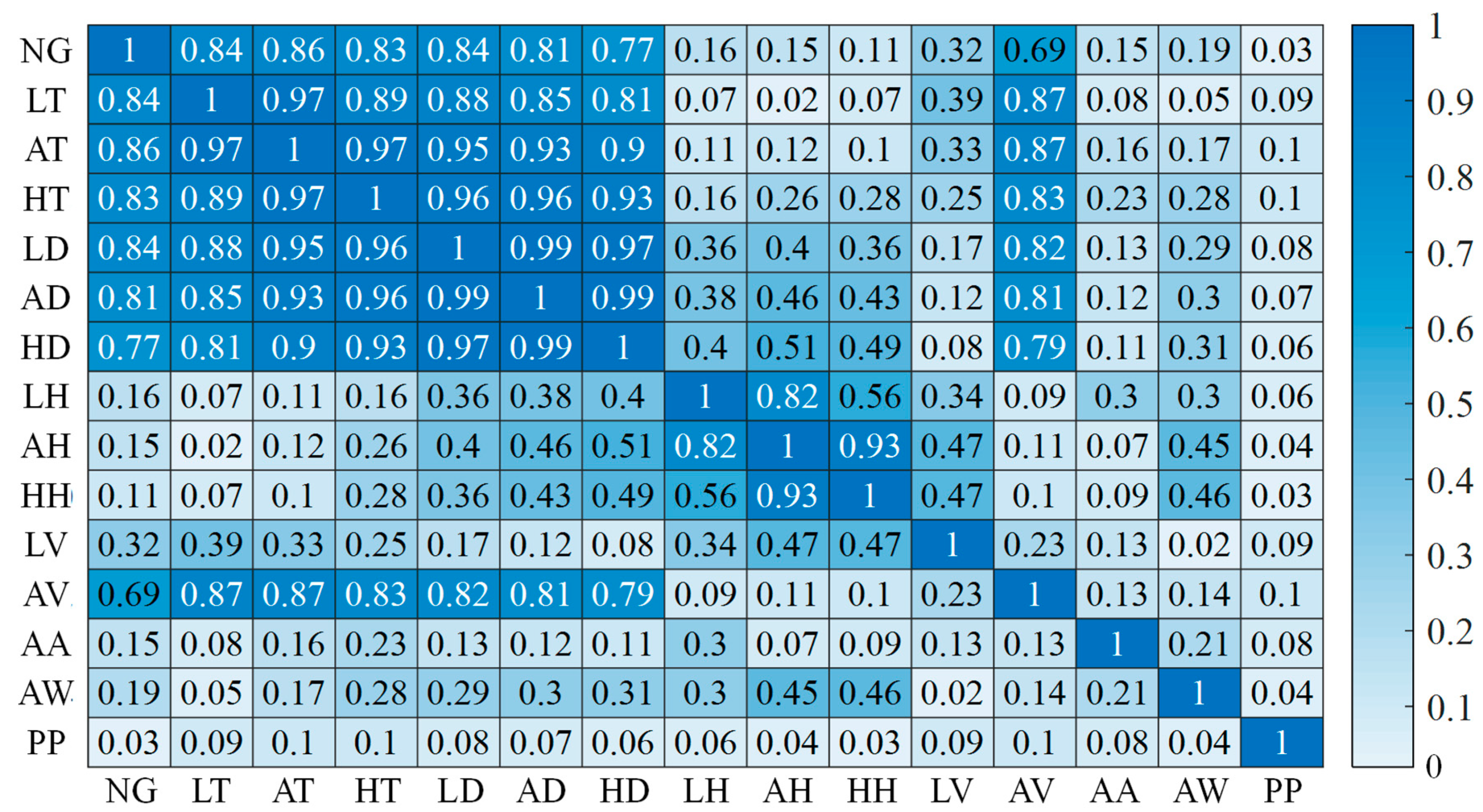
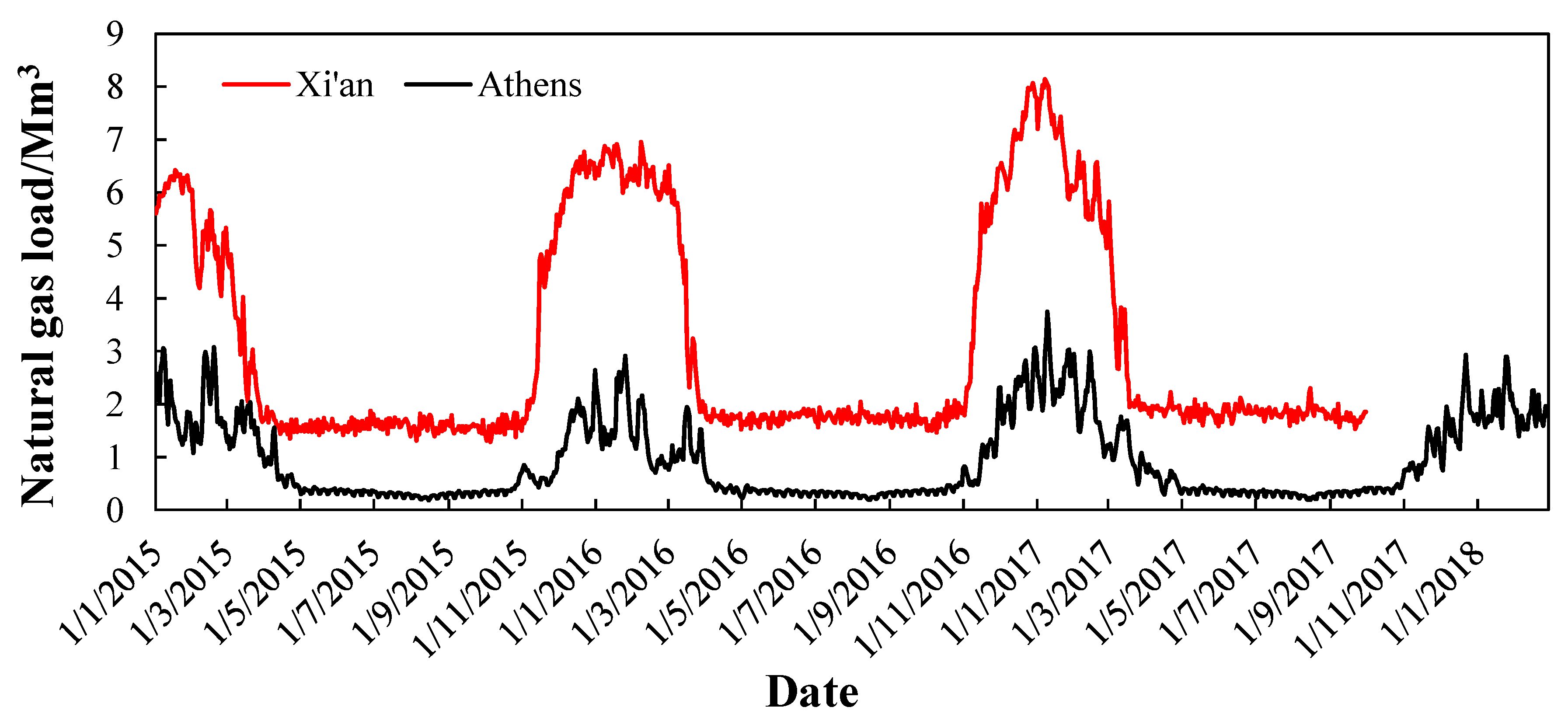
- This paper is mainly concerned with the recent data of Xi’an (China) and Athens (Greece). Contrary to the majority of the literature that focuses on the NGLF of cities in a certain country or area, this paper aims to develop a robust and feasible model to provide an accurate NGLF of cities worldwide. Using case studies, over two years of data on the natural gas load and 14 weather variations were used to validate the performance of the proposed model.
- (b)
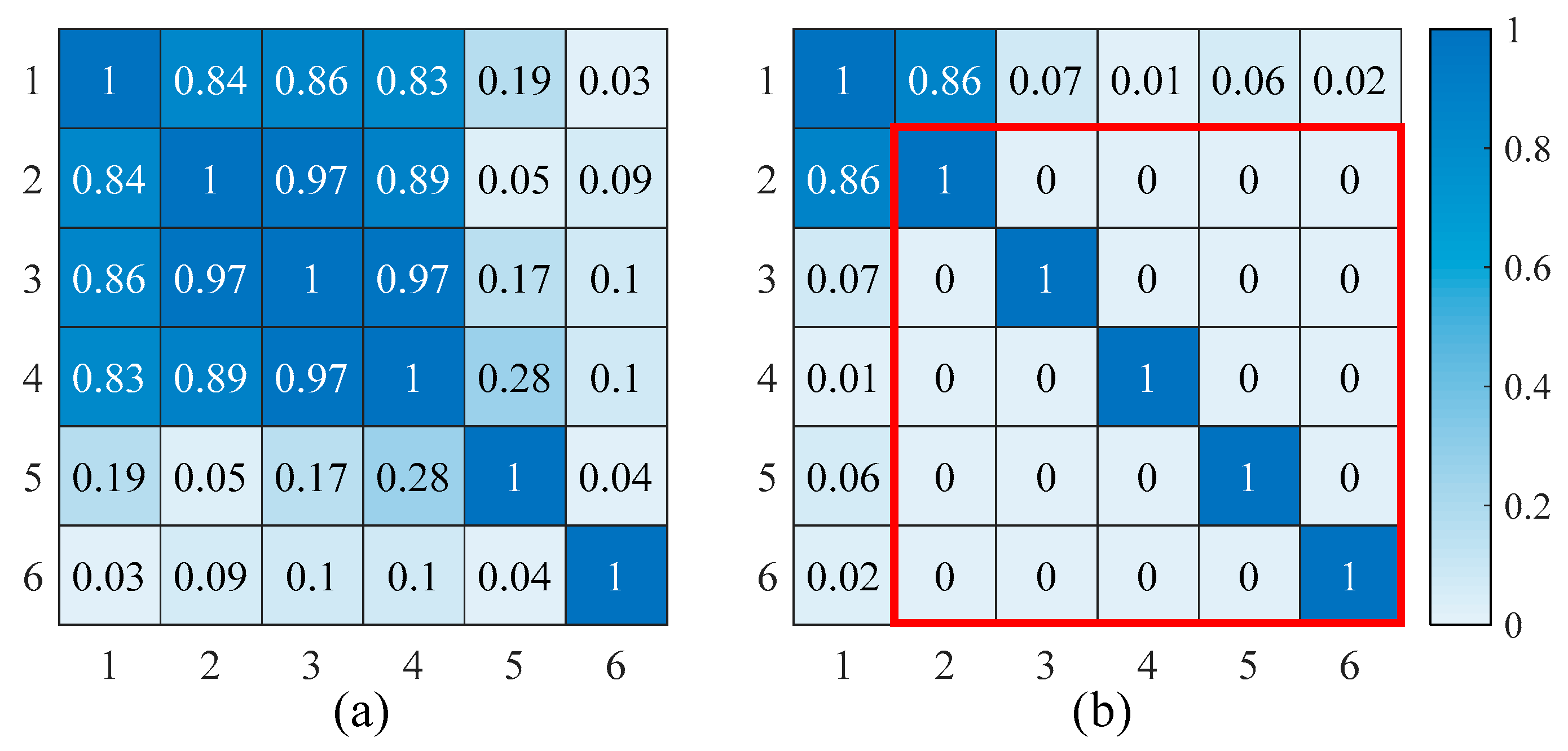
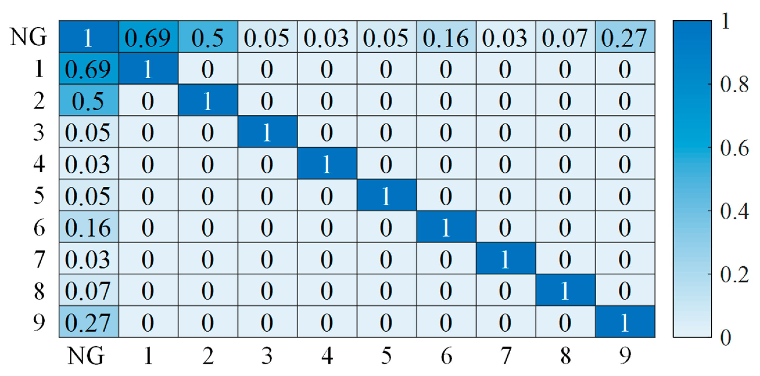
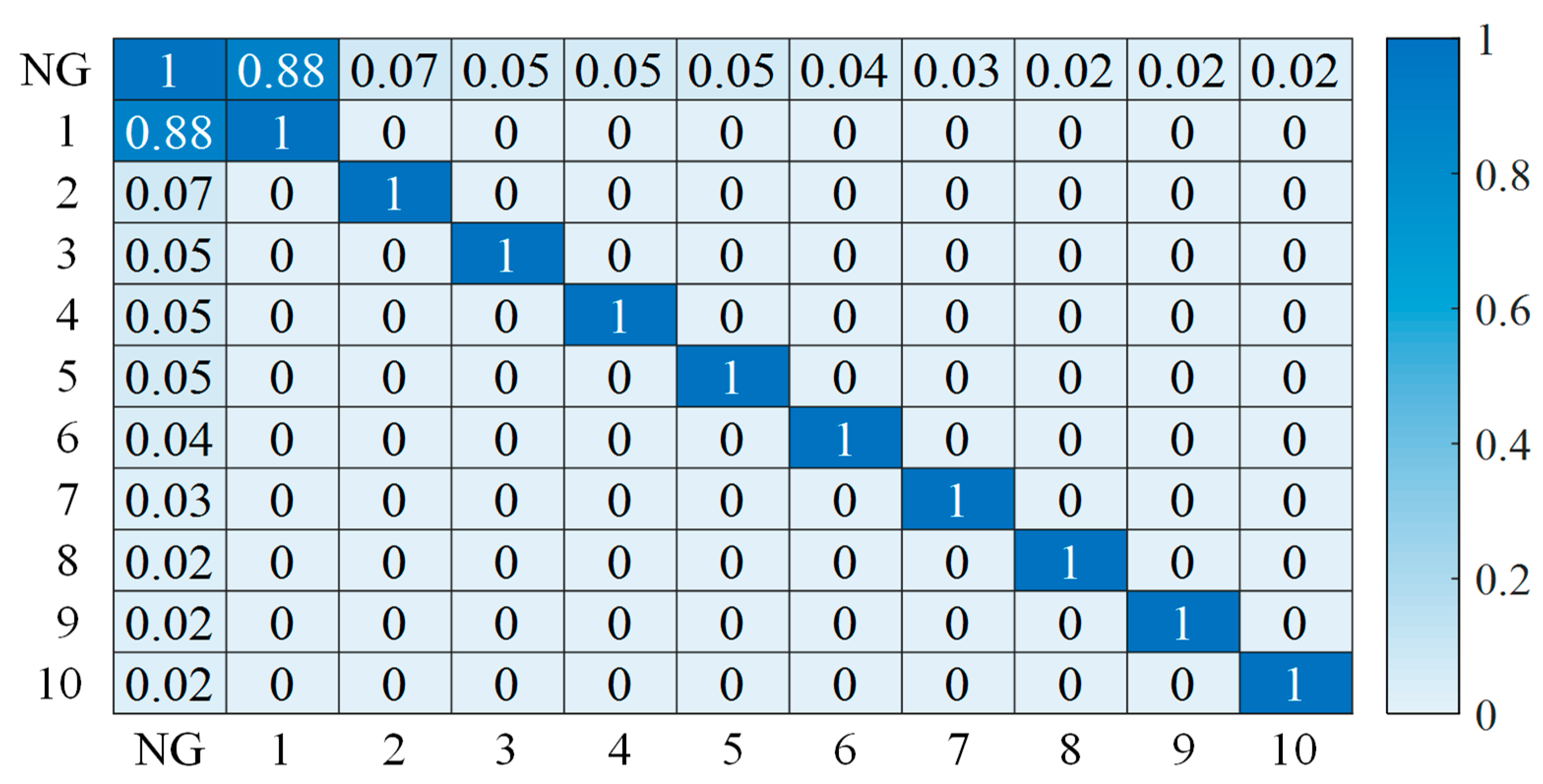
- PCCA is first proposed in this paper. With PCCA, we developed a novel selection mechanism which considers correlation between each component in the eigenspace to select proper candidates for the input dataset of the forecasting model. This method can not only reduce the dimension of the input dataset but also automatically remove the redundant components.
- (c)
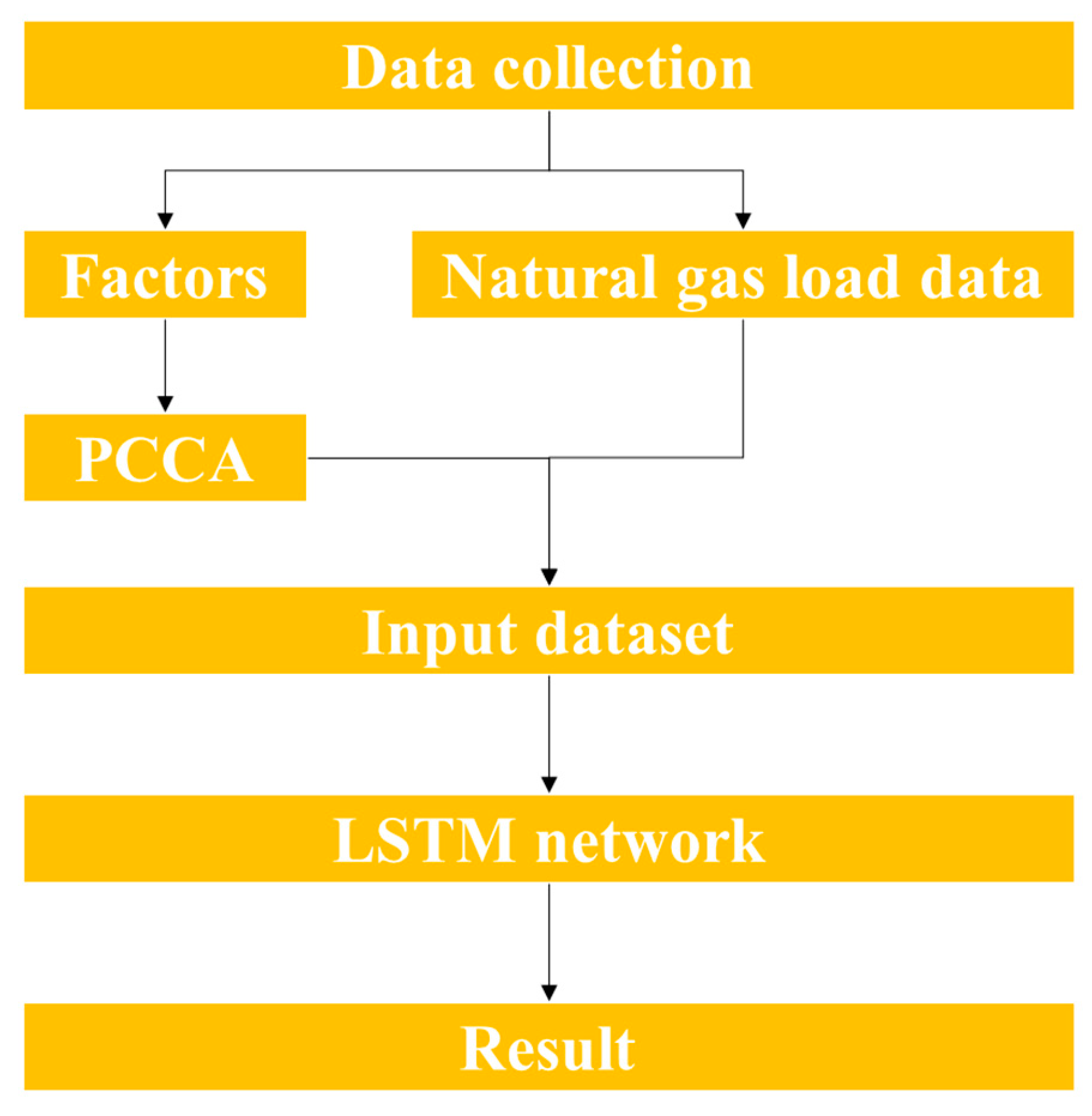
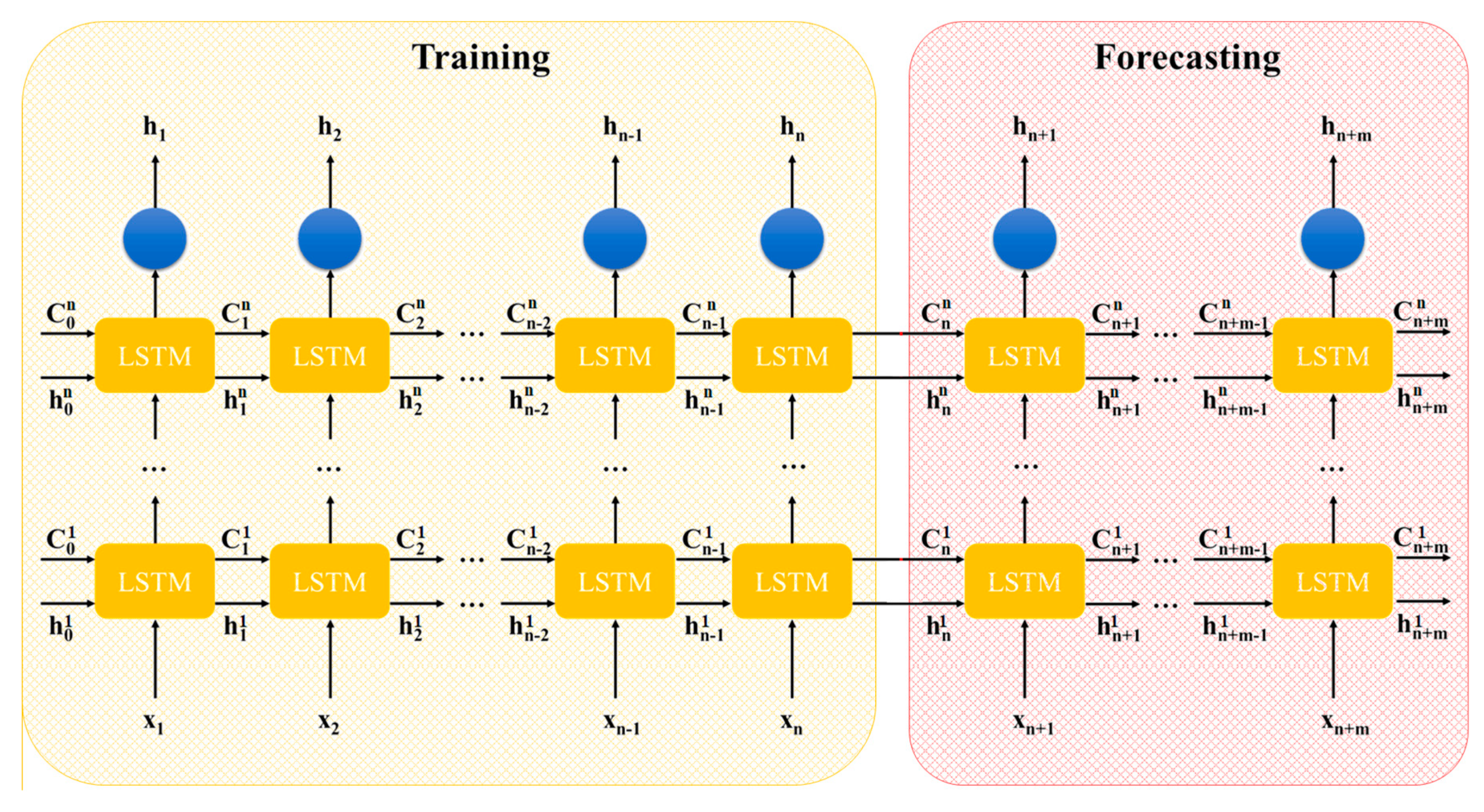
- A hybrid DL-based model is proposed for NGLF. This hybrid model combines PCCA and the LSTM network and is referred to as PCCA–LSTM. Practically, PCCA was used to remove redundant components and LSTM was applied to predict the natural gas load of cities in China and Greece. In addition, the comparative performance analysis of PCCA–LSTM with BPNN-, LSTM-, and SVR-based models is shown in this paper.
2. Natural Gas Load Forecasting Framework
2.1. Principal Component Correlation Analysis
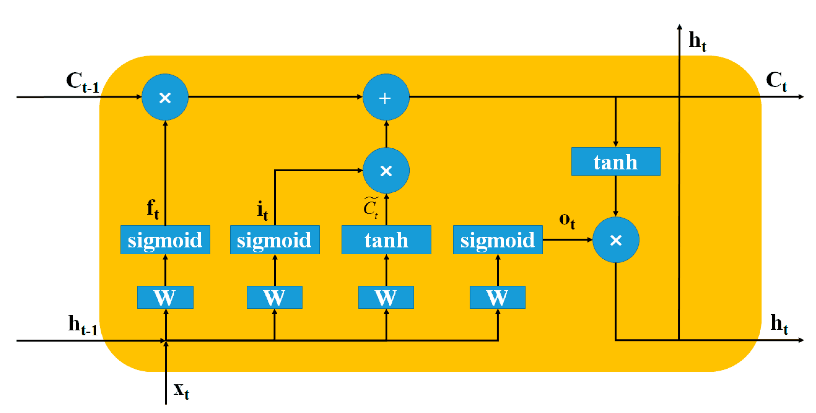
2.2. Long Short-Term Memory
2.3. Construction of the Hybrid Model: PCCA–LSTM
3. Case Studies
3.1. Evaluation Framework
3.2. Data Description
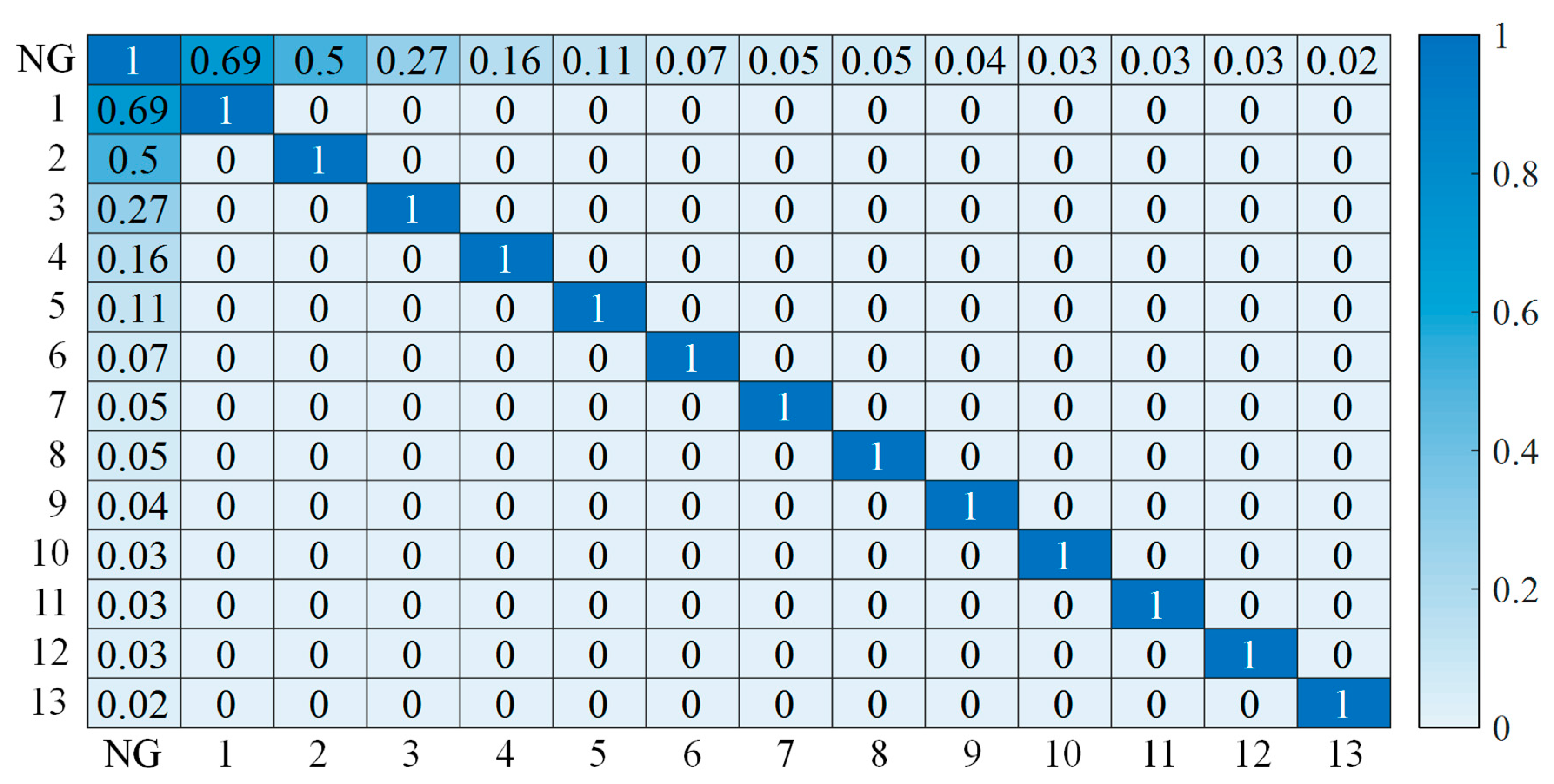
3.3. Xi’an Case
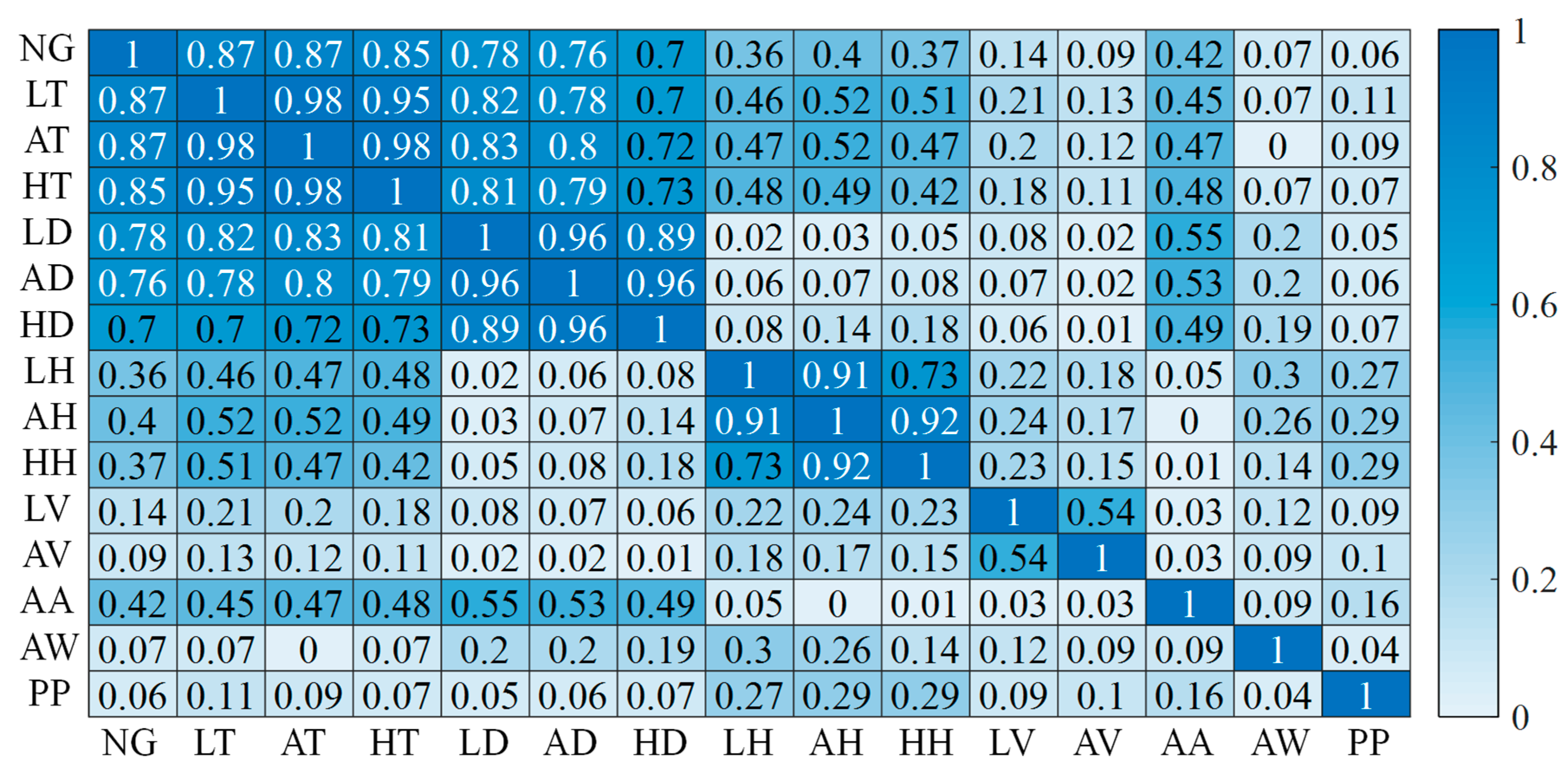
3.4. Athens Case
4. Conclusions
Author Contributions
Funding
Conflicts of Interest
References
- Bunn, D.W. Short-term forecasting: A review of procedures in the electricity supply industry. J. Oper. Res. Soc. 1982, 33, 533–545. [Google Scholar] [CrossRef]
- Tamba, J.G.; Essiane, S.N.; Sapnken, E.F.; Koffi, F.D.; Nsouandélé, J.L.; Soldo, B.; Njomo, D. Forecasting Natural Gas: A Literature Survey. Int. J. Energy Econ. Policy 2018, 8, 216–249. [Google Scholar]
- Natgas Natural Gas Demand. Available online: http://naturalgas.org/business/demand/#factorshort (accessed on 20 September 2013).
- DESFA Historical Data of Natural Gas Deliveries. Available online: http://www.desfa.gr/en/regulatory-services (accessed on 1 March 2018).
- Soldo, B. Forecasting natural gas consumption. Appl. Energy 2012, 92, 26–37. [Google Scholar] [CrossRef]
- Wei, N.; Li, C.; Li, C.; Xie, H.; Du, Z.; Zhang, Q.; Zeng, F. Short-term forecasting of natural gas consumption using factor selection algorithm and optimized support vector regression. J. Energy Resour. Technol. 2018, 141, 032701. [Google Scholar] [CrossRef]
- Hubbert, M. Nuclear Energy and the Fossil Fuel. In Drilling and Production Practice; American Petroleum Institute: Washington, DC, USA, 1956. [Google Scholar]
- Wang, J.; Jiang, H.; Zhou, Q.; Wu, J.; Qin, S. China’s natural gas production and consumption analysis based on the multicycle Hubbert model and rolling Grey model. Renew. Sustain. Energy Rev. 2016, 53, 1149–1167. [Google Scholar] [CrossRef]
- Ediger, V.Ş.; Akar, S. ARIMA forecasting of primary energy demand by fuel in Turkey. Energy Policy 2007, 35, 1701–1708. [Google Scholar] [CrossRef]
- Brown, R.H.; Matin, I. Development of artificial neural network models to predict daily gas consumption. In Proceedings of the IEEE IECON 21st International Conference on Industrial Electronics, Control, and Instrumentation, Orlando, FL, USA, 6–10 November 1995; Volume 2, pp. 1389–1394. [Google Scholar]
- Bai, Y.; Li, C. Daily natural gas consumption forecasting based on a structure-calibrated support vector regression approach. Energy Build. 2016, 127, 571–579. [Google Scholar] [CrossRef]
- Lee, Y.S.; Tong, L.I. Forecasting time series using a methodology based on autoregressive integrated moving average and genetic programming. Knowl. Based Syst. 2011, 24, 66–72. [Google Scholar] [CrossRef]
- Kaynar, O.; Yilmaz, I.; Demirkoparan, F. Forecasting of natural gas consumption with neural network and neuro fuzzy system. In Proceedings of the EGU General Assembly Conference, Vienna, Austria, 2–7 May 2010; pp. 221–238. [Google Scholar]
- Divina, F.; Gilson, A.; Goméz-Vela, F.; García Torres, M.; Torres, J.F. Stacking Ensemble Learning for Short-Term Electricity Consumption Forecasting. Energies 2018, 11, 949. [Google Scholar] [CrossRef]
- Zhou, X.; Yuan, Q.; Rui, Z.; Wang, H.; Feng, J.; Zhang, L.; Zeng, F. Feasibility study of CO2 huff’n’puff process to enhance heavy oil recovery via long core experiments. Appl. Energy 2019, 236, 526–539. [Google Scholar] [CrossRef]
- Yu, F.; Xu, X. A short-term load forecasting model of natural gas based on optimized genetic algorithm and improved BP neural network. Appl. Energy 2014, 134, 102–113. [Google Scholar] [CrossRef]
- Zhu, L.; Li, M.; Wu, Q.; Jiang, L. Short-term natural gas demand prediction based on support vector regression with false neighbours filtered. Energy 2015, 80, 428–436. [Google Scholar] [CrossRef]
- He, Y.; Liu, R.; Li, H.; Wang, S.; Lu, X. Short-term power load probability density forecasting method using kernel-based support vector quantile regression and Copula theory. Appl. Energy 2017, 185, 254–266. [Google Scholar] [CrossRef]
- Zhang, X.; Wang, J.; Zhang, K. Short-term electric load forecasting based on singular spectrum analysis and support vector machine optimized by Cuckoo search algorithm. Electr. Power Syst. Res. 2017, 146, 270–285. [Google Scholar] [CrossRef]
- Chen, H.; Engkvist, O.; Wang, Y.; Olivecrona, M.; Blaschke, T. The rise of deep learning in drug discovery. Drug Discov. Today 2018, 23, 1241–1250. [Google Scholar] [CrossRef] [PubMed]
- Ghasemi, F.; Mehridehnavi, A.; Fassihi, A.; Pérez-Sánchez, H. Deep neural network in QSAR studies using deep belief network. Appl. Soft Comput. 2018, 62, 251–258. [Google Scholar] [CrossRef]
- Krizhevsky, A.; Sutskever, I.; Hinton, G.E. ImageNet classification with deep convolutional neural networks. In Proceedings of the 25th International Conference on Neural Information Processing Systems—Volume 1, Lake Tahoe, NV, USA; 2012; pp. 1097–1105. [Google Scholar]
- Graves, A. Supervised Sequence Labelling with Recurrent Neural Networks; Springer: Berlin/Heidelberg, Germany, 2012. [Google Scholar]
- He, W. Load Forecasting via Deep Neural Networks. Procedia Comput. Sci. 2017, 122, 308–314. [Google Scholar] [CrossRef]
- Gensler, A.; Henze, J.; Sick, B.; Raabe, N. Deep Learning for solar power forecasting—An approach using AutoEncoder and LSTM Neural Networks. In Proceedings of the IEEE International Conference on Systems, Man, and Cybernetics, Banff, Canada, 5–8 October 2017; pp. 002858–002865. [Google Scholar]
- Zaytar, M.A.; El Amrani, C. Sequence to sequence weather forecasting with long short term memory recurrent neural networks. Int. J. Comput. Appl. 2016, 143, 7–11. [Google Scholar]
- Zhou, X.; Yuan, Q.; Zhang, Y.; Wang, H.; Zeng, F.; Zhang, L. Performance evaluation of CO2 flooding process in tight oil reservoir via experimental and numerical simulation studies. Fuel 2019, 236, 730–746. [Google Scholar] [CrossRef]
- Malvoni, M.; Giorgi, M.G.D.; Congedo, P.M. Photovoltaic forecast based on hybrid PCA–LSSVM using dimensionality reducted data. Neurocomputing 2016, 211, 72–83. [Google Scholar] [CrossRef]
- Bianchi, F.M.; Santis, E.D.; Rizzi, A.; Sadeghian, A. Short-Term Electric Load Forecasting Using Echo State Networks and PCA Decomposition. IEEE Access 2015, 3, 1931–1943. [Google Scholar] [CrossRef]
- Lecun, Y.; Bengio, Y.; Hinton, G. Deep learning. Nature 2015, 521, 436. [Google Scholar] [CrossRef] [PubMed]
- Jolliffe, I.T. Principal component analysis. J. Mark. Res. 2002, 87, 513. [Google Scholar]
- Li, B.; Morris, J.; Martin, E.B. Model selection for partial least squares regression. Chemom. Intell. Lab. Syst. 2002, 64, 79–89. [Google Scholar] [CrossRef]
- Harrou, F.; Kadri, F.; Chaabane, S.; Tahon, C.; Sun, Y. Improved principal component analysis for anomaly detection: Application to an emergency department. Comput. Ind. Eng. 2015, 88, 63–77. [Google Scholar] [CrossRef]
- Zhu, M.; Ghodsi, A. Automatic dimensionality selection from the scree plot via the use of profile likelihood. Comput. Stat. Data Anal. 2006, 51, 918–930. [Google Scholar] [CrossRef]
- White, D.A.; Goodlin, B.E.; Gower, A.E.; Boning, D.S.; Chen, H.; Sawin, H.H.; Dalton, T.J. Low open-area endpoint detection using a PCA-based T/sup 2/statistic and Q statistic on optical emission spectroscopy measurements. IEEE Trans. Semicond. Manuf. 2002, 13, 193–207. [Google Scholar] [CrossRef]
- Taylor, R. Interpretation of the correlation coefficient: A basic review. J. Diagn. Med. Sonogr. 1990, 6, 35–39. [Google Scholar] [CrossRef]
- Zhao, Z.; Chen, W.; Wu, X.; Chen, P.C.Y.; Liu, J. LSTM network: A deep learning approach for short-term traffic forecast. IET Intell. Transp. Syst. 2017, 11, 68–75. [Google Scholar] [CrossRef]
- Zheng, H.; Yuan, J.; Chen, L. Short-Term Load Forecasting Using EMD-LSTM Neural Networks with a Xgboost Algorithm for Feature Importance Evaluation. Energies 2017, 10, 1168. [Google Scholar] [CrossRef]
- Panapakidis, I.P.; Dagoumas, A.S. Day-ahead natural gas demand forecasting based on the combination of wavelet transform and ANFIS/genetic algorithm/neural network model. Energy 2017, 118, 231–245. [Google Scholar] [CrossRef]
- Lewis, C. Industrial and Business Forecasting Methods: A Practical Guide to Exponential Smoothing and Curve Fitting; Butterworth Scientific: London, UK, 1982. [Google Scholar]
- OECD. OECD Urban Policy Reviews: China 2015; OECD: Paris, France, 2015. [Google Scholar] [CrossRef]
- Nations, U. Greece Population. Available online: http://worldpopulationreview.com/countries/greece-population (accessed on 24 September 2018).
- Wright, C.; Chan, C.W.; Laforge, P. Towards Developing a Decision Support System for Electricity Load Forecast. Available online: https://www.intechopen.com/books/decision-support-systems_2012/towards-developing-a-decision-support-system-for-electricity-load-forecast (accessed on 17 October 2012).


| MAPE | ≤10% | 10%–20% | 20%–50% | ≥50% |
|---|---|---|---|---|
| Evaluation | Highly accurate | Good | Reasonable | Inaccurate |
| City | Training | Testing | ||
|---|---|---|---|---|
| Data | Length | Data | Length | |
| Xi’an | 1 January 2015 to 31 August 2017 | 974 | 1–30 September 2017 | 30 |
| Athens | 1 January 2015 to 31 December 2017 | 1096 | 1 January 2018 to 28 Feburary 2018 | 59 |
| Items | BPNN | GA-SVR | LSTM | PCA–LSTM | PCCA–LSTM |
|---|---|---|---|---|---|
| Time (s) | 155.77 | 241.23 | 186.34 | 110.07 | 162.31 |
| MAE | 0.17 | 0.15 | 0.10 | 0.11 | 0.06 |
| RMSE | 0.04 | 0.03 | 0.03 | 0.03 | 0.01 |
| MARNE | 9.32% | 7.98% | 5.87% | 6.03% | 3.02% |
| MAPE | 10.04% | 8.23% | 6.56% | 6.99% | 3.22% |
| Evaluation | Good | Highly accurate | Highly accurate | Highly accurate | Highly accurate |
| Items | BPNN | GA-SVR | LSTM | PCA–LSTM | PCCA–LSTM |
|---|---|---|---|---|---|
| Time(s) | 176.39 | 303.01 | 154.34 | 106.07 | 139.31 |
| MAE | 0.29 | 0.3 | 0.14 | 0.26 | 0.13 |
| RMSE | 0.1 | 0.09 | 0.04 | 0.07 | 0.04 |
| MARNE | 14.02% | 14.19% | 5.56% | 11.27% | 6.66% |
| MAPE | 16.53% | 17.14% | 7.88% | 13.40% | 7.29% |
| Evaluation | Good | Good | Highly accurate | Good | Highly accurate |
© 2019 by the authors. Licensee MDPI, Basel, Switzerland. This article is an open access article distributed under the terms and conditions of the Creative Commons Attribution (CC BY) license (http://creativecommons.org/licenses/by/4.0/).
Share and Cite
Wei, N.; Li, C.; Duan, J.; Liu, J.; Zeng, F. Daily Natural Gas Load Forecasting Based on a Hybrid Deep Learning Model. Energies 2019, 12, 218. https://doi.org/10.3390/en12020218
Wei N, Li C, Duan J, Liu J, Zeng F. Daily Natural Gas Load Forecasting Based on a Hybrid Deep Learning Model. Energies. 2019; 12(2):218. https://doi.org/10.3390/en12020218
Chicago/Turabian StyleWei, Nan, Changjun Li, Jiehao Duan, Jinyuan Liu, and Fanhua Zeng. 2019. "Daily Natural Gas Load Forecasting Based on a Hybrid Deep Learning Model" Energies 12, no. 2: 218. https://doi.org/10.3390/en12020218
APA StyleWei, N., Li, C., Duan, J., Liu, J., & Zeng, F. (2019). Daily Natural Gas Load Forecasting Based on a Hybrid Deep Learning Model. Energies, 12(2), 218. https://doi.org/10.3390/en12020218