Risk Assessment and Its Visualization of Power Tower under Typhoon Disaster Based on Machine Learning Algorithms


 ,
,
Abstract
1. Introduction
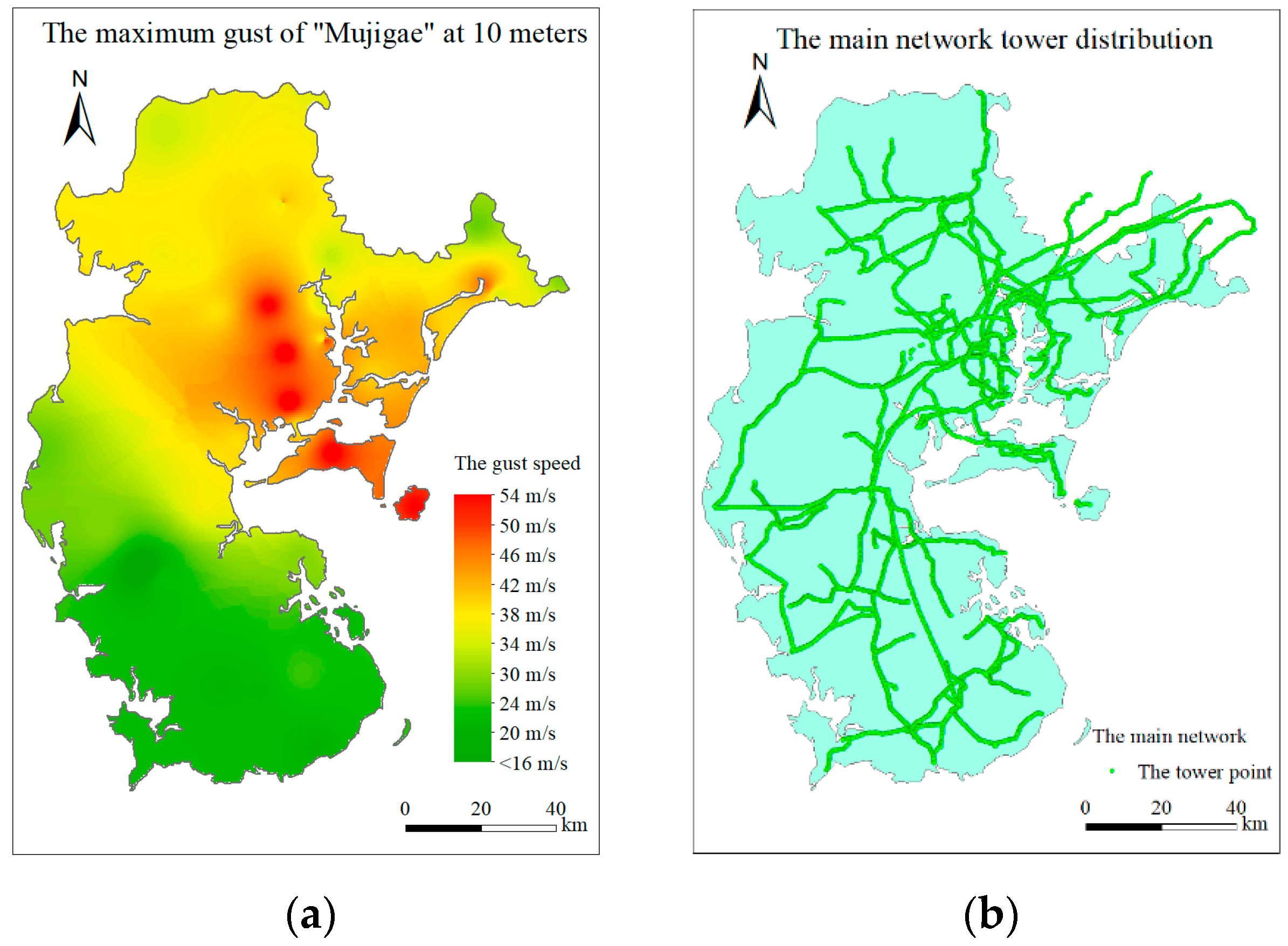
2. Study Area
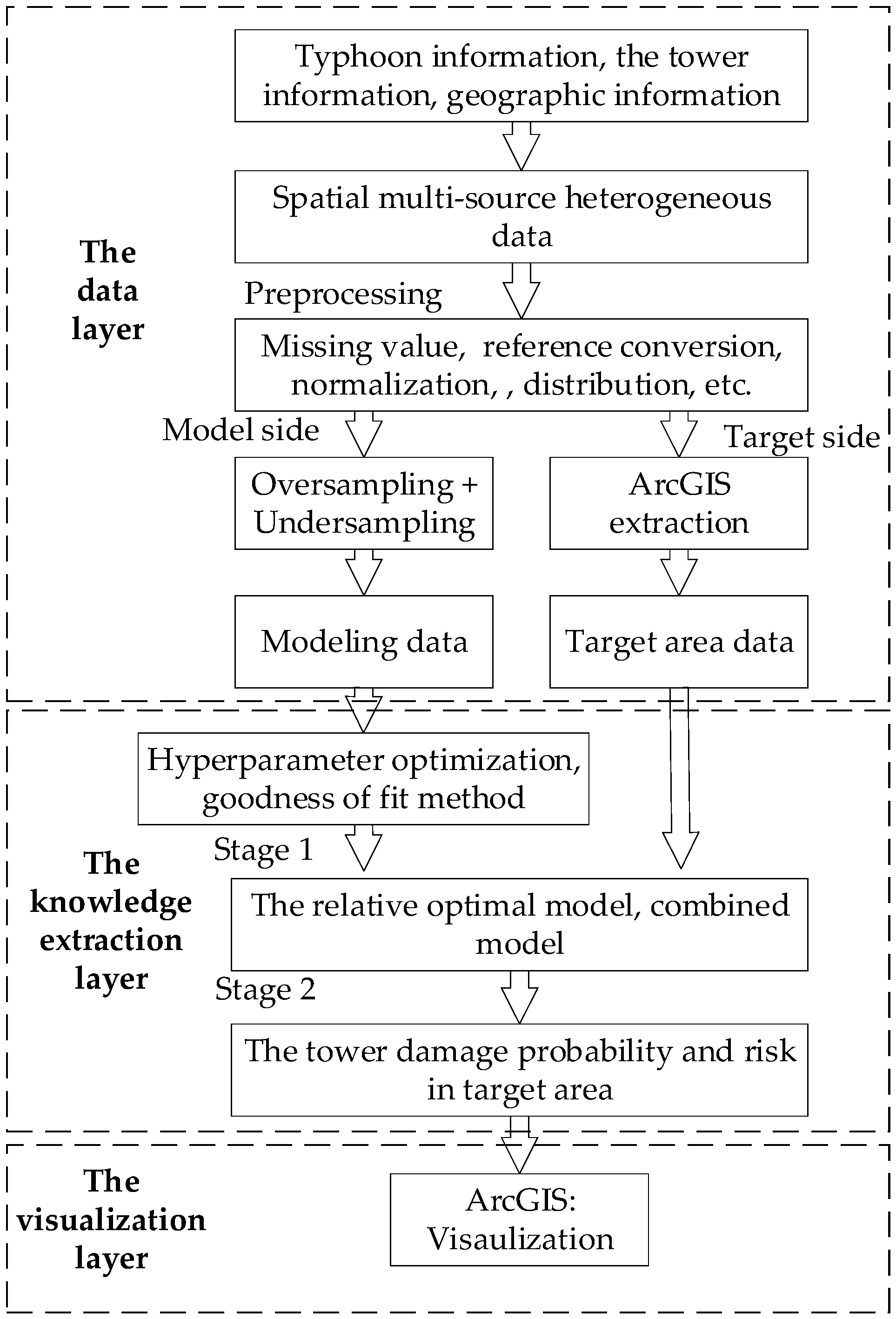
3. Framework for Risk Assessment and Its Visualization
4. Construction of Power Tower Risk Assessment System
4.1. Data Layer
4.1.1. Data Preprocessing
4.1.2. Processing of Model Side Data
4.1.3. Processing of Target Side Data
- Geographically mesh (rectangular grid constructed with latitude and longitude lines, hereinafter referred to as grid) the target area.
- Covert the maximum gust to 10 m high by method in Section 4.1.1 at each monitoring station under a typhoon, and the gust map is generated by the inverse distance weight interpolation method [22,23], and Vi,10 (the maximum gust at 10 m) in each grid is extracted, where i (i = 1,2,…, n) represents the grid serial number.
- Load the coordinates of the main network tower in the target area by ArcGIS 10.4, and extract Ni (the total number of towers), Vi,10 (design wind speed) from grid i.
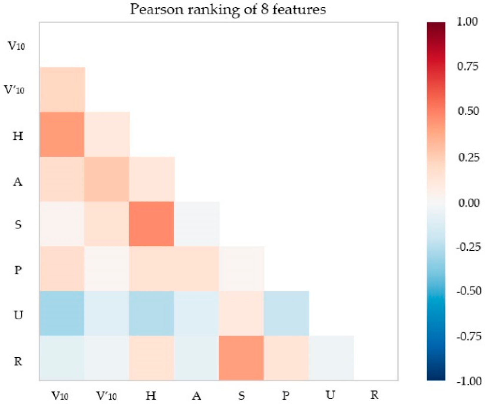
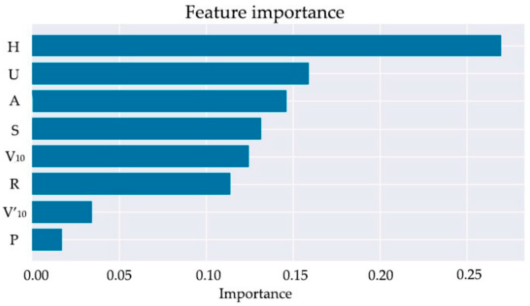
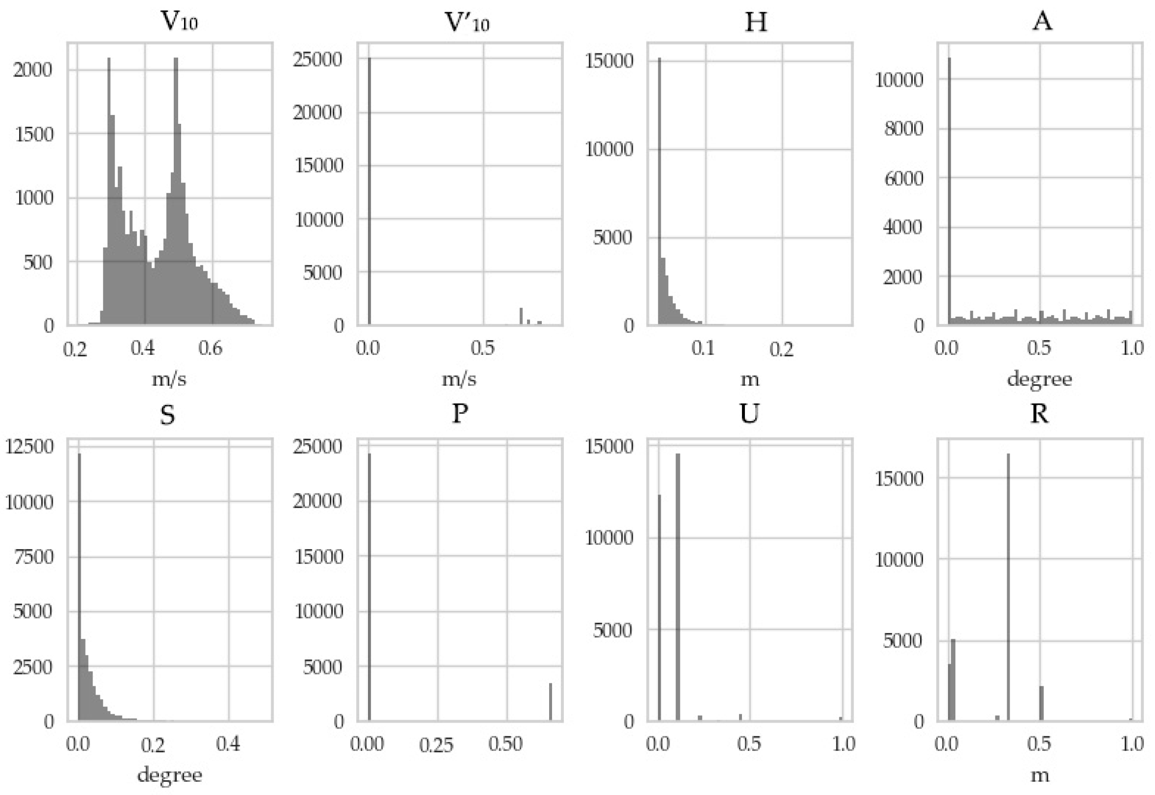
- Extract geographic information within the grid, including Hi, Ai, Si, Pi, Ui, Ri, and so on.
4.2. Knowledge Extraction Layer
4.2.1. Introduction to Algorithms
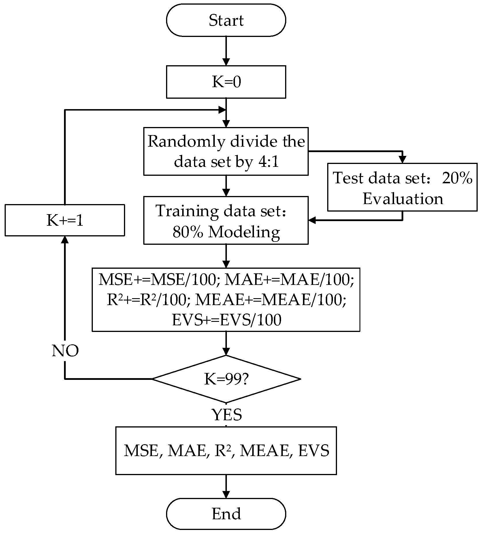
4.2.2. Single Intelligent Model
4.2.3. Combined Model
4.3. Visualization Layer
5. Materials and Methods
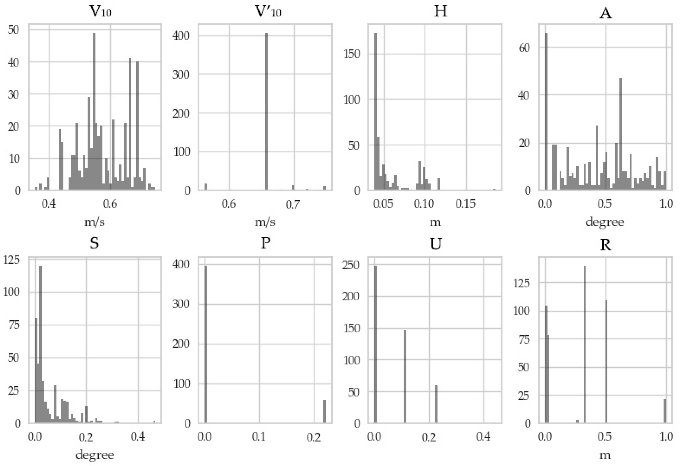
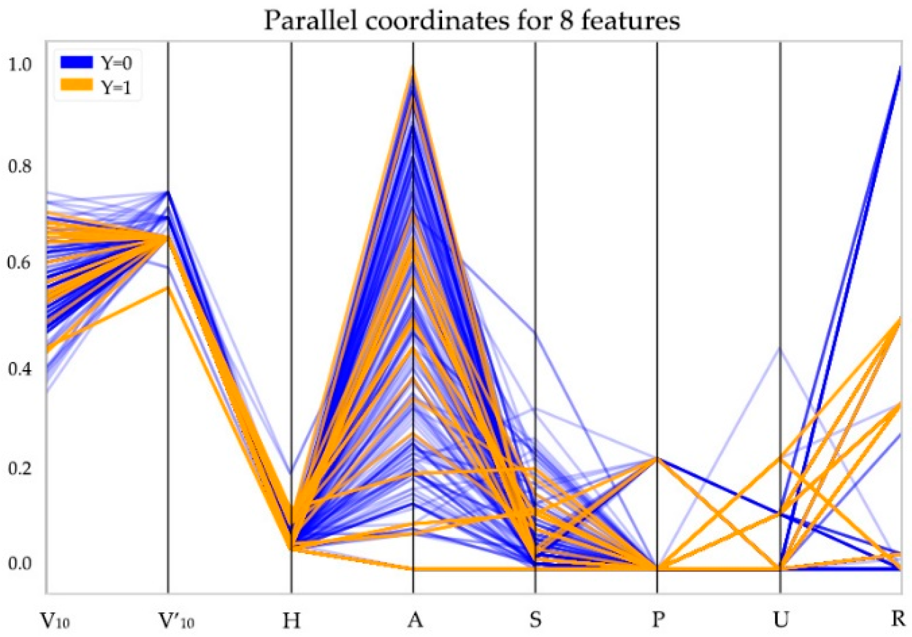
5.1. Processing of Model Side Data
5.2. Processing of Target Side Data
6. Results
6.1. Knowledge Extraction Layer
6.1.1. Single Intelligent Model
6.1.2. Combined Model
6.2. Visualization Layer
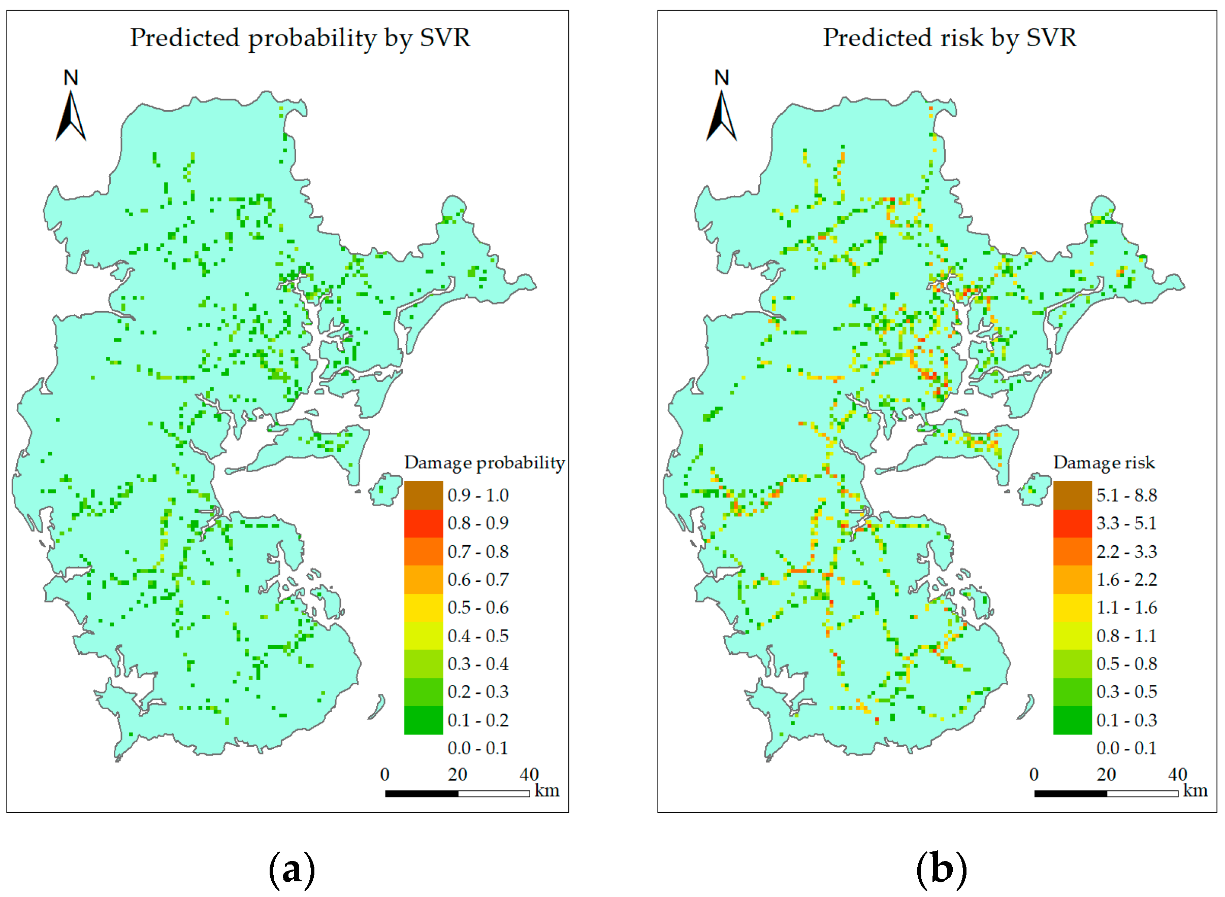
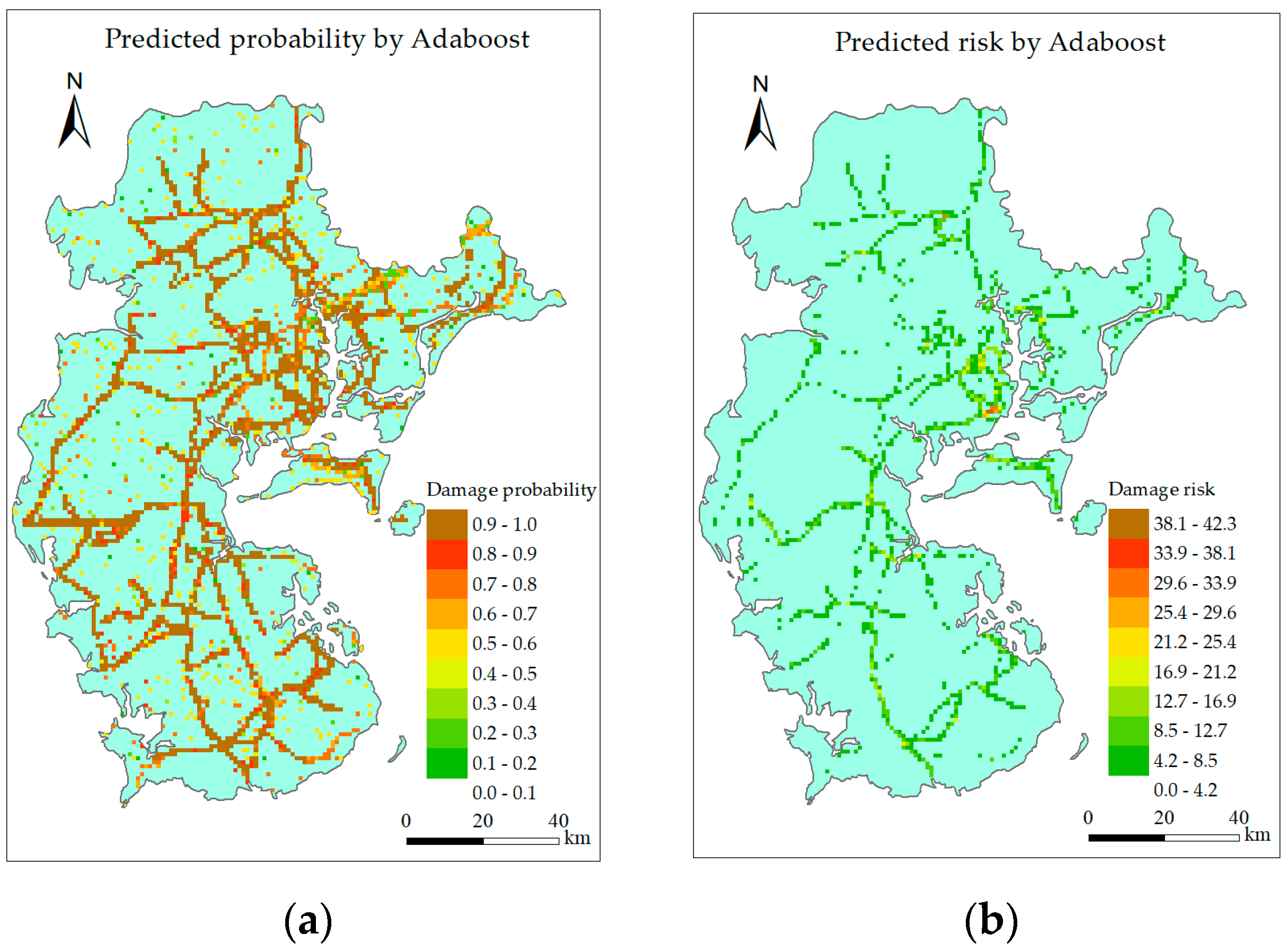
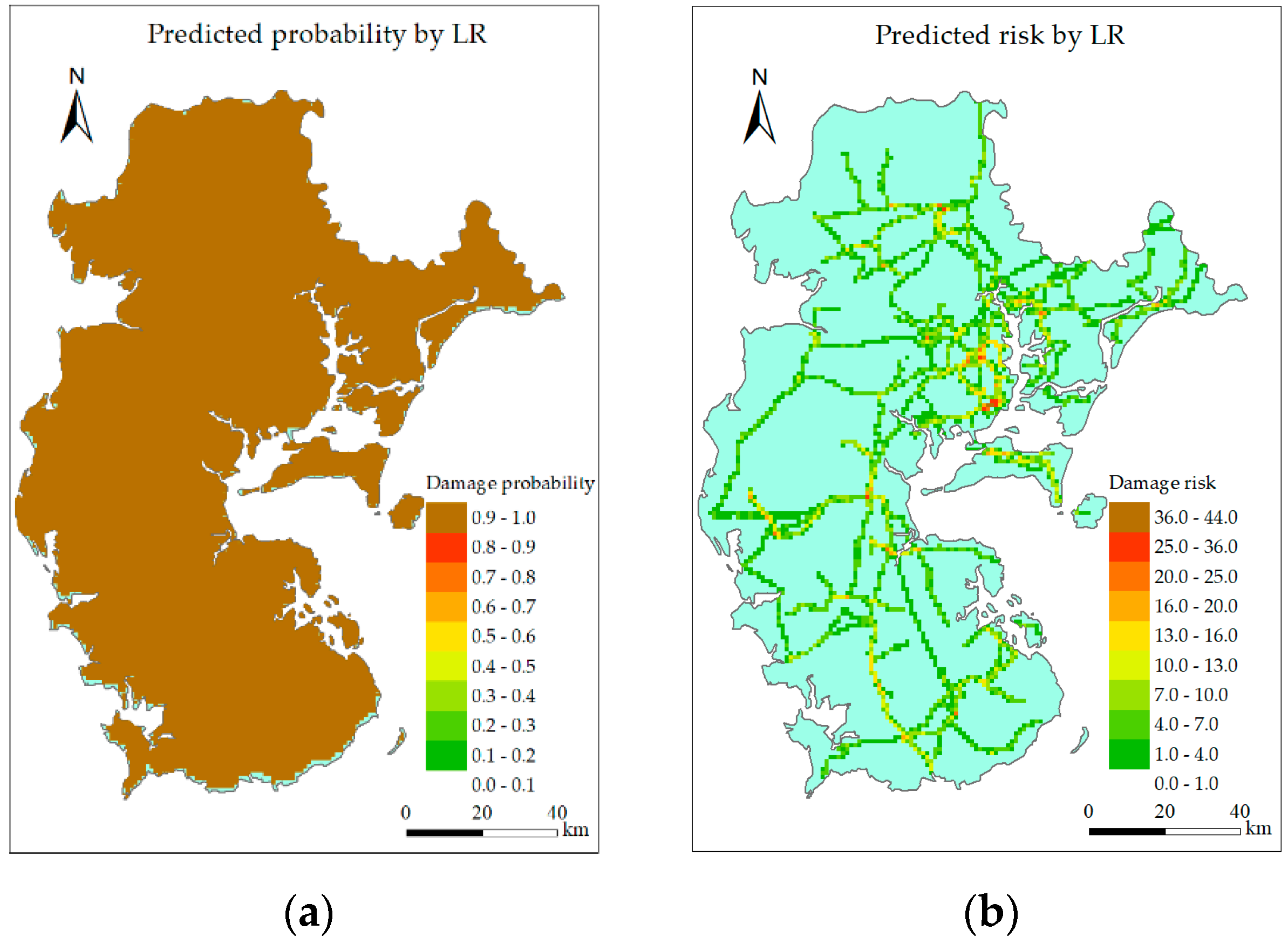
6.2.1. Single Intelligent Model
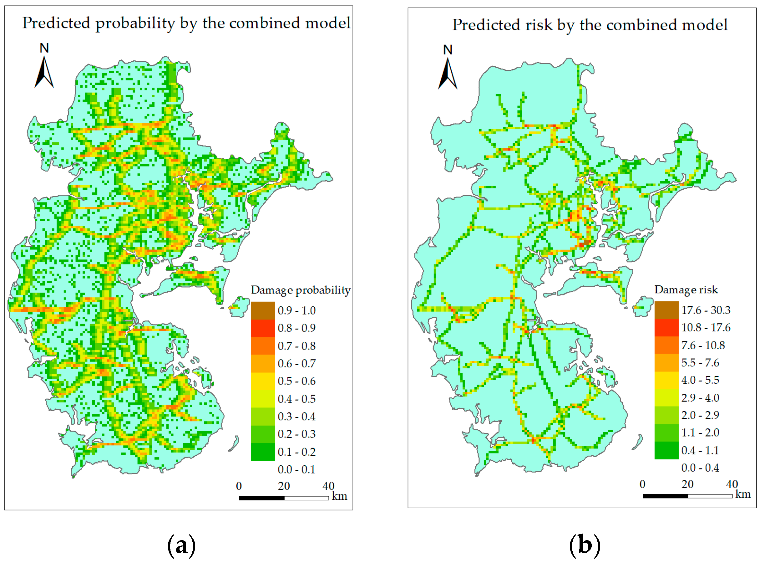
6.2.2. Combined Model
6.2.3. Discussion
7. Conclusions
- (1)
- (2)
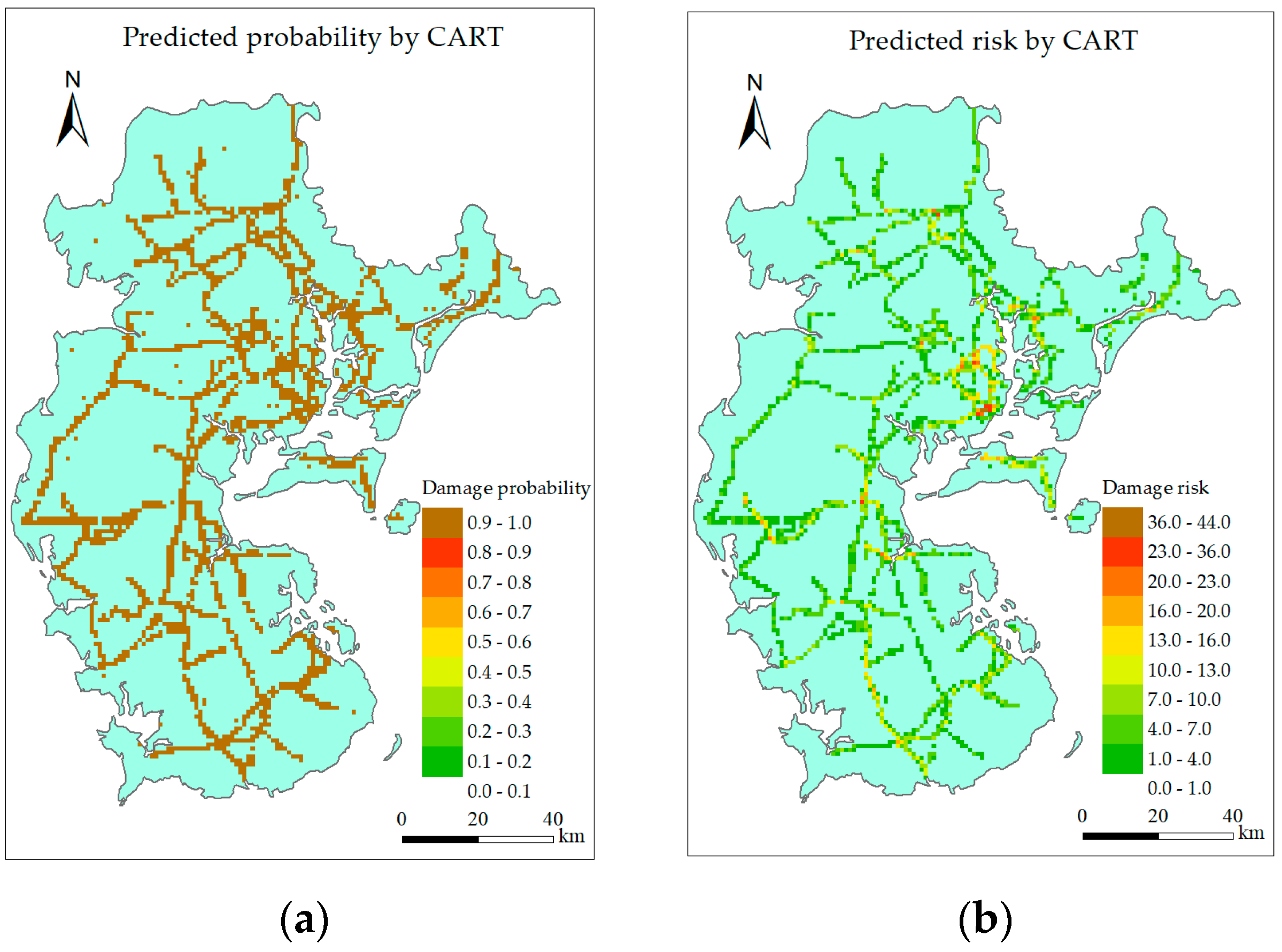
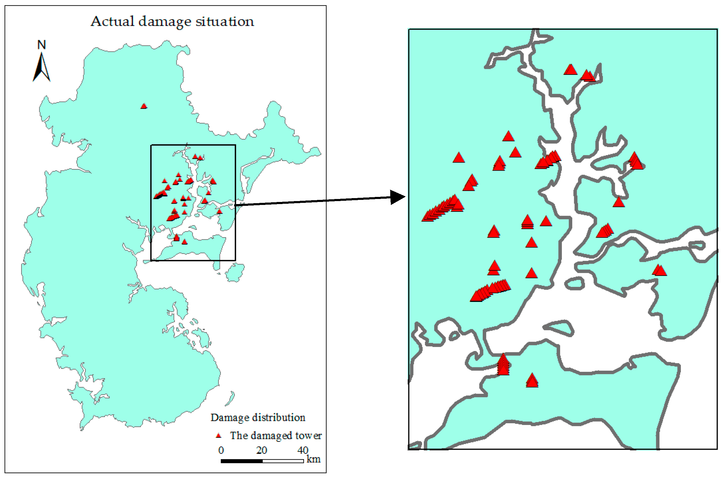
- Both the single intelligent model and combined model can identify the high-risk grids, but the combined model can reduce the predicting error at the low gust area while maintain the predicting accuracy around landing point and along typhoon track.
- (3)
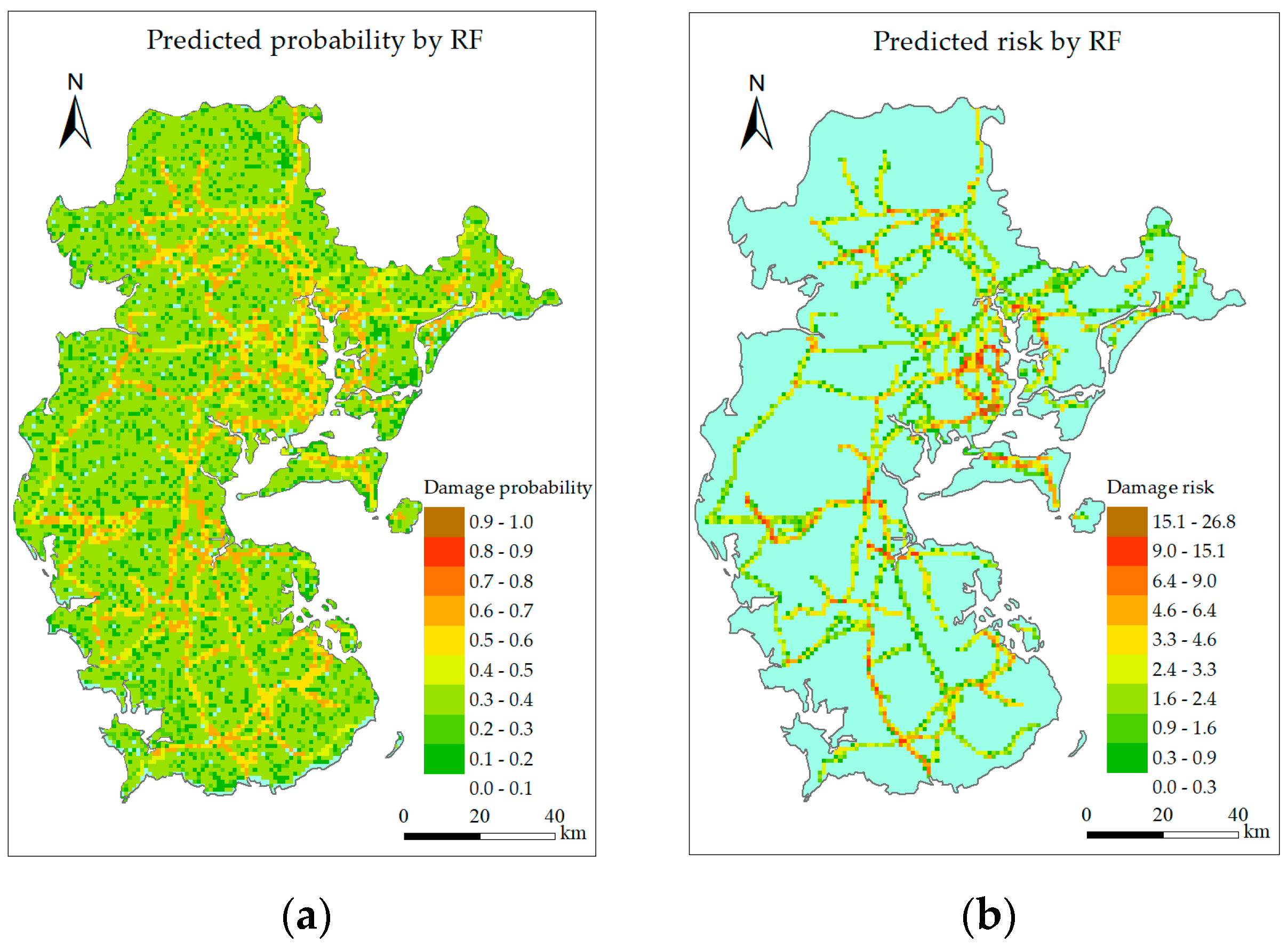
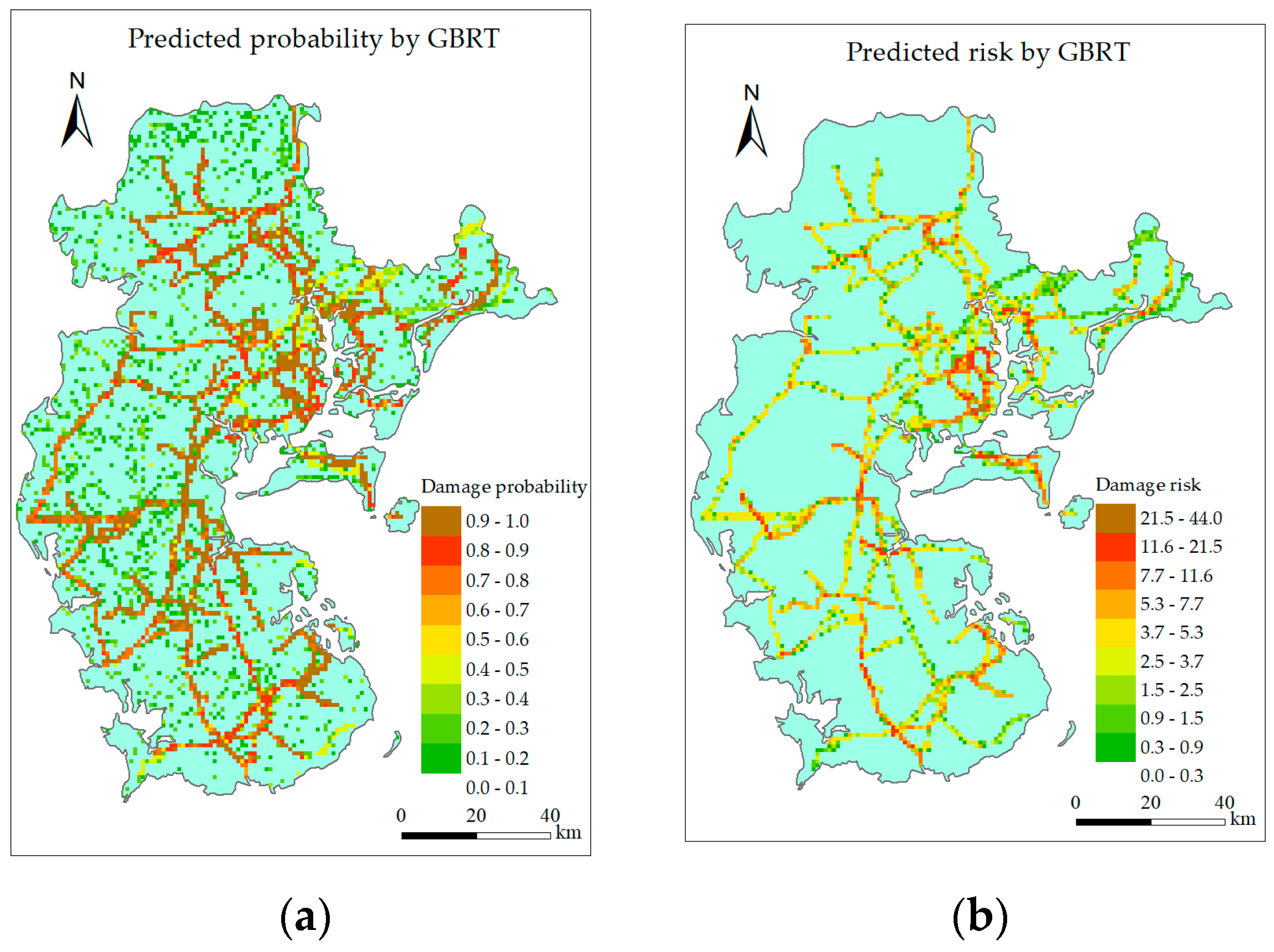
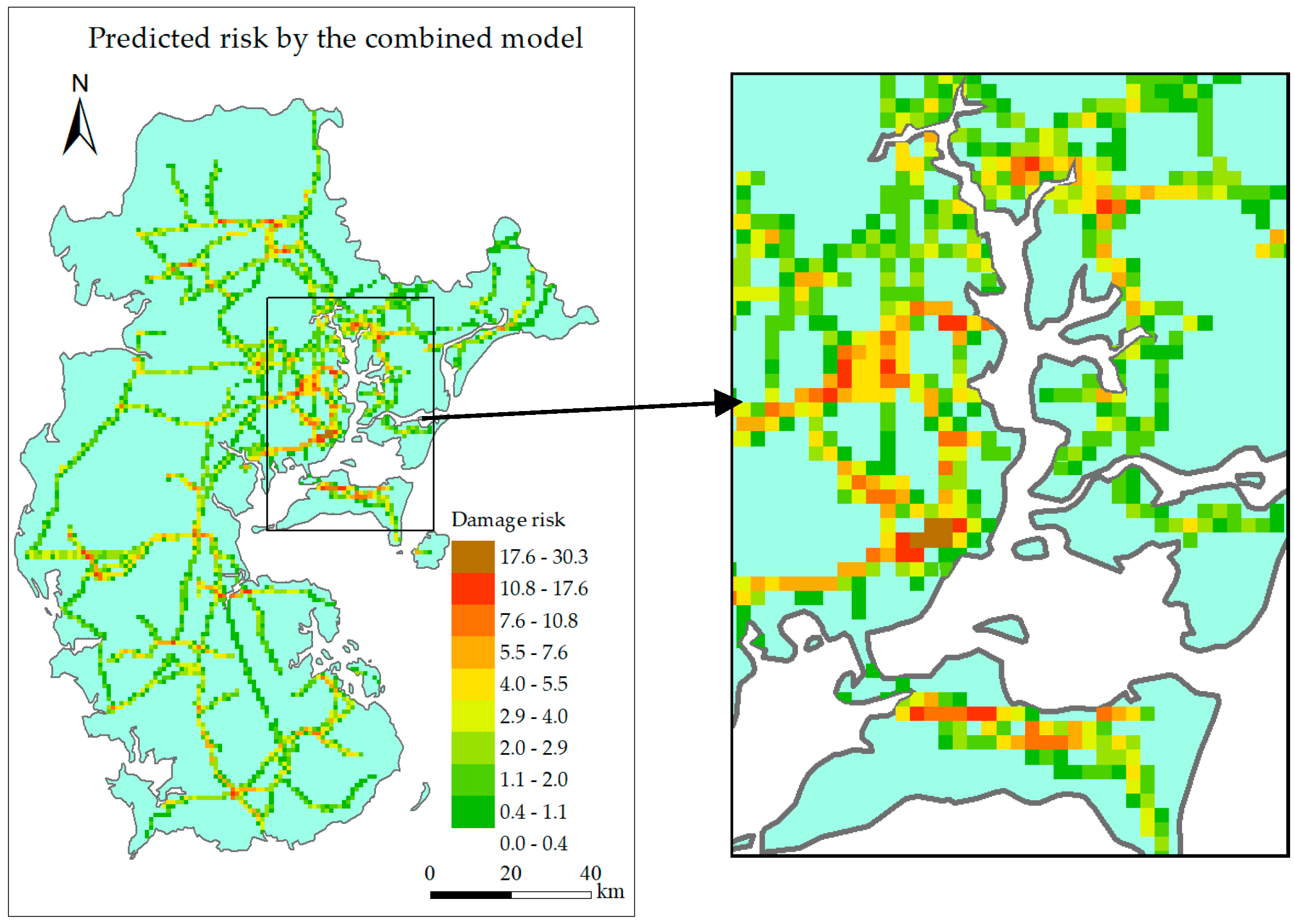
- RF, GBRT, and the combined model perform better than other models, but predicted risk distribution of the combined model is the most similar to the actual situation.
- (4)
- The similarity indicator of predicted risk of the combined model is 0.210 829, which is the biggest among all the models, so the combined model is the optimal model.
- (5)
- This study verifies the feasibility and scientificity of the presented method and can provide support for the power sector in disaster prevention and mitigation.
- (6)
- The uncertainty existing in the model should be tackled in the future for higher predicting accuracy, and it is necessary to extend the evaluation object to other power equipment such as transmission lines and transformers, and further raise from the equipment level to the system level.
Author Contributions
Funding
Conflicts of Interest
Appendix A

| Model | Hyperparameters for Optimization | Range | Optimized Hyperparameters |
|---|---|---|---|
| RF | criterion; n_estimators. | mse, mae; 1–100. | mae; 69. |
| GBRT | learning_rate; loss; n_estimators. | 0.01–1.0; ls, lad, huber, quantile; 1–200. | 0.203 578; huber; 190. |
| CART | criterion; presort; splitter. | mse, mae, friedman_mse; 0/1; best, random. | mae; 1; best. |
| SVR | C; coef0; degree; epsilon; gamma; kernel; shrinking. | 0–5; 0–10; 0–10; 0–10; 0–10; linear, poly, rbf, sigmoid; 0/1. | 3.894 502; 7.335 600; 3; 0.076 037; 5.350 016; rbf; 0. |
| Adaboost | learning_rate; loss; n_estimators. | 0.01–1; linear, square, exponential; 1–100. | 0.176 719; linear; 58 |
| LR | C; penalty. | 0–10; l1,l2. | 3.765 847; l1. |
Appendix B
Appendix B.1. SVR
Appendix B.2. CART
Appendix B.3. Adaboost
Appendix B.4. GBRT
References
- Zhou, X.M.; Ge, S.Y.; Li, T.; Liu, H. Assessing and Boosting Resilience of Distribution System Under Extreme Weather. Chin. Soc. Electron. Eng. 2018, 38, 505–513. [Google Scholar] [CrossRef]
- Yin, C.X.; Tang, W.Q.; Wen, L.F.; Lan, J.J.; Lin, J.H.; Li, S.Y.; Li, N. A new method for reliability evaluation of distribution network considering the influence of typhoon. Power Syst. Prot. Control 2018, 46, 138–143. [Google Scholar] [CrossRef]
- Song, X.Z.; Wang, Z.; Xin, H.H.; Gan, D.F. Risk-based dynamic security assessment under typhoon weather for power transmission system. In Proceedings of the IEEE PES Asia-Pacific Power and Energy Engineering Conference (APPEEC), Kowloon, China, 8–11 December 2013. [Google Scholar]
- Gao, W.; Zhou, R.; Zhao, D. Heuristic failure prediction model of transmission line under natural disasters. IET Gener. Transm. Distrib. 2017, 11, 935–942. [Google Scholar] [CrossRef]
- Huang, Z.; Wang, F.; Tan, Y.H.; Dong, X.Z.; Wu, Z.R.; Chen, C. Operational risk assessment based on health and importance indexes for distribution network. Electron. Power Autom. Equip. 2016, 36, 136–141. [Google Scholar] [CrossRef]
- Yang, L. Operational Statistic Risk Assessment for Power Systems Under Extreme Weather Conditions. In Proceedings of the Advances in Power System Control, Operation & Management (APSCOM 2015), 10th International Conference, Hong Kong, China, 8–12 November 2015. [Google Scholar]
- Yang, Y.H.; Xin, Y.L.; Zhou, J.J.; Tang, W.H.; Li, B. Failure probability estimation of transmission lines during typhoon based on tropical cyclone wind model and component vulnerability model. In Proceedings of the 2017 IEEE PES Asia-Pacific Power and Energy Engineering Conference (APPEEC), Bangalore, India, 8–10 November 2017. [Google Scholar]
- Han, L. Construction and Application of Emergency Management System for Power Network Disaster Prevention and Mitigation, 1st ed.; National Defense Industry Press: Beijing, China, 2009. [Google Scholar]
- Knowing Icing Early: Hunan Power Grid Disaster Prevention and Mitigation Technology Is at the International Leading Level. Available online: http://hn.rednet.cn/c/2015/01/15/3577523.htm (accessed on 8 June 2018).
- Wu, C.P.; Lu, J.Z.; Liu, Y.; Yang, L. Technology of field fire prevention near transmission lines and its application in Hunan power grid. Hunan Electron. Power 2014, 34, 28–30. [Google Scholar]
- Wang, J.; Shi, H.Y.; Fang, J.L. Discussion on GIS-based monitoring and early warning system for meteorological disasters in power grids. Autom. Appl. 2017, 5, 92–93. [Google Scholar]
- Liu, H.B.; Rachel, A.D.; David, V.R.; Jery, S. Negative binomial regression of electric power outages in hurricanes. J. Infrastruct. Syst. 2005, 11, 258–267. [Google Scholar] [CrossRef]
- Liu, H.B.; Rachel, A.D.; Tatiyana, V.A. Spatial generalized linear mixed models of electric power outages due to hurricanes and ice storms. Reliab. Eng. Syst. Saf. 2008, 93, 897–912. [Google Scholar] [CrossRef]
- Mensah, A.F.; Duenas-Osorio, L. Efficient Resilience Assessment Framework for Electric Power Systems Affected by Hurricane Events. J. Struct. Eng. 2016, 142, C4015013. [Google Scholar] [CrossRef]
- Han, S.; Guikema, S.D.; Quiring, S.M.; Lee, K.; Rosowsky, D.; Davidson, R.A. Estimating the spatial distribution of power outages during hurricanes in the Gulf Coast region. Reliab. Eng. Syst. Saf. 2009, 94, 199–210. [Google Scholar] [CrossRef]
- Han, S.; Guikema, S.D.; Quiring, S.M. Improving the Predictive Accuracy of Hurricane Power Outage Forecasts Using Generalized Additive Models. Risk Anal. 2009, 29, 1443–1453. [Google Scholar] [CrossRef] [PubMed]
- Sun, J.B.; Xin, T.; Wang, Y.W. Experience of Guangdong Power Grid Resisting Super Typhoon “Rammasun” and Introspection. Guangdong Electron. Power 2014, 27, 80–83. [Google Scholar] [CrossRef]
- Lyu, H.; Chen, Y.L.; Tang, Y.; Wang, L.H.; He, F.S.; Xie, W.P. Reason Analysis on Disconnector Damage After Typhoon “Rainbow”. Guangdong Electron. Power 2015, 28, 138–143. [Google Scholar] [CrossRef]
- Zhang, Z.Q. Application of double-strength main material in the reinforcement project of power tower in Zhuhai under typhoon “Hato”. Mech. Electron. Inf. 2017, 51–53. [Google Scholar] [CrossRef]
- Summary Report on the Impact of Typhoon “Mujigae” on Transmission Lines; Electric Power Research Institute, Guangdong Power Grid Co., Ltd.: Guangdong, China, 2015.
- Technical Specifications for Windproof Design of Distribution Lines of China Southern Power Grid Corporation; Q/CSG 1201012-2016; China Southern Power Grid Co., Ltd.: Guangzhou, China, 2016.
- Qu, C.X.; Jiang, Y.; Wu, Y.P.; Zou, X.N.; Qiao, Y.L. Study on the development of a choropleth atlas on cancer mortality using the inverse distance weight interpolation in the 1990’s. Chin. J. Epidemiol. 2006, 27, 230–233. [Google Scholar]
- Li, X.; Cheng, G.D.; Lu, L. Comparison of spatial interpolation methods. Adv. Earth Sci. 2000, 15, 260–265. [Google Scholar]
- Li, H. Statistical Learning Method, 1st ed.; Tsinghua University Press: Beijing, China, 2012. [Google Scholar]
- Vapnik, V. Statistic Learning Theory, 1st ed.; New York Wiley: New York, NY, USA, 1998. [Google Scholar]
- Leo, B.; Jerom, H.F.; Richard, A.O.; Charles, J.S. Classification and Regression Trees, 1st ed.; Chapman & Hall: New York, NY, USA, 1984. [Google Scholar]
- Zhao, Z.Y. Python Machine Learning Algorithm, 1st ed.; Publishing House of Electronics Industry: Beijing, China, 2017. [Google Scholar]
- Freund, Y.; Schapire, R.E. A decision-theoretic generalization of on-line learning and an application to Boosting. J. Comput. Syst. Sci. 1997, 55, 119–139. [Google Scholar] [CrossRef]
- Freund, Y.; Schapire, R.E. Experiments with a new Boosting algorithm. In Proceedings of the 13th Conference on Machine Learning, Bari, Italy, 3–6 July 1996. [Google Scholar]
- Friedman, J.H. Greedy function approximation: A gradient boosting machine. Ann. Stat. 2001, 29, 1189–1232. [Google Scholar] [CrossRef]
- Breiman, L. Random forests. Mach. Learn. 2001, 45, 5–32. [Google Scholar] [CrossRef]
- Wang, L.D.; Li, Z.Y.; Wen, J.Y. Short-term load fast forecasting based on support vector regression. RELAY 2005, 33, 17–20, 49. [Google Scholar] [CrossRef]
- Zhou, Z.H. Machine Learning, 1st ed.; Tsinghua University Press: Beijing, China, 2016. [Google Scholar]
- Scikit-Learn. Available online: http://sci-kit-learn.org/stable/index.html (accessed on 18 June 2018).
- Li, W.Y. Risk Assessment of Power System (Models, Methods and Applications), 1st ed.; Science Press: Beijing, China, 2006. [Google Scholar]
- Wei, Z.J.; Ma, H.L.; Tang, D.L. Trend Assessment of Typhoon Disasters Based on the Improved Entropy Method. J. Catastrophol. 2017, 32, 7–11. [Google Scholar] [CrossRef]


| Class | Surface Features | α |
|---|---|---|
| A | Offshore seas, islands, coasts, lakeshores, and desert areas | 0.10–0.13 |
| B | Fields, villages, jungles, hills, small and medium size towns, and suburbs of large cities where housing density is sparse | 0.13–0.18 |
| C | Urban areas with dense buildings | 0.18–0.28 |
| D | Urban area of a large city with dense buildings and tall houses | 0.28–0.44 |
| Feature Name | Meaning | Value Range |
|---|---|---|
| V10 (m/s) | Maximum gust at 10 m | 0–70 |
| V′10 (m/s) | Design wind at 10 m | 0–50 |
| H (m) | Altitude | −102–2483 |
| A (°) | Aspect | −1–360 |
| S (°) | Slope | 0–90 |
| P | Slope position | 0–3 |
| U | Underlying surface | 70–79 |
| R (m) | Surface roughness | 0–30 |
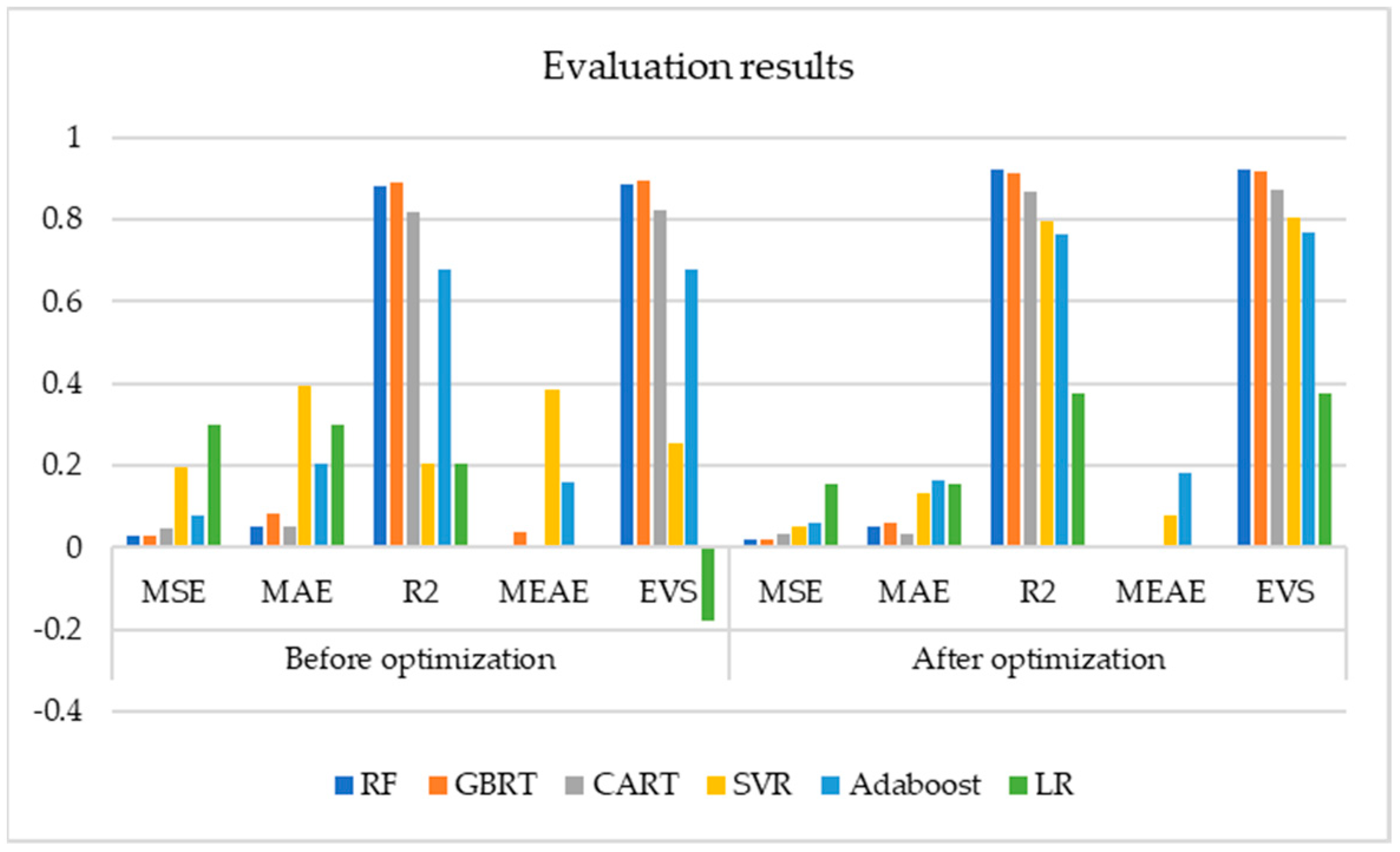
| Model | Before Optimization | After Optimization | ||||||||
|---|---|---|---|---|---|---|---|---|---|---|
| MSE | MAE | R2 | MEAE | ESV | MSE | MAE | R2 | MEAE | ESV | |
| RF | 0.0296 | 0.0529 | 0.880 | 0.000 | 0.886 | 0.0196 | 0.0503 | 0.920 | 0.007 | 0.922 |
| GBRT | 0.0267 | 0.0843 | 0.892 | 0.035 | 0.896 | 0.0213 | 0.058 | 0.914 | 0.003 | 0.916 |
| CART | 0.0451 | 0.0527 | 0.817 | 0.000 | 0.822 | 0.033 | 0.033 | 0.866 | 0.000 | 0.871 |
| SVR | 0.196 | 0.395 | 0.206 | 0.386 | 0.256 | 0.0502 | 0.131 | 0.796 | 0.076 | 0.803 |
| Adaboost | 0.0794 | 0.206 | 0.678 | 0.160 | 0.677 | 0.0577 | 0.165 | 0.766 | 0.182 | 0.769 |
| LR | 0.297 | 0.297 | 0.204 | 0.000 | −0.180 | 0.154 | 0.154 | 0.375 | 0.000 | 0.375 |
| Model | RF | GBRT | CART | SVR | Adaboost |
|---|---|---|---|---|---|
| weight | 0.212 441 | 0.210 846 | 0.201 265 | 0.189 891 | 0.185 557 |
| Model | RF | GBRT | CART | SVR | Adaboost | LR | Combined Model |
|---|---|---|---|---|---|---|---|
| S | 0.202 999 | 0.197 771 | 0.190 429 | 0.125 620 | 0.202 631 | 0.203 927 | 0.210 829 |
© 2019 by the authors. Licensee MDPI, Basel, Switzerland. This article is an open access article distributed under the terms and conditions of the Creative Commons Attribution (CC BY) license (http://creativecommons.org/licenses/by/4.0/).
Share and Cite
Hou, H.; Yu, S.; Wang, H.; Huang, Y.; Wu, H.; Xu, Y.; Li, X.; Geng, H. Risk Assessment and Its Visualization of Power Tower under Typhoon Disaster Based on Machine Learning Algorithms. Energies 2019, 12, 205. https://doi.org/10.3390/en12020205
Hou H, Yu S, Wang H, Huang Y, Wu H, Xu Y, Li X, Geng H. Risk Assessment and Its Visualization of Power Tower under Typhoon Disaster Based on Machine Learning Algorithms. Energies. 2019; 12(2):205. https://doi.org/10.3390/en12020205
Chicago/Turabian StyleHou, Hui, Shiwen Yu, Hongbin Wang, Yong Huang, Hao Wu, Yan Xu, Xianqiang Li, and Hao Geng. 2019. "Risk Assessment and Its Visualization of Power Tower under Typhoon Disaster Based on Machine Learning Algorithms" Energies 12, no. 2: 205. https://doi.org/10.3390/en12020205
APA StyleHou, H., Yu, S., Wang, H., Huang, Y., Wu, H., Xu, Y., Li, X., & Geng, H. (2019). Risk Assessment and Its Visualization of Power Tower under Typhoon Disaster Based on Machine Learning Algorithms. Energies, 12(2), 205. https://doi.org/10.3390/en12020205