Abstract
Sensorless brushless DC (BLDC) motor drive systems often suffer from inaccurate commutation signals, which result in current fluctuation and high conduction loss. To improve precision of commutation signals, this paper presents a novel commutation error compensation strategy for BLDC motors. First, the relationship between the line voltage difference integral in 60 electrical degree conduction interval and the commutation error is analyzed. Then, in terms of the relationship derived, a feedback compensation strategy based on the line voltage difference integral is proposed to regulate commutation signals by making three-phase back electromotive force (EMF) integral to zero, and the effect of the freewheeling process on the line voltage difference integral is considered. Moreover, an incremental PI controller is designed to achieve closed-loop compensation for the commutation error automatically. Finally, experiment results verify feasibility and effectiveness of the proposed strategy.
1. Introduction
Brushless DC (BLDC) motors are widely used in aerospace, electric vehicle, and household applications due to their inherent advantages, which include high-power density, high efficiency, and simple structure [1,2,3]. Position sensors, such as Hall-effect sensors, are often employed to acquire rotor position signals for proper commutation, however, misalignment in the mechanical installation of the sensors, extreme temperature conditions, or electromagnetic interference may induce errors in the rotor position information, which severely limit the application scope of BLDC motors [4]. To overcome these disadvantages, many sensorless BLDC motor techniques have been proposed in recent years. The zero-crossing points (ZCPs) of the back electromotive force (EMF) are easily detected and widely used in sensorless control. Among the various sensorless strategies currently available, these presented ZCP detection techniques show satisfactory results in specific application scopes; unfortunately, these strategies are still disturbed by various commutation errors [5,6,7]. The ZCPs of back-EMF are generally abstracted from the terminal voltage, but the terminal voltage is vulnerable to the high-frequency components due to the pulse-width modulation (PWM) switching. A low pass filter is usually applied to filter high-frequency switching noise of the terminal voltage, whereas the filters will introduce phase delay for ZCPs detection of back-EMF and the phase delay varies with the operating speed. The lag angle will increase as the motor speed rises. The distorted terminal voltage caused by the freewheeling process also will generate the commutation error. The disturbed terminal voltage may make position detection signal phase ahead, deviating from the ideal commutation instants. The inaccurate commutation signals will induce current pulsation and increase conduction loss.
In reference [8], a hysteresis comparator composed of discrete components is presented to compensate phase delay from the low-pass filter. In reference [9], the authors analyze the errors caused by signal extraction circuits and machine parameters in the sensorless control technique based on average line to line voltage. In reference [10], commutation errors due to the armature reaction and low-pass filters are analyzed, and an error compensation circuit is proposed to achieve proper commutation. In reference [11], the effects of the low-pass filter, noise, and nonideal properties of the estimated back-EMF on the commutation instants are considered. To adjust commutation instants for BLDC motors, a modified digital phase shifter is designed to implement compensation of commutation errors. In the research mentioned previously [8,9,10,11], some specific error factors are discussed and investigated, and the accuracy of the commutation signal is improved accordingly. To achieve more precise commutation signals of sensorless BLDC motors, the commutation error compensation strategies which consider more comprehensive error factors should be studied.
Many estimation and observer methods of commutation error compensation have been proposed to achieve high-precision commutation [12,13,14,15,16,17,18]. In reference [12], the torque constant is employed as the reference signal of the rotor position to obtain accurate commutation signals. In reference [13], the rotor position is acquired from the back-EMF difference, which is estimated from the disturbance observer structure. Discrete-time sliding mode observer [14] and iterative sliding mode observer [15] have been introduced to obtain precise commutation signals for sensorless permanent magnet synchronous motor control. Estimation strategies based on Kalman filters [16] and extended Kalman filters [17,18] have also been presented to estimate information of rotor position accurately. However, these algorithms are complicated and require a large amount of calculation.
Commutation error factors are reflected in the commutation signals, and thus voltages or currents under inaccurate commutation will contain the commutation error information. Many compensation strategies of commutation errors based on the phenomenon of voltages or currents produced under inaccurate commutation have been proposed. In reference [19], an intelligent self-tuning strategy is presented to finely adjust commutation instants, and regulation of the commutation instants is realized by minimizing the stator current. In reference [20], a self-compensation strategy of the commutation angle based on the DC-link current is proposed; in this technique, the commutation instants are corrected by regulating the estimated commutation time error to zero. However, this method is based on the linearized approximation between the DC-link current difference and commutation time error in low-inductance motors. In reference [21], commutation errors are compensated by keeping the freewheeling current of the unenergized phase symmetrical. However, when dealing with some PWM strategies featuring suppression of the freewheeling current [22], such as PWM_ON_PWM mode, the method is unsuitable. The research in [23] proposed a current index optimal approach to adjust commutation errors. However, the back-EMF is assumed to be a trapezoidal waveform with less than 120° flat-top width, which limits the applications of the proposed method. In reference [24], the symmetrical characteristics of the unenergized phase terminal voltage are presented to regulate commutation instants, but the effect of the freewheeling period is not considered.
This paper presents a novel compensation strategy for commutation errors of sensorless BLDC motors. In this paper, the relationship between the commutation error and the line voltage difference integral in 60 electrical degrees interval is analyzed, and a feedback compensation strategy based on the line voltage difference integral is presented to regulate commutation instants and the effect of the freewheeling period is considered. In addition, a PI controller is designed to achieve closed-loop compensation for commutation errors. The remainder of the paper is organized as follows. The proposed commutation error compensation strategy is proposed in Section 2. Section 3 provides experimental results to support the validity and effectiveness of the proposed method. The conclusions are presented in Section 4.
2. Proposed Commutation Error Compensation Strategy
This paper presents a commutation error compensation strategy based on the line voltage difference integral. In this section, the relationship between the line voltage difference integral and the commutation error is theoretically analyzed. Then, a feedback compensation strategy with the line voltage difference integral is presented. Finally, an incremental PI controller is designed to regulate the commutation error.
2.1. Mathematical Model of BLDC Motor
The equivalent circuit of the BLDC motor drive system is shown in Figure 1. Assuming that the three-phase stator windings are symmetrical, the phase resistance and inductance are constant, and the armature reaction is negligible. Then, the voltage equations are described as
where , , and are the three-phase voltages; , , and are the three-phase currents; , , and are the phase back-EMFs; is the stator resistance; is the phase inductance; and is the neutral voltage.
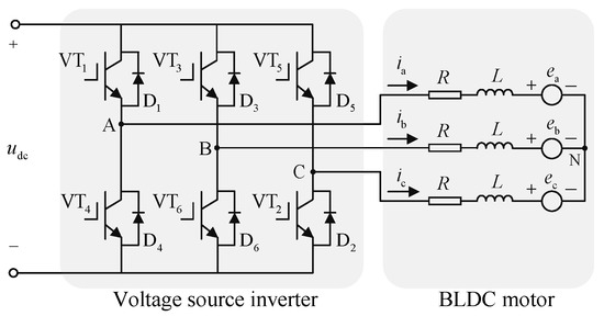
Figure 1.
Equivalent circuit of a brushless DC (BLDC) motor drive system.
The line voltage equations are expressed as
In general, the back-EMF of BLDC motors is between those of a trapezoidal wave and a sine wave since it contains many high-order harmonics. Hence, the back-EMF of the BLDC motor can be expressed as
where is the back-EMF coefficient; (2n + 1) is the order of harmonics; is the rotor position; , , and represent the mth harmonics of the three-phase back-EMF and the subscript m denotes harmonic order; and represent the third harmonics of the back-EMF.
Figure 2 shows phase diagram between back-EMFs and phase current, where , , and denote the back-EMFs, and , , and denote phase current. represents the commutation error, which is assumed . The sign of the commutation error reflects the commutation information (i.e., delayed or advanced commutation). A negative commutation error denotes advanced commutation, whereas a positive error represents a delayed one.
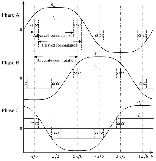
Figure 2.
Phase diagram of the back electromotive forces (EMFs) and phase current.
2.2. Line Voltage Difference Integral without Consideration of Freewheeling Period
For a BLDC motor, there are six operation modes and every operation modes last 60 electrical degrees. In the 60 electrical degree conduction interval, two periods are included: the freewheeling period and the normal conduction period. In the freewheeling period , the incoming phase current begins to rise, the un-commutated current remains conducting, and the outgoing phase current gradually decays due to the existence of phase inductance. When the outgoing phase current drops to zero, the freewheeling period is over and the motor starts operating in the normal conduction period.
Assume at some step that VT1 and VT6 are conducting, while VT5 is floating. The line voltage difference is expressed as
Considering a BLDC motor with a negligible freewheeling period , the current equation satisfies and during the entire 60-electrical degree period when , as shown in Figure 2. Substituting the current equation into (4), the line voltage difference is simplified as
By integrating (5), the line voltage difference integral is achieved as follows:
Figure 3 shows the three-phase back-EMF under accurate, delayed, and advanced commutation; the shadowed areas in each subfigure represent the integral of each back-EMF. As seen in Figure 3a, the integral of the back-EMFs and yields equal amplitudes but opposite signs, i.e., ; hence, the sum of the integrated back-EMFs and is zero in the interval. Similarly, the integral of the back-EMF is zero, i.e., , due to the AC symmetry of the back-EMF . From this analysis, (6) satisfies the condition
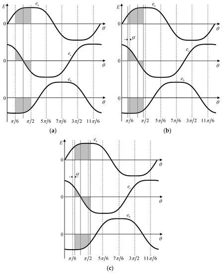
Figure 3.
Three-phase back-EMF. (a) Accurate commutation; (b) Advanced commutation; (c) Delayed commutation.
The line voltage difference integral under accurate commutation yields a value of zero. When the commutation instants are delayed or advanced by , the conduction period of VT1 and VT6 lasts for the interval , and the line voltage difference integral is written as
where , .
Since the third harmonics of the three three-phase back-EMFs are equal, . Then, (8) is simplified as
Solving and simplifying the definite integral gives
As the back-EMF harmonic coefficients satisfy the condition , the high-order terms of the back-EMF in (10) are negligible, and (10) can be simplified as
As seen in (11), the three-phase back-EMF integral is a function of the commutation error . The relationship between the three-phase back-EMF integral and the commutation error will be discussed in the following section.
Accurate commutation: when the commutation error , the motor works under accurate commutation, as shown in Figure 3a, and the back-EMF integral .
Advanced commutation: when the commutation error , the motor works under advanced commutation, as shown in Figure 3b, and the three-phase back-EMF integral .
Delayed commutation: when the commutation error , the motor works under delayed commutation, as shown in Figure 3c, and the three-phase back-EMF integral .
Similarly, when VT3 and VT4 are in conduction state, the phase current flows in opposite direction compared with the direction during the conduction period of VT1 and VT6. The three-phase back-EMF integral under accurate commutation, under delayed commutation, and under advanced commutation.
From previous research on three-phase back-EMF integral and the line voltage difference integral expression in (7), when the freewheeling period is negligible, the line voltage difference integral is proportional to the commutation error and can be used as an indicator of commutation errors.
The relationship between the conduction switch, the line voltage difference integral, and the commutation information is shown in Table 1; here, and are the lower and upper limits of integral, respectively.

Table 1.
Relationship between the integral , conduction switch, and commutation error.
When the motor is in no-load state, the effect of the freewheeling period is negligible. Figure 4 shows the diagram of the line voltage difference integral in the 60-electrical degree interval of A+B− and A−B+, where and represents the conduction period of phase A+B− and A−B+, respectively. The integral in the A+B− conduction interval is zero under accurate commutation (Figure 4a), negative under advanced commutation (Figure 4b), and positive under delayed commutation (Figure 4c). In the A−B+ conduction interval, the integral is opposite compared with that in the A+B− conduction interval. These results agree with the theoretical analysis.
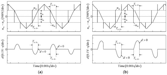
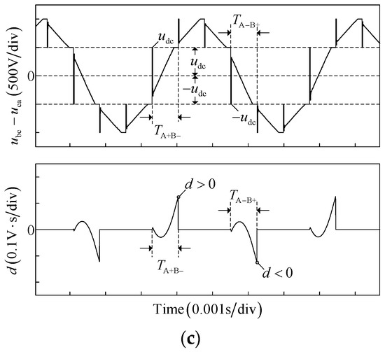
Figure 4.
Line voltage difference and integral in the conduction period of phase A+B− and A−B+. (a) Accurate commutation; (b) Advanced commutation; (c) Delayed commutation.
2.3. Line Voltage Difference Integral Considering Freewheeling Period
During the freewheeling period , the line voltage difference is distorted by the DC-link voltage and clamped at the level of the DC-link voltage . When line voltage difference integral is performed, the distorted line voltage difference in the interval is also integrated, which will cause the line voltage difference integral to deviate from the accurate line voltage difference integral. In this section, the line voltage difference integral of a BLDC motor considering the freewheeling period will be discussed.
Assume that the commutation error is and the conduction interval of VT1 and VT6 lasts for the period when , as shown in Figure 2. In the conduction period, the line voltage difference integral can be expressed as
Figure 5 shows the equivalent circuit when the commutation occurs from VT5 to VT1. In the commutation period , VT5 is turned off, VT1 is turned on, and VT6 continues conducting. The three phase voltages are expressed as
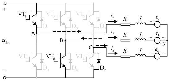
Figure 5.
Equivalent circuit when commutation occurs from VT5 to VT1.
The line voltage difference meets the condition , and the line voltage difference integral during the freewheeling period is reformulated as
In (14), the line voltage difference is equal to the DC-link voltage in the freewheeling period ; hence, the line voltage difference integral shows a trend of linear growth in the freewheeling period .
Figure 6 shows the diagram of the line voltage difference and its integral in the conduction period of phase A+B− and A−B+. The as seen in Figure 6, the line voltage difference is equal to the DC-link voltage in the freewheeling period and the corresponding integral linearly increases in the interval. Compared with that in Figure 4, since the disturbed voltage difference is integrated in the freewheeling period , the integral under different commutation produces an amplitude deviation. Especially under accurate commutation, for example, the integral deviates from zero, and becomes positive and negative in the conduction period of phase A+B− and A−B+, respectively.
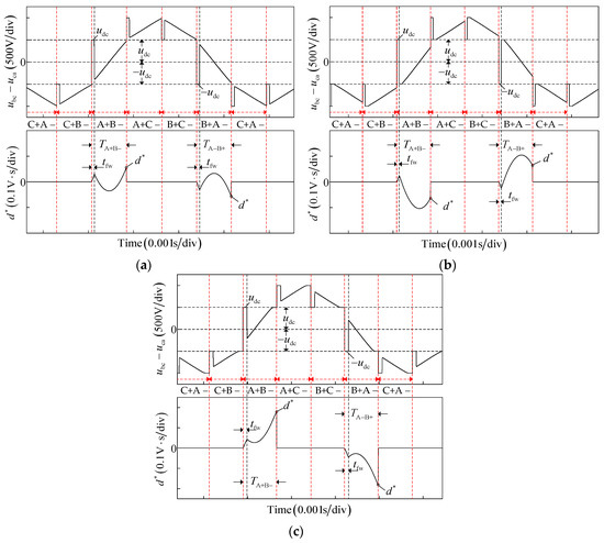
Figure 6.
The line voltage difference and corresponding integral in the conduction period of phase A+B− and A−B+. (a) Accurate commutation; (b) Advanced commutation; (c) Delayed commutation.
The other voltage spikes in Figure 6 are analyzed as followed. When the commutation occurs, the outgoing phase current continues conducting through the anti-parallel diode, so the terminal voltage is clamped at the level of 0 V or . When the motor commutates between different phases, the clamped voltage value of three-phase voltage changes, hence the line voltage difference will also change accordingly. The cause of the voltage spikes is the same under delayed, advanced, and accurate commutation. To facilitate the analysis, the voltage spike under the accurate commutation is taken as an example.
(1) When commutation occurs from A+B− to A+C−, it meets , , and in the freewheeling period . Therefore, , and it corresponds to the positive spike whose magnitude exceeds .
(2) When commutation occurs from B+A− to C+A−, it meets , , and in the freewheeling period . Therefore, , and it corresponds to the negative spike whose magnitude exceeds .
(3) When commutation occurs from A+C− to B+C−, it meets , , and in the freewheeling period . Therefore, , and it corresponds to the positive spike whose magnitude is equal to .
(4) When commutation occurs from C+A− to C+B−, it meets , , and in the freewheeling period . Therefore, , and it corresponds to the negative spike whose magnitude is equal to .
The voltage spikes of the line voltage difference in 360-degree electrical angle are listed in Table 2.
Table 2.
Voltage spike values in 360-degree electrical angle.
In the normal conduction period, when , the phase currents ia and ib conduct, while the outgoing phase current remains zero, i.e., and . Substituting the current equation and (2) into the second item of (12), the line voltage difference integral is rewritten as
By decomposing (15) into a combination of two items, it is reformulated as
Substituting (14) and (16) into (12), and (12) is rewritten as
The phase current satisfies in the freewheeling period . Substituting the phase current relationship, (13) into the second item of (17), it is simplified as
where is the final value of the outgoing phase current before commutation.
During the commutation period , the outgoing phase current drops from the final value to zero, the integral item can be approximated by , and (18) is rewritten as
From (13), the phase current in the freewheeling period is solved as
where .
From (20), the freewheeling period for the outgoing phase current dropping from final value to zero is solved as
Substituting (21) into (19), and (19) is shown as
In (22), is related to . Next, the effect of will be discussed.
In the freewheeling period when , is expressed as
Considering , the high-order terms of the back-EMF in (23) are negligible, and (23) can be simplified as
By calculating the trigonometric functions, (24) is simplified as
Both sides of (25) are multiplied by , and refined as
In general, the EMF harmonic coefficients of a BLDC motor with a trapezoidal back EMF [25] . The relationship between , , and the commutation error during the freewheeling period can be obtained in (26). When , , and the corresponding 3-D graph is shown in Figure 7a. It is observed that with respect to , is greater than zero when the commutation error , so . When , , and the corresponding 3-D graph is shown in Figure 7b. is less than zero when the commutation error , and . Based on the relationship, it is derived that and . Both sides of are multiplied by , and the item is represented as , where denotes copper loss and . denotes the input power of the motor and . In general, the copper loss is negligible, hence it satisfies , which implies Therefore, (19) is simplified as
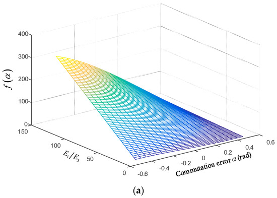
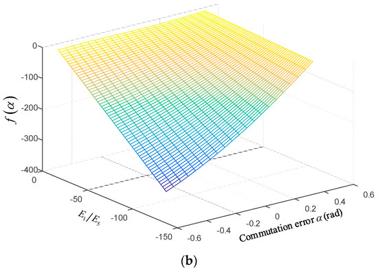
Figure 7.
Relationships between , , and the commutation error during the freewheeling period . (a) ; (b) .
Combining (27) and (17), the latter is reformulated as
According to the previous analysis, the general function of the line voltage difference integral is given as
where the subscripts x and y represent the active phase, and z represents the inactive phase. and are the lower and upper limits of integral, respectively.
2.4. Commutation Error Compensation Strategy
In Section 2.2 and Section 2.3, the respective line voltage difference integrals and without and with consideration of the freewheeling period are discussed. Next, the commutation error compensation strategy is described based on the analysis of the line voltage difference integral.
From (29), the three-phase back-EMF integral is rewritten as
According to the research in Section 2.2, three-phase back-EMF integral can reflect commutation errors. In (30), three-phase back-EMF integral can be obtained from the combination of the integral and to determine commutation errors when the freewheeling period is considered.
In general, the commutation instants are obtained by delaying ZCPs by 30 electrical degrees in the sensorless technique and reactivating the motor windings according to the predefined commutation sequence. The predefined commutation sequences are shown in Table 3; here, , , and are virtual hall signals.
Table 3.
Predefined commutation sequence.
In Table 1, the sign of the three-phase back-EMF integral changes according to the direction of the phase current. The three-phase back-EMF integral can be updated as
where denotes the rotation direction of the motor rotor. When , the motor runs in the anti-clockwise rotation, and when , the motor rotates in the opposite one. When the sensorless BLDC motor runs, the windings are excited in according with the predefined commutation sequence listed in Table 3, and the conduction switches are obtained. Then the line voltage difference integral is calculated with Table 1, and the outgoing phase current before commutation is sampled. By using (30), the three-phase back-EMF integral can be given. Considering the rotation direction of the motor rotor is known, the three-phase back-EMF integral is converted to a positive value under delayed commutation and to a negative one under advanced commutation with (31), which also makes PI controller available.
Here, a PI regulator is also designed to compensate commutation errors, and the PI regulator is defined as
where three-phase back-EMF integral error , and the reference value . is the proportional coefficient, and is the integral coefficient. is the integral period and . is the kth output value of the PI regulator, is the th output value of the PI regulator. Here, k represents the number of iterations.
For the sensorless BLDC motor based on ZCP detection of the back-EMF, the accurate commutation instants are obtained by 30 electrical degrees delayed shift of ZCPs. Therefore, after the commutation error is determined, the commutation shift is updated as
where .
Figure 8 shows the block diagram of a sensorless BLDC motor drive system and the proposed commutation error compensation strategy is shown in the shadowed area. The system contains a speed-loop controller, a current-loop controller, and a commutation error compensation link. In the commutation error compensation link, when commutation signals are detected, the outgoing phase current final value is sampled and the line voltage difference is integrated until the commutation occurs again. Then, the line voltage difference integral is recorded, and the three-phase back-EMF integral is calculated from the sampled current value and the line voltage difference integral . The entire compensation process is then resumed. A flowchart of the proposed method is shown in Figure 9.
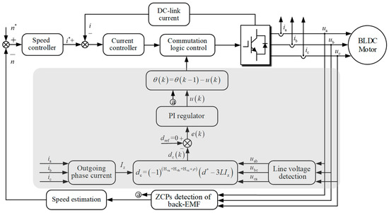
Figure 8.
Sensorless BLDC motor drive system with the proposed strategy.
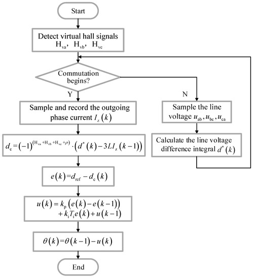
Figure 9.
Flowchart of the commutation error compensation procedure.
Figure 10 shows the back-EMF waveforms by the constant speed test of 1200 rpm.
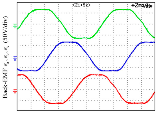
Figure 10.
Measured back-EMF waveforms of the BLDC motor at 1200 rpm.
3. Experiment Results
An experimental prototype is set up to verify the feasibility and effectiveness of the proposed strategy. The experimental platform, which consists of the control system and the experimental motor, is shown in Figure 11. The BLDC motor is connected to the generator by a flexible coupling, and its rated parameters are shown in Table 4. The core processor is DSP (TMS320F28335) with a 150 MHz clock frequency, and the three-phase inverter is IPM PM50RL1A060 (Mitsubishi). The line voltage and phase current are sampled by three voltage sensors (LV25-P) and three current sensors (LTS15-NP), respectively. To remove the effect of switching noise, a low-pass FIR filter with the Hamming window function was designed. The cutoff frequency and the order of the filter were selected as 3 kHz and 50, respectively. The filter provides 65 dB of signal attenuation at the switching frequency. Many experiments were conducted to obtain the proportional coefficient and the integral coefficient of the PI regulator. Based on the test results, the proportional coefficient and integral coefficient are designed as and , respectively. The modulation method of the three-phase inverter is PWM-ON, and the switching frequency of three-phase inverter and the sampling frequency of the line voltage are 10 and 200 kHz, respectively. The experimental results were monitored and recorded by a digital oscilloscope DL750 (YOKOGAWA), and the line voltage difference integral was observed through a DAC.
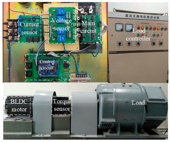
Figure 11.
Experimental setup of the BLDC motor drive system.
Table 4.
Motor parameters.
Figure 12 shows the phase current and the line voltage difference integral under advanced, delayed, and accurate commutation. In the experiment, the motor runs at a speed of 500 rpm, the load torque is 7.5 Nm, and the commutation instants are set to be advanced and delayed by 10°. The conduction periods of A+B− and A−B+ are taken as examples, and the outgoing phase current final value before commutation and the line voltage difference integral are marked in solid circles. In Figure 12a,b, there is an obvious current ripple in phase current and the line voltage difference integral is different. Figure 12c shows that the current ripple is attenuated obviously and the integral also changes correspondingly when the commutation instants are accurate. In addition, as shown in the dashed circle, the line voltage difference integral takes on an approximately linear variation trend during the freewheeling period .The experimental results are consistent with the theoretical analysis.
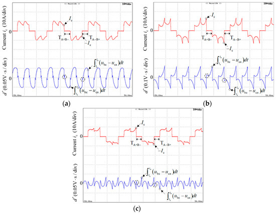
Figure 12.
Phase current and the line voltage difference integral. (a) Advanced commutation; (b) Delayed commutation; (c) Exact commutation.
The performance of the proposed strategy is tested in the steady and transient states. In the steady-state experiment, the motor runs at a fixed speed and load. In the transient experiment, the motor works at varying speeds and a fixed load. Figure 13 shows the phase currents and integral before and after compensation under different test conditions. It is observed that the phase current and the integral fluctuates obviously under delayed and advanced commutation, yet the current ripple is effectively reduced after the proposed compensation strategy is used, and the integral also changes correspondingly when the commutation instants are accurate. The experimental results show that the proposed strategy can accurately compensate commutation errors at different speeds and load torques.
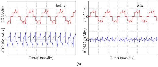
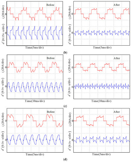
Figure 13.
Current waveform of phase C before and after compensation. (a) Commutation instants are delayed by 10° at a speed of 1000 rpm and load torque of 12 Nm; (b) Commutation instants are delayed by 12° at a speed of 1500 rpm and load torque of 16 Nm; (c) Commutation instants are advanced by 12° at a speed of 850 rpm and load torque of 10 Nm; (d) Commutation instants are advanced by 14° at a speed of 1200 rpm and load torque of 14 Nm.
Subsequently, the performance of the proposed strategy during the transient process is tested. In the experiment, the commutation instants are delayed by about 10°, and the motor is accelerated from 300 rpm to 1500 rpm at a load torque of 12 Nm. Figure 14 shows the phase current, the line voltage difference integral, and their enlarged vision with the proposed strategy. When the motor speed ramps up, the compensation strategy is initiated at the points S1 and S2, and the commutation error is almost removed at the points T1 and T2, respectively. It is seen that, after the compensation strategy is activated, the current fluctuation is effectively reduced. Therefore, the proposed compensation strategy exhibits satisfactory dynamic performance during variable-speed operation.
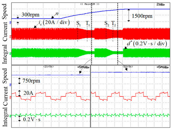
Figure 14.
Transient performance and enlarged view with the proposed strategy when the motor accelerates from 300 to 1500 rpm.
To test the convergence rate of the proposed strategy under the steady speed operation, the commutation error is set to about 10°, and the motor runs at a speed of 800 rpm and load torque of 12 Nm. Figure 15 shows the phase current, the line voltage difference integral , and their enlarged vision with PI controller. It is found that, before the point of Sa, the phase current curls up and the integral is high, while the compensation strategy with PI controller is activated at the point Sa, the current ripple and the integral gradually decreases. After 1.05 s, the current fluctuation is effectively suppressed, and the commutation error is almost eliminated. In addition, the convergence rate of the proposed method is tested at different speeds, and the test results are shown in Table 5, and the results show the proposed strategy converges quickly in a wide speed range.
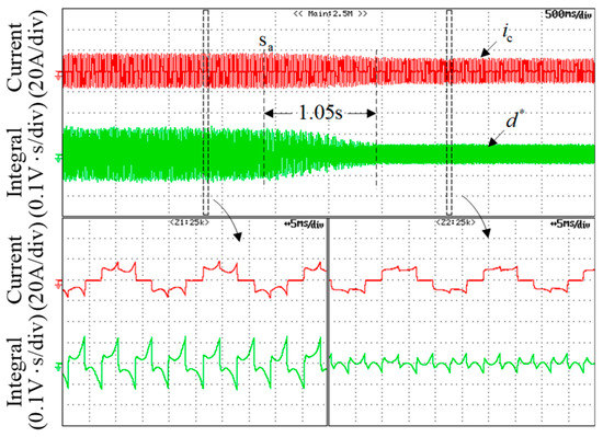
Figure 15.
Comparative results of the phase current, the integral of the line voltage difference, and their enlarged view at a speed of 800 rpm and load torque of 12 Nm.
Table 5.
Convergence rate of proposed strategy.
Moreover, the power consumption is reduced after the commutation instants are compensated with the proposed strategy. In these power consumption tests, the commutation instants are set to be delayed and advanced by 10°and 12°, respectively, the speed range is 300–1500 rpm and the load torques are about 11, 12, 13 and 15 Nm. Figure 16 shows the power consumption of the BLDC motor before and after compensation after steady operation for 40 min. The experimental results in Figure 16 show that the proposed strategy can reduce power consumption over wide speed ranges, especially in the high-speed ranges.
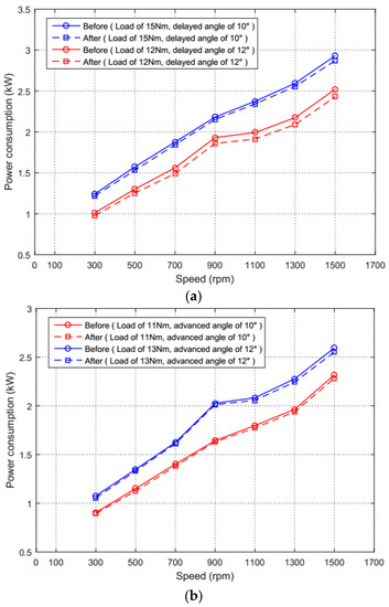
Figure 16.
Power consumption comparison before and after compensation. (a) Under delayed commutation; (b) Under advanced commutation.
4. Conclusions
This paper presents a novel compensation strategy for commutation error of sensorless BLDC motors. The method is suitable in both the steady-speed and variable-speed range. The relationship between the line voltage difference integral in 60 electrical degrees interval and the commutation error is established. A commutation error commutation strategy with respect of the line voltage difference integral is proposed to correct the inaccurate commutation instants by regulating the three-phase back-EMF integral to zero. In this method, the influence of the voltage pulses caused by the diode-freewheeling conduction on the line voltage difference integral is analyzed, making the proposed strategy applicable to BLDC motors considering the freewheeling period. Furthermore, a PI controller is also designed to realize closed-loop compensation for commutation errors. Finally, experimental results show the effectiveness and feasibility of the proposed strategy under different test conditions.
Author Contributions
This paper is the result of the hard work of all of the authors. X.Y. and J.Z. conceived and designed the proposed method. X.Y. and J.Z. conceived and analyzed the data. X.Y. provided funding support. J.Z. and G.L. conducted the experiment and verified the proposed method. J.Z., G.L., and H.L. wrote the paper, and H.L. and J.W. contributed to the review of the document. All authors gave advice for the manuscript.
Funding
This work was supported by the High-tech Ship Project of China under Grant No. GJYF-043/6.
Conflicts of Interest
The authors declare no conflict of interest.
References
- Capolino, G.A.; Cavagnino, A. New trends in electrical machines technology—Part I. IEEE Trans. Ind. Electron. 2014, 61, 4281–4285. [Google Scholar] [CrossRef]
- Acarnley, P.P.; Watson, J.F. Review of position-sensorless operation of brushless permanent-magnet machines. IEEE Trans. Ind. Electron. 2006, 53, 352–362. [Google Scholar] [CrossRef]
- Samoylenko, N.; Han, Q.; Jatskevich, J. Dynamic performance of brushless DC motors with unbalanced hall sensors. IEEE Trans. Energy Convers. 2008, 23, 752–763. [Google Scholar] [CrossRef]
- Hwang, C.; Li, P.; Chuang, F.; Liu, C.; Huang, K. Optimization for reduction of torque ripple in an axial flux permanent magnet machine. IEEE Trans. Magn. 2009, 45, 1760–1763. [Google Scholar] [CrossRef]
- Yang, Y.; Ting, Y. Improved angular displacement estimation based on Hall-effect sensors for driving a brushless permanent-magnet motor. IEEE Trans. Ind. Electron. 2014, 61, 504–511. [Google Scholar] [CrossRef]
- Cheng, C.; Cheng, M. Implementation of a highly reliable hybrid electric scooter drive. IEEE Trans. Ind. Electron. 2007, 54, 2462–2473. [Google Scholar] [CrossRef]
- Huang, X.; Goodman, A.; Gerada, C.; Fang, Y.; Lu, Q. A single sided matrix converter drive for a brushless DC motor in aerospace applications. IEEE Trans. Ind. Electron. 2012, 59, 3542–3552. [Google Scholar] [CrossRef]
- Chun, T.; Tran, Q.; Lee, H.; Kim, H. Sensorless control of BLDC motor drive for an automotive fuel pump using a hysteresis comparator. IEEE Trans. Power Electron. 2014, 29, 1382–1391. [Google Scholar] [CrossRef]
- Bhogineni, S.; Rajagopal, K.R. Position error in sensorless control of brushless dc motor based on average line to line voltages. In Proceedings of the IEEE International Conference on Power Electronics, Drives and Energy Systems (PEDES), Karnataka, India, 16–19 December 2012; pp. 1–6. [Google Scholar]
- Shen, J.; Tseng, K. Analyses and compensation of rotor position detection error in sensorless PM brushless DC motor drives. IEEE Trans. Energy Convers. 2003, 18, 87–93. [Google Scholar] [CrossRef]
- Cheng, K.; Tzou, Y. Design of a sensorless commutation IC for BLDC motors. IEEE Trans. Power Electron. 2003, 18, 1365–1375. [Google Scholar] [CrossRef]
- Park, J.; Hwang, S.; Kim, J. Sensorless control of brushless DC motors with torque constant estimation for home appliances. IEEE Trans. Ind. Appl. 2012, 48, 677–683. [Google Scholar] [CrossRef]
- Wang, S.; Lee, A. A 12-step sensorless drive for brushless DC motors based on back-EMF differences. IEEE Trans. Energy Convers. 2015, 30, 646–654. [Google Scholar] [CrossRef]
- Bernardes, T.; Montagner, V.F.; Grundling, H.A.; Pinheiro, H. Discrete-time sliding mode observer for sensorless vector control of permanent magnet synchronous machine. IEEE Trans. Ind. Electron. 2014, 61, 1679–1691. [Google Scholar] [CrossRef]
- Lee, H.; Lee, J. Design of iterative sliding mode observer for sensorless PMSM control. IEEE Trans. Control. Syst. Technol. 2013, 21, 1394–1399. [Google Scholar] [CrossRef]
- Alonge, F.; D’Ippolito, F.; Sferlazza, A. Sensorless control of induction-motor drive based on robust Kalman filter and adaptive speed estimation. IEEE Trans. Ind. Electron. 2014, 61, 1444–1453. [Google Scholar] [CrossRef]
- Quang, N.K.; Hieu, N.T.; Ha, Q.P. FPGA-based sensorless PMSM speed control using reduced-order extended kalman filters. IEEE Trans. Ind. Electron. 2014, 61, 4574–4582. [Google Scholar] [CrossRef]
- Idkhajine, L.; Monmasson, E.; Maalouf, A. Fully FPGA-based sensorless control for synchronous AC drive using an extended Kalman filter. IEEE Trans. Ind. Electron. 2012, 59, 3908–3918. [Google Scholar] [CrossRef]
- Chen, H.C.; Liaw, C.M. Sensorless control via intelligent commutation tuning for brushless dc motor. Inst. Electron. Eng. Electron. Power Appl. 2002, 46, 678–684. [Google Scholar] [CrossRef]
- Fang, J.; Li, W.; Li, H. Self-compensation of the commutation angle based on dc-link current for high-speed brushless DC motors with low inductance. IEEE Trans. Power Electron. 2014, 29, 428–439. [Google Scholar] [CrossRef]
- Wu, X.; Zhou, B.; Song, F.; Chen, F.; Wei, J. A closed loop control method to correct position phase for sensorless Brushless DC motor. In Proceedings of the International Conference on Electrical Machines and Systems, Wuhan, China, 17–20 October 2008; pp. 1460–1464. [Google Scholar]
- Krishnan, G.; Ajmal, K.T. A neoteric method based on PWM ON PWM scheme with buck converter for torque ripple minimization in BLDC drive. In Proceedings of the Annual International Conference on Emerging Research Areas: Magnetics, Machines and Drives (AICERA/iCMMD), Kottayam, India, 24–26 July 2014; pp. 1–6. [Google Scholar]
- Lee, A.; Wang, S.; Fan, C. A current index approach to compensate commutation phase error for sensorless brushless dc motor with non-ideal back EMF. IEEE Trans. Power Electron. 2016, 31, 4389–4399. [Google Scholar] [CrossRef]
- Jang, G.; Kim, M. Optimal commutation of a BLDC motor by utilizing the symmetric terminal voltage. IEEE Trans. Magn. 2006, 42, 3473–3475. [Google Scholar] [CrossRef]
- Zhou, X.; Chen, X.; Lu, M.; Zeng, F. Rapid self-compensation method of commutation phase error for low inductance BLDC motor. IEEE Trans. Ind. Inform. 2017, 13, 1833–1842. [Google Scholar] [CrossRef]
© 2019 by the authors. Licensee MDPI, Basel, Switzerland. This article is an open access article distributed under the terms and conditions of the Creative Commons Attribution (CC BY) license (http://creativecommons.org/licenses/by/4.0/).