Article

Optimal Preventive Maintenance of Wind Turbine Components with Imperfect Continuous Condition Monitoring

1
Projects and Maintenance Section, The Private Department of the President of the United Arab Emirates, Abu Dhabi 000372, UAE
2
Research and Development Department, Mathematical Modelling & Research Holding Limited, London W1W 7LT, UK
3
Department of Electronics, Robotics, Monitoring Technology, and IoT, National Aviation University, 03058 Kyiv, Ukraine
*
Author to whom correspondence should be addressed.
Energies 2019, 12(19), 3801; https://doi.org/10.3390/en12193801
Submission received: 17 June 2019 / Revised: 15 September 2019 / Accepted: 15 September 2019 / Published: 8 October 2019
(This article belongs to the Special Issue Maintenance Management of Wind Turbines)

Abstract

:
Among the different maintenance techniques applied to wind turbine (WT) components, online condition monitoring is probably the most promising technique. The maintenance models based on online condition monitoring have been examined in many studies. However, no study has considered preventive maintenance models with incorporated probabilities of correct and incorrect decisions made during continuous condition monitoring. This article presents a mathematical model of preventive maintenance, with imperfect continuous condition monitoring of the WT components. For the first time, the article introduces generalized expressions for calculating the interval probabilities of false positive, true positive, false negative, and true negative when continuously monitoring the condition of a WT component. Mathematical equations that allow for calculating the expected cost of maintenance per unit of time and the average lifetime maintenance cost are derived for an arbitrary distribution of time to degradation failure. A numerical example of WT blades maintenance illustrates that preventive maintenance with online condition monitoring reduces the average lifetime maintenance cost by 11.8 times, as compared to corrective maintenance, and by at least 4.2 and 2.6 times, compared with predetermined preventive maintenance for low and high crack initiation rates, respectively.

Graphical Abstract

1. Introduction

Currently, there is a global transformation of energy production toward renewable energy sources, and wind power is a source that is developing at the highest rate. According to the authors of [1], the overall capacity of all wind turbines (WTs) installed worldwide, by the end of 2018, was 597 GW, of which 50.1 GW was added in 2018 alone. Thus, the increase in wind power amounted to 8.4% in 2018. Wind power developed most rapidly in China and the United States, adding 21 GW and 7.6 GW in 2018, reaching 217 GW and 96 GW, respectively [1]. With such rapid growth of wind energy production, special attention is given to the lowered cost of 1 kWh of produced energy. Thus, according to IRENA [2], 1 kWh of energy produced by an offshore WT has decreased from 0.17 USD/kWh in 2010 to 0.14 USD/kWh in 2017. A significant reduction in the cost of produced wind energy can be achieved by reducing the cost of operation and maintenance (O&M). Indeed, O&M costs for offshore wind farms account for 25% of the total cost [3]. Therefore, many scientific publications have been devoted to optimizing the maintenance of WT [4,5,6,7,8,9,10].
When analyzing possible maintenance strategies for WT components, we use the terminology of the standard EN 13306: 2017 [11]. By this standard, the following basic maintenance types can be applied to WT components: preventive, predetermined, condition-based, corrective, and predictive.
Traditionally, preventive maintenance has relied on statistics data calculating such reliability indicators as mean time to failure, and the cumulative distribution function of time to failure to determine the optimum periodicity of component replacement. Preventive maintenance without previous condition investigation is called predetermined maintenance [11]. The main effect achieved when using predetermined preventive maintenance is reducing the probability of failure in the interval between services. Today, however, preventive maintenance activities can be effectively improved by using built-in sensors that can directly monitor the component condition. When using information from sensors, the operator observes an approaching failure, which allows for planning the necessary actions to replace the component and minimize potential losses.
Condition-based maintenance (CBM) is also preventive maintenance, but it includes a combination of condition monitoring and corresponding maintenance actions. Condition monitoring can be either scheduled or continuous. A distinctive feature of condition-based maintenance is the introduction of a preventive or replacement threshold, which is different from the degradation failure threshold.
Corrective maintenance is carried out after failure occurrence and intended to restore the component operability. Corrective maintenance is typically used for components which have failures that are not safety-related and do not lead to significant economic losses. Corrective maintenance may also use periodic inspections or continuous condition monitoring on the base of sensors; however, maintenance actions are performed only after failure identification.
Predictive maintenance comprises condition monitoring and forecasting the future component condition, where maintenance decision-making depends on the results of the prediction, so that the component can be replaced or restored before its failure. Predictive maintenance can also be based on periodic or continuous condition monitoring. However, the information obtained during monitoring is used to estimate the remaining useful life and to plan maintenance actions.
Thus, all of the types of maintenance considered, except for predetermined, are based on varying degrees of condition monitoring. The literature [12,13,14] gives a comprehensive analysis and discussion of condition monitoring methods used for WT components. The authors of [15] present an in-depth analysis of CBM strategies for offshore wind energy equipment. Currently, the most promising type of condition monitoring is the use of sensors that provide reliable continuous measurements and targeted evaluation of critical data. The use of sensors allows for avoiding manual inspections, reducing the probability of failure occurrence, reducing the downtime, and helping to plan maintenance actions [16]. Therefore, we will further highlight the studies on the optimization of the maintenance of deteriorating WT components using continuous condition monitoring.
Byon et al. [4] considered optimal repair strategies for WT that operate in different weather conditions. It is assumed that the sensors are error-free, and instantaneously reveal the system condition. Yildirim et al. [6] considered an integrated framework for wind farm maintenance that uses real-time sensor data to improve wind farm maintenance and operational decisions. A dynamic maintenance cost associated with preventive and corrective maintenance decisions is proposed. The study performed by Canizo et al. [17] presented a big data analytical approach for predictive maintenance of WT using a big data processing framework to generate predictive models based on historical data. Interactive fault-tolerant monitoring predicts the state of WT every 10 minutes. Fu et al. [18] considered a method for analyzing the reliability of a network monitoring wind turbine blades based on wireless sensor networks. Krishna [19] considered a remote instrument monitoring system, which is a dispatching control and data acquisition system based on a wireless sensor network, with a set of sensors distributed throughout the turbines of wind power plants. Nilsson and Bertling [20] presented a lifecycle cost analysis of different preventive and corrective maintenance strategies of WT, where a condition monitoring system is used to improve maintenance planning for a single WT onshore and a wind farm offshore. Kerres et al. [21] considered a model that is capable of estimating O&M cost for different maintenance strategies over the WT lifecycle. Three simulated types of maintenance include run-to-failure maintenance, maintenance with annual inspections of the gearbox and generator, as well as the installation of a vibration condition monitoring system that detects 90% of the gearbox and generator defects. Van Horenbeek et al. [22] considered a new concept of modeling various failure modes based on the P–F curve. The constructed stochastic simulation model allows for quantifying the economic benefits of introducing an imperfect condition monitoring system in the WT gearbox. Research proves that a condition monitoring system is beneficial, in comparison to the current maintenance strategy. Kaiser and Gebraeel [23] considered a sensory-updated predictive maintenance policy, which uses degradation models and sensor signals to predict and update the residual life distribution. Bryant and John [24] considered an asset management model of WT based on the method of modeling Petri nets. The condition monitoring system continuously monitors WT components to capture early indication of component failure, so that preventive maintenance can be planned. Besnard and Bertling [25] considered three maintenance strategies of WT blades, including visual inspections, inspection with a condition-monitoring technique, and online condition monitoring. The expected lifecycle maintenance costs associated with different approaches are calculated and compared. Pattison et al. [26] considered a new architecture for the implementation of reliability-centered maintenance of offshore WT. The architecture supposes three integrated modules for intelligent condition monitoring, reliability, and maintenance modeling, as well as maintenance schedules that provide cost-effective preventive maintenance management of offshore WTs. Ghamlouch et al. [27] considered a preventive maintenance model for a system subject to uncertainty due to the stochastic nature of the deterioration and production processes. Shafiee and Finkelstein [28] considered an optimal proactive maintenance policy for continuous monitoring systems prone to stochastic degradation. The task of proactive group maintenance is performed when the degradation level of the subsystem exceeds the “alert” threshold (less than the failure threshold), which reduces the probability of system failures. Shafiee et al. [29] considered an optimal CBM strategy for a multi-blade offshore wind turbine system subjected to stress corrosion cracking and environmental shocks. Wang et al. [30] considered a new model for diagnosing faults and predicting the remaining useful life of WT components with limited degradation data. The model can be used for predictive maintenance optimization of WT components. Marugan et al. [31] considered a novel approach for false alarm detection and prioritization applied to a real dataset from a vibration monitoring system of a WT. The studies [32,33,34] considered a preventive maintenance model where the replacement can be corrective, due to a failure, or preventive, after a predetermined time τ, depending on what occurs first. The model assumes that condition monitoring is perfect and immediately detects any fault, and each faulty component is replaced with a new one.
Thus, to date, a significant number of articles [4,6,17,18,19,20,21,22,23,24,25,26,27,28,32,33,34] have been published in which continuous condition monitoring is used to reduce maintenance cost or increase the availability of WT components or other degrading systems. A common assumption in these publications is that condition monitoring is perfect. However, the information received by the operator from the sensors is usually distorted by noise and measurement errors [35]. Therefore, decisions made based on information received from sensors may be erroneous, which may ultimately lead to significant economic losses. Indeed, a false alarm can be associated with an unscheduled interruption in the operation of a WT for a while, and result in carrying out unreasonable work. As shown in [22], the added economic effect from the use of a perfect condition-monitoring system is €99,844 for one turbine. However, this effect can be significantly reduced by false alarms and low detectability. The level of detectability depends on the probability of a false negative that is associated with undetected failure, which may result in significant economic losses, sometimes connected even to the destruction of WT equipment. Therefore, when optimizing the preventive maintenance of the WT components, it is necessary to consider the validity of the information received from the built-in sensors.
Table 1 shows the results of the analysis of maintenance models using continuous condition monitoring. From Table 1, it follows that in almost all studies on maintenance optimization, the continuous condition monitoring is assumed to be perfect. Only the research performed by Van Horenbeek et al. [22] indicates that the effect of using sensors is highly dependent on the performance of the condition monitoring system, including the impact of false alarms.
This study proposes a new mathematical model of preventive maintenance of WT components on the basis of imperfect continuous condition monitoring. For the first time, equations for calculating the interval probabilities of a false positive, true positive, false negative, and true negative, are derived. A numerical example illustrates that the probabilities of decisions made based on the sensor information depend on both the noise and the degradation process parameters. Mathematical modeling of the WT blades preventive maintenance is given. Numerical calculations show that preventive maintenance with online condition monitoring of WT blades is much more effective than predetermined preventive maintenance and corrective maintenance. The proposed mathematical model of preventive maintenance based on imperfect condition monitoring can be used, not only for WT components, but also for some other deteriorating systems.

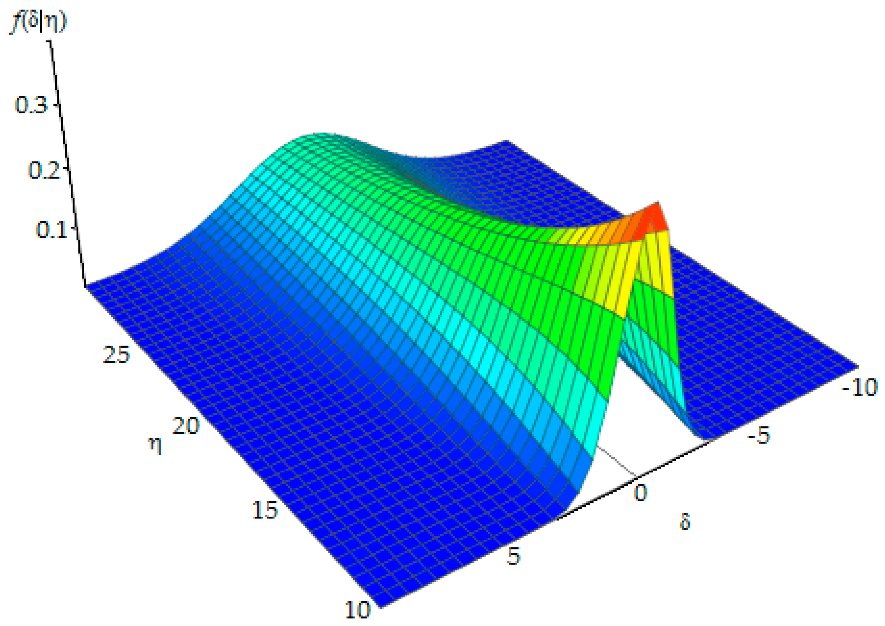
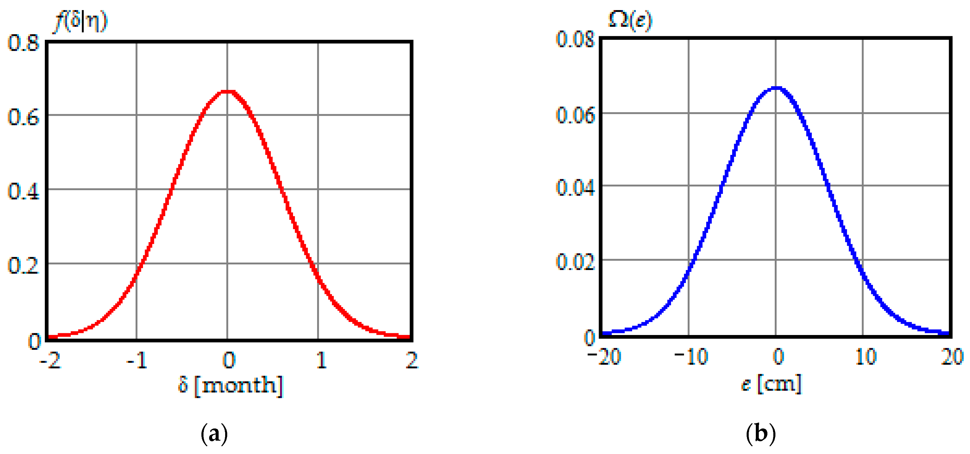
2. Quantification of the Uncertainty of Continuous Condition Monitoring

Let the state of the WT component be continuously monitored with the help of built-in sensors in the interval (0, τ), where τ is the periodicity of preventive maintenance. Further, we suppose that condition monitoring is imperfect, i.e., an operable WT component can be judged as inoperable at any instant of the interval (0, τ), and vice versa, an inoperable WT component can be judged as operable. We assume that a WT component is replaced at the time τ if the sensors do not indicate a failure during the interval (0, τ) or at any instant of the interval (0, τ), if at that instant the sensors indicate failure. Decisions made based on monitoring the condition of the WT component during the interval (0, τ) are reduced to conducting a preventive or corrective maintenance. After any type of maintenance, the WT component becomes as good as new. The trustworthiness of continuous condition monitoring results has a significant impact on these decisions.
Let us consider the graph of decision-making when monitoring the condition of a WT component in the interval (0, τ), which is shown in Figure 1. A priori, the WT component can be in the operable state in the interval (0, τ) with probability P(τ) or the inoperable state with probability 1 − P(τ). According to the results of continuous condition monitoring of the WT component in the interval (0, τ) one of the following events may occur. The component will not fail, and the sensors will not give an alarm (true positive—TP), the component will not fail, but the sensors will provide a warning (false positive—FP), the component will fail, and the sensors will alarm (true negative—TN), and finally the component will fail, but the sensors will not trigger an alarm (false negative—FN). The probabilities of these events are marked as P T P ( τ ) , P F P ( τ ) , P T N ( τ ) , and P F N ( τ ) in the graph of Figure 1.
It should be noted that the probabilities indicated in Figure 1 are determined on a time interval (0, τ) of continuous condition monitoring, i.e., these probabilities are interval probabilities, and do not correspond to some point in time.
Let us determine the probabilities of a TP, FP, TN, and FN in the interval (0, τ). Assume that the random variable H (H ≥ 0) denotes the time to failure of the WT component with a failure probability density function (PDF) ω(η). The random variable H is the smallest root of the stochastic equation
X ( t ) F T = 0 ,
where X(t) is the stochastic process of the WT component degradation and FT is the degradation failure threshold.
Since the sensors are assumed to be error-prone, the observed process Y(t) can be represented as the sum of the degradation processes X(t) and noise e(t).
Y ( t ) = X ( t ) + e ( t ) .
Let us consider the random variable H*, which is the smallest root of the stochastic equation
Y ( t ) F T = 0 .
The random variable H* is the occasional time until the stochastic process Y(t) crosses the failure threshold FT. Figure 2 illustrates the difference between the realizations x(t) and y(t) of the stochastic processes X(t) and Y(t), and realizations η and η* of the random variables H and H*. Equation (3) shows that random variable H* is a function of random variable H and noise e(t). That is why the realizations of time to failure η* and η do not match in Figure 2.
The presence of noise e(t) in Equation (3) leads to a random error in evaluation of time to failure, which is defined as follows:
Δ = Η Η .
Random variables H (0 < H < ∞) and Δ (−∞ < Δ < ∞) have an additive relationship. Therefore, the random variable H* is defined in a continuous range of values from −∞ to ∞.
Using the definitions of random variables H and H*, we formulate events related to FP, TP, FN, and TN during the interval (0, τ) as follows:
F P ( 0 , τ ) = [ ( Η τ ) ( Η τ ) ] ,
T P ( 0 , τ ) = [ ( Η τ ) ( Η τ ) ] ,
F N ( 0 , τ ) = [ ( Η τ ) ( Η τ ) ] ,
T N ( 0 , τ ) = [ ( Η τ ) ( Η τ ) ] .
The probabilities of events (5)–(8) can be found by calculating the probability of hitting a random point {H, H*} in a 2D domain created by the boundaries of variation of each random variable, and is equal to 2-fold integral over this area. Let us denote the joint PDF of the random variables {H, H*} as ω 0 ( η , η * ) . The event FP(0, τ) corresponds to the 2D domain with the following limits: τ Η < and < Η * τ . By integrating the PDF ω 0 ( η , η * ) within the specified region, we determine the probability of FP.
P F P ( 0 ,   τ ) = P [ F P ( 0 ,   τ ) ] = τ τ ω 0 ( η , η * ) d η * d η .
We derive the probabilities of events TP(0, τ), FN(0, τ), and TN(0, τ) analogically to the probability P F P ( 0 , τ ) . Conducting some mathematical manipulations we obtain
P T P ( 0 ,   τ ) = P [ T P ( 0 ,   τ ) ] = τ τ ω 0 ( η , η * ) d η * d η ,
P F N ( 0 ,   τ ) = P [ F N ( 0 ,   τ ) ] = 0 τ τ ω 0 ( η , η * ) d η * d η ,
P T N ( 0 ,   τ ) = P [ T N ( 0 ,   τ ) ] = 0 τ τ ω 0 ( η , η * ) d η * d η .
As can be seen from (9)–(12), in order to find the probabilities FP, TP, FN, and TN, the joint PDF ω 0 ( η , η * ) should be known. Let us present the joint PDF ω 0 ( η , η * ) as follows:
ω 0 ( η , η * ) = ω ( η ) θ ( η * | η ) ,
where θ ( η * | η ) is the conditional PDF of random variable Η * provided that Η = η .
From (4), when H = η, the random variable H* reduces to H* = η + Δ. Since between the random variables H and Δ exists the additive relationship, the following equality thus holds:
θ ( η * | η ) = f ( η * η | η ) ,
where f ( η * η | η ) is the conditional PDF of the random error in evaluation of time to failure, provided that H = η.
Substituting (14) into (13) gives
ω 0 ( η , η * ) = ω ( η ) f ( η * η | η ) .
The relation (15) makes it possible to simplify (9)–(12). By substitution of (15) into (9), we get
P F P ( 0 ,   τ ) = τ ω ( η ) τ f ( η * η | η ) d η * d η .
Making the substitution δ = η * η in the internal integral of (16) results in the following expression for FP:
P F P ( 0 ,   τ ) = τ ω ( η ) τ - η f ( δ | η ) d δ d η .
Accomplishing a similar change of variable in expressions (10)–(12), we get
P T P ( 0 ,   τ ) = τ ω ( η ) τ - η f ( δ | η ) d δ d η .
P F N ( 0 ,   τ ) = 0 τ ω ( η ) τ - η f ( δ | η ) d δ d η .
P T N ( 0 ,   τ ) = 0 τ ω ( η ) - τ - η f ( δ | η ) d δ d η .
As seen from (17)–(20), to calculate the probabilities of FP, TP, FN, and TN when performing continuous condition monitoring of a WT component, the PDF ω(η) and f ( δ | η ) are supposed to be known. We should also note that formulas (17)–(20) are generalized, i.e., they can be used for any stochastic degradation process X(t) and any noise e(t).

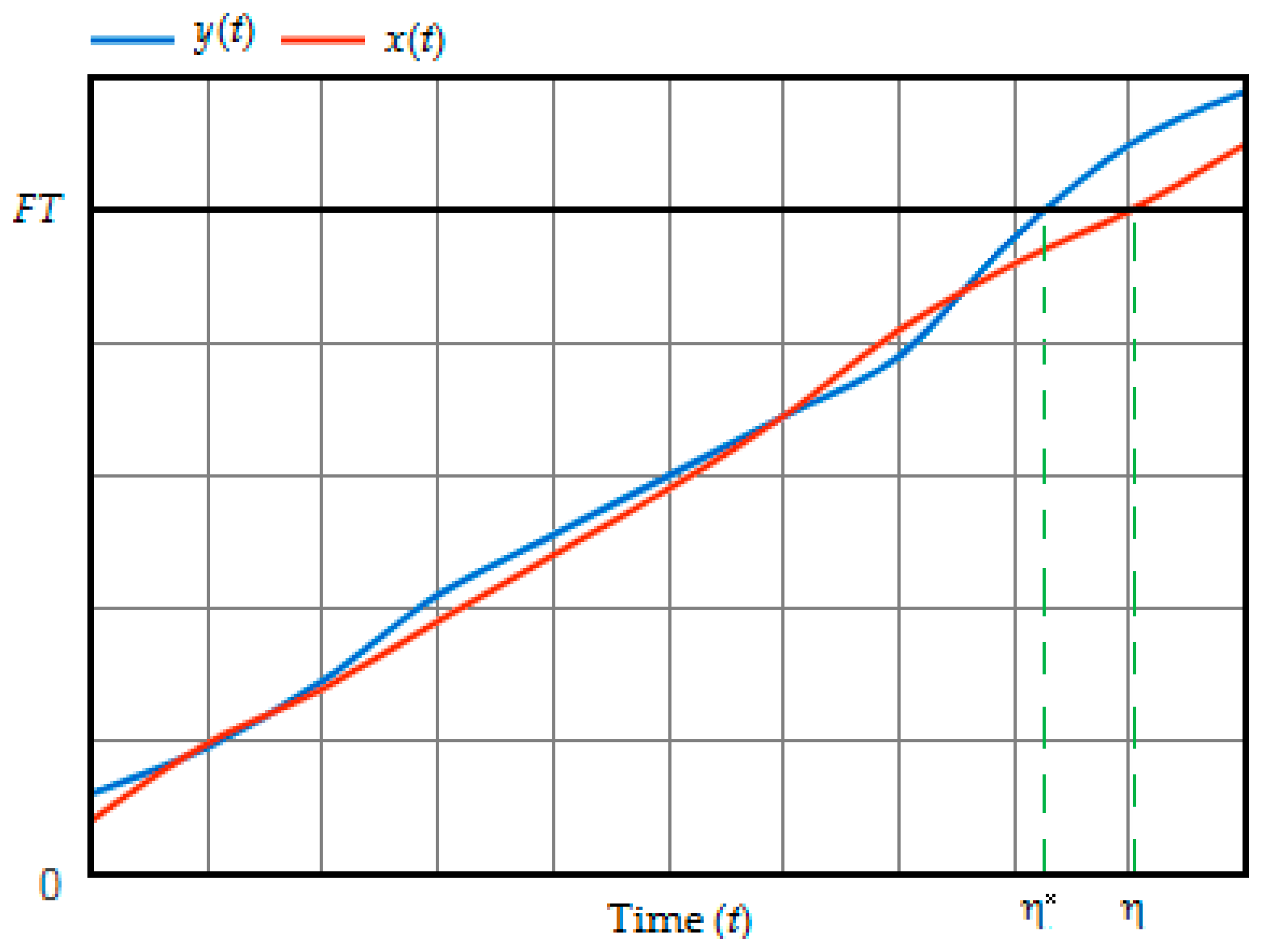
3. Maintenance Model with Imperfect Continuous Condition Monitoring

Let us consider the mathematical maintenance model of a WT component in the interval (0, τ) with imperfect continuous condition monitoring. Further, we consider the problem of minimizing the expected maintenance cost per unit of time of a WT component for an infinite time horizon. The decision to conduct a maintenance action on the WT component is based on information received from the sensors. The decision to conduct corrective maintenance within the interval (0, τ) is made in the case of failure detection, which corresponds to the occurrence of the TN(0, τ) event. In the case of the FP(0, τ) event occurring, the preventive maintenance is carried out. If the alarm signal does not appear in the interval (0, τ), it means that a TP(0, τ) event occurred, or that the component failed, and an FN(0, τ) event appeared. Since the time horizon is infinite, it is appropriate to choose the expected maintenance cost per unit of time as the maintenance effectiveness indicator of the WT component. Since after any type of maintenance, the WT component becomes as good as new, then according to the authors of [34], the expected cost of maintenance per unit of time can be determined as the ratio of the average maintenance cost for the regeneration cycle to the average duration of this cycle.
E [ C u ( τ ) ] = E [ C a ( τ ) ] E [ T R C ( τ ) ] .
The optimization problem is as follows:
τ o p t min τ E [ C u ( τ ) ] ,
where τ o p t is the optimal periodicity of preventive maintenance.
The average maintenance cost for one regeneration cycle consists of two parts. The first part determines the cost of maintenance for the case when a failure occurs in the interval (0, τ), i.e., Η τ . Let the failure occur at the moment Η = η τ . Then the cost of maintenance includes the cost of corrective repair if the sensors detect the failure, and the cost of losses due to unrevealed failure state of the WT component if the sensors do not identify the failure.
E [ C a ( τ ) | Η = η τ ] = C C M P T N ( η , τ | Η = η ) + C U F ( τ η ) P F N ( η , τ | Η = η ) ,
where C C M is the cost of corrective maintenance, C U F is the loss cost per unit of time due to unrevealed failure, P T N ( η , τ | Η = η ) is the conditional probability of TN in the interval (η, τ) provided that Η = η , and P F N ( η , τ | Η = η ) is the conditional probability of FN in the interval (η, τ) provided that Η = η .
Using (19) and (20) we determine the conditional probabilities P F N ( η , τ | Η = η ) and P T N ( η , τ | Η = η ) as follows:
P F N ( η , τ | Η = η ) = τ - η f ( z | η ) d z ,
P T N ( η , τ | Η = η ) = - τ - η f ( z | η ) d z .
The second part determines the cost of maintenance for the case when no failure occurs in the interval (0, τ), i.e., Η > τ . In this case, the cost of maintenance includes the cost of preventive maintenance, either if the sensors incorrectly detect a failure in the interval (0, τ), or if the sensors do not send an alarm signal in the interval (0, τ).
E [ C a ( τ ) | Η = η > τ ] = C P M F P P F P ( 0 , τ | Η = η ) + C P M T P P T P ( 0 , τ | Η = η ) ,
where C P M F P and C P M T P are, respectively, the cost of preventive maintenance due to the FP and TP events, P F P ( 0 , τ | Η = η ) is the conditional probability of FP in the interval (0, τ) provided that Η = η , and P T P ( 0 , τ | Η = η ) is the conditional probability of TP in the interval (0, τ) provided that Η = η .
The values of C P M F P and C P M T P may not match, because in the case of occurrence of FP, the preventive maintenance is unscheduled, and in the case of TP, the preventive maintenance is scheduled.
On the base of (17) and (18), we determine the conditional probabilities P F P ( 0 , τ | Η = η ) and P T P ( 0 , τ | Η = η )
P F P ( 0 , τ | Η = η ) = - τ - η f ( δ | η ) d δ ,
P T P ( 0 , τ | Η = η ) = τ - η f ( δ | η ) d δ .
Applying the law of total expectation, we determine the average maintenance cost for one regeneration cycle:
E [ C a ( τ ) ] = 0 τ E [ C a ( τ ) | Η = η τ ] ω ( η ) d η + τ E [ C a ( τ ) | Η = η > τ ] ω ( η ) d η .
Substituting (23) and (26) into (29) gives
E [ C a ( τ ) ] = C C M P T N ( 0 , τ ) + C U F 0 τ ( τ η ) P F N ( η , τ | Η = η ) ω ( η ) d η + C P M F P P F P ( 0 , τ ) + C P M T P P T P ( 0 , τ ) .
Let us now determine the mean time of the regeneration cycle. In deriving the expression for E [ T R C ( τ ) ] , we will consider that within the interval (0, τ), the maintenance is possible only due to the occurrence of either an FP event or a TN event. Assume that Η = η τ . Then, the conditional mathematical expectation of the regeneration cycle is
E [ T R C ( τ ) | Η = η τ ] = η P T N ( η , τ | Η = η ) + ( τ η ) P F N ( η , τ | Η = η ) .
Now suppose that Η = η > τ . In this case, we have
E [ T R C ( τ ) | Η = η > τ ] = 0 τ z ω F P ( z | η ) d z + τ P T P ( 0 , τ | Η = η ) ,
where ω F P ( z | η ) is the conditional PDF of an FP in the interval ( 0 ,   z ) ,   0 < z τ , provided that Η = η .
The conditional PDF ω F P ( z | η ) is a derivative of the cumulative distribution function of the time to a false alarm under condition that Η = η
ω F P ( z | η ) = d d z { z η f ( δ | η ) d δ } .
Using the theorem on the derivative of an integral by a variable upper limit, we find
ω F P ( z | η ) = f ( z - η | η ) .
Substituting (34) into (32) gives
E [ T R C ( τ ) | Η = η > τ ] = 0 τ z f ( z η | η ) d z + τ P T P ( 0 , τ | Η = η ) ,
Using the law of total expectation, we determine the mean time of the regeneration cycle:
E [ T R C ( τ ) ] = 0 τ E [ T R C ( τ ) | Η = η τ ] ω ( η ) d η + τ E [ T R C ( τ ) | Η = η > τ ] ω ( η ) d η .
By substitution of (31) and (35) into (36), we have
E [ T R C ( τ ) ] = 0 τ P T N ( η , τ | Η = η ) ω ( η ) d η + 0 τ ( τ η ) P F N ( η , τ | Η = η ) ω ( η ) d η + τ 0 τ f ( z η | η ) ω ( η ) d z d η + τ τ P T P ( 0 , τ | Η = η ) ω ( η ) d η .
For the case when the condition monitoring is perfect, Equation (37) reduces to
E [ T R C ( τ ) ] = 0 τ ω ( η ) d η + τ τ ω ( η ) d η ,
which coincides with the well-known expression [34].

4. Example: Preventive Maintenance of Wind Turbine Blades

4.1. Methods of Condition Monitoring of Wind Turbine Blades

Modern WT rotor blades are usually made of composite materials. Different types of damage may occur in WT blades. The most common damages to the WT rotor blades are as follows [36]: cracks along adhesive joints, cracks parallel to the fiber direction, cracks along the plane between plies, etc. The causes of the defects that appear in WT rotor blades are analyzed in many studies, for example [36,37,38,39]. Blade cracks can be detected by periodical visual inspections, periodical inspections on the base of nondestructive testing, or online condition monitoring using sensors. A detailed analysis of different testing, inspecting, and online monitoring technologies for WT blades and other components is described in [14,38,40,41]. As mentioned in many studies, online condition monitoring is a promising technique for reducing the maintenance cost and downtime of WT [42,43,44,45]. The online monitoring methods include the acoustic emission detection method, the thermal imaging method, the ultrasonic method, the fiber optics method, and some others [38]. According to the authors of [38], ultrasonic methods allow for the identification of cracks, several mm in size. Nowadays, optical fiber sensors are widely used in different structural health monitoring systems [46,47,48,49,50,51]. The use of an online monitoring system based on Brillouin optical time-domain analysis allows for detecting a crack as small as 1.5 cm, when monitoring a wind turbine blade [52].
Further, we assume that one of the methods, as mentioned above, is used for online condition monitoring of WT blade damages. Some forms of damage, once they have appeared in the composite blade structure, will quickly spread and may overload other structural components that finally may lead to a failure of the WT. The destruction of a WT blade usually leads to significant economic losses.

4.2. Crack Degradation Model

An increase in the size of the crack leads to a rise in the probability of failure of the WT blade. The dependence of the length of a growing crack on time is a monotonic function. In the general case, such a function is convex. The following random function can be used to approximate the monotonic stochastic process of crack degradation:
X ( t ) = A t γ ,
where A is the random degradation rate of crack [cm/unit of time] and γ is the exponent of time.
If γ > 1, then the realizations of the random function X(t) have a convex shape.
For calculating the average maintenance cost per unit of time we need to know the conditional PDF of random error in evaluating the time to failure f ( δ | η ) . Following the method described in [53], and assuming that the noise e(t) is a white noise, we derive the following equation for the PDF f ( δ | η ) :
f ( δ | η ) = γ ( F T η ) | ( δ + η η ) γ 1 | Ω { F T [ 1 ( δ + η η ) γ ] } ,
where Ω(e) is the PDF of the random measurement error.
For the sake of simplicity, assume that the crack degradation function is linear, i.e., γ = 1. In this case, from (40) we obtain
f ( δ | η ) = ( F T η ) Ω ( - F T η δ ) .
In the case when the measurement noise is Gaussian white noise, (41) transforms into the following equation:
f ( δ | η ) = ( 1 σ e 2 2 π ) ( F T η ) exp { 1 2 σ e 2 [ ( F T ) δ η ] 2 } ,
where σ e is the standard deviation of the measurement noise.
For a linear stochastic process of crack degradation, the PDF of the time to failure is given by [54]:
ω ( η ) = m 1 σ 1 2 η 2 + σ 1 2 η ( F T m 1 η ) 2 π σ 1 3 η 3 exp { ( F T m 1 η ) 2 2 σ 1 2 η 2 } ( 0 φ ( a ) d a ) 1 ,
where m 1 and σ 1 are the mathematical expectation and standard deviation of the random degradation rate of crack, and φ ( a ) is the Gaussian PDF of the random degradation rate of crack A   [ cm unit   of   time ] . The distribution of A is truncated because negative rates are impossible.
The crack can begin its growth at any time during the lifetime of the blade. Thus, for determining the average lifetime maintenance cost, the expected maintenance cost during the regeneration cycle of the blade should be multiplied by the crack initiation rate (θ), and the lifetime of a WT ( T L T ) .
E [ C L T ( τ ) ] = θ T L T E [ C a ( τ ) ] .

4.3. Model Parameters

In determining the optimal periodicity of preventive maintenance, we mostly use the initial data given in [25] for an offshore WT. As indicated in [25], even a small crack size of 20–30 mm for the delamination may reduce the strength of the blades, and may finally be a reason for failure. Further, we assume that FT = 60 cm. The cost of corrective maintenance due to catastrophic failure is C C M C F = 440 , 400 , which includes the cost of a new blade, the cost of production losses, the cost of ordering a boat and crane, and the cost of installation. The cost of ordering an offshore boat and inspection CM is assumed to be €12,500. The cost of corrective maintenance due to degradation failure is usually significantly less than C C M C F because the damaged blade can be repaired in situ. In calculations, we assume that C C M = 100 , 000 . Furthermore, it will be shown that, for a degrading component, a false alarm usually occurs when the value of the degradation parameter approaches the threshold FT. Based on this we assume that losses due to an FP will include the cost of ordering an offshore boat, the inspection cost, and the cost of in situ repair by patch technique because of advanced degradation. Therefore, we assume that C P M F P = 20 , 000 . The cost of preventive maintenance due to TP event at the end of the interval (0, τ), we assume to be equal C P M F P , i.e., C P M T P = 20 , 000 . The loss cost per unit of time due to unrevealed failure, we calculate assuming that, as in [25], the average power production is 2 MW and the price for electricity is 50 €/MWh. In this case, we calculate that C U F = 72 , 000   month . It should be noted that in 2018, the cost of electricity in Europe was significantly higher varying from 100.5 €/MWh in Bulgaria to 312.3 €/MWh in Denmark [55]. Following study [25], we assume that the crack initiation rate θ is in the range of 0.05–0.2 [1/year] and the lifetime T L T for one WT is 25 years.
Table 2 shows a summary of the model parameters.

5. Results and Discussion

This section of the article presents the results and discussion of the preventive maintenance optimization of WT blades on the basis of the mathematical model developed in Section 2 and Section 3.

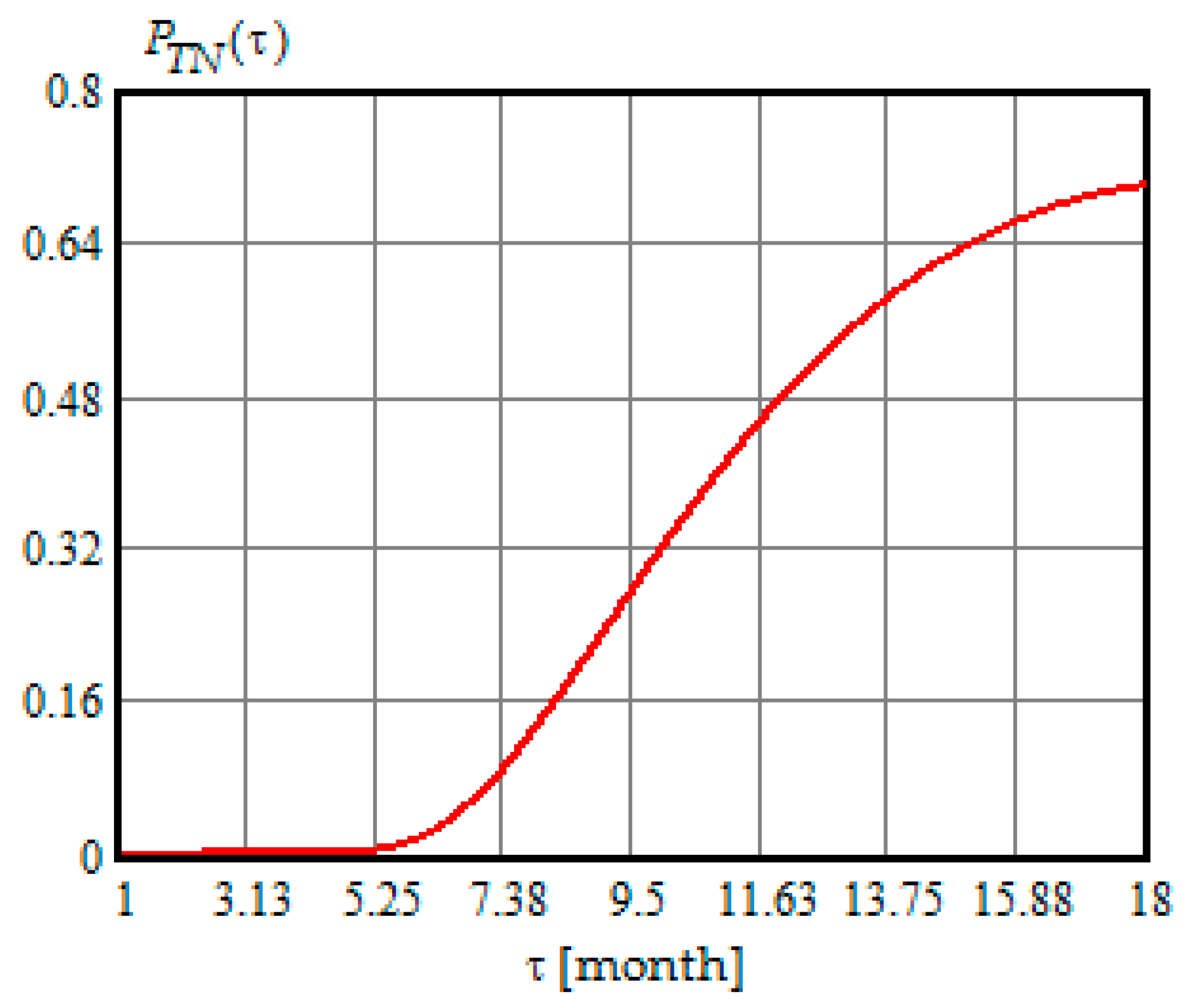
5.1. Investigation of Probabilities of Correct and Incorrect Decisions of Online Condition Monitoring

The probabilities of correct and incorrect decisions at the online condition monitoring of the WT blades are calculated using formulas (17)–(20). As can be seen from (17)–(20), to calculate these probabilities, PDF f ( δ | η ) and ω(η) should be known. Using expressions (42) and (43), let us investigate the behavior of PDF f ( δ | η ) and ω(η).
Figure 3 shows a 3D presentation of the conditional PDF f ( δ | η ) , plotted by 3D Surface Plotter when F T = 60   cm and σ e = 6   cm .
As can be seen in Figure 3, the conditional PDF f ( δ | η ) flattens with an increase in the failure time η, which indicates an increase in the variance of the error in evaluating the time to failure.
Figure 4a shows a plot for the conditional PDF of the measurement error in evaluating the time to failure when η = 6   months . As can be seen in Figure 4a, the PDF f ( δ | η ) has a symmetric Gaussian distribution. For comparison, Figure 4b shows a plot for the PDF of the measurement error Ω(e). By comparing the plots presented in Figure 4a and 4b, we can see that both PDFs are of the same form, though the abscissa axis denotes the error in evaluating the time to failure for the PDF f ( δ | η ) and the measurement error of sensors for the PDF Ω(e). Thus, the conditional PDF f ( δ | η ) allows the conversion of sensor errors into errors in evaluating the time to failure of a WT component. Essentially, this is the conversion of spatial characteristics (errors of sensors) into temporary characteristics (errors in evaluating the time to failure). Knowledge of PDF f ( δ | η ) allows for calculating the probabilities of the events FP, TP, FN, and TN during any interval of condition monitoring.
Figure 5a shows the plot of the PDF ω ( η ) when m 1 = 5   cm month , σ 1 = 2.5   cm month , and F T = 60   cm . As can be seen in Figure 5, PDF ω(η) begins to grow sharply at η = 4.4   months and reaches a maximum at η = 8.9   months .
Figure 5b shows the dependence of the probability of failure Q(η) as a function of time to failure. As can be seen from Figure 5b, the probability of failure reaches 10% at η = 5.6 months, 25% at η = 8.9 months, and 50% at η = 12 months. From the graph in Figure 5b, we can see that the highest increase in the probability of failure falls on the time interval of 5–12 months.
Figure 6, Figure 7, Figure 8 and Figure 9 show the dependence of the probabilities of a FP, TP, FN, and TN on the length of the monitoring interval τ when σ e = 6   cm and the rest of data are the same as for Figure 5.
From the analysis of dependencies in Figure 6, Figure 7, Figure 8 and Figure 9, we can draw the following conclusions:
  • All probabilities depend on the length of the monitoring interval τ;
  • The probability of an FP begins to go up remarkably at τ = 4 months and gets to 3.8% at τ = 9.5 months, and then slowly decreases to 1.6 % at τ = 18 months;
  • The probability of TP decreases slowly, reaching 98.5% at τ = 4.75 months, and then begins to decrease rapidly, reaching 22.4% at τ = 18 months;
  • The probability of FN begins to increase remarkably at τ = 5.25 months reaching the maximum value of 3.4% in the vicinity of the maximum of PDF of time to failure when τ = 10.6 months, and then decreases reaching 1.8% at τ = 18 months;
  • The probability of TN begins to increase significantly at τ = 5.5 months when its value is 0.7%, and then increases sharply reaching 74.2% at τ = 18 months.
The behavior of the curves in Figure 6, Figure 7, Figure 8 and Figure 9 requires some explanation. The dependence of P F P ( τ ) in Figure 6 is explained by the behavior of the sum of the crack size and sensor noise according to Equation (2). When the crack size is small and far from the FT threshold, the probability that the sum of the crack size and sensor noise exceeds the threshold FT is low. That is why for small crack size, the probability of a false alarm is negligible. However, as the mathematical expectation of the crack size approaches the FT threshold, the probability that the sum of the crack size and noise exceeds the threshold FT increases. Therefore, the probability of a false alarm also increases, reaching a maximum at τ = 9.5 months. When the mathematical expectation of the crack size exceeds the FT threshold, the probability of a false alarm decreases, because most probably, the unit failed, and as is well-known, the false alarms occur only for operable units.
Let us explain the dependence of P T P ( τ ) in Figure 7. When the crack size is small and far from the FT threshold, the probability that the sum of the crack size and sensor noise is less than the threshold FT is high. That is why, for small crack size, the probability of a TP event is high. However, as the crack size rises toward FT threshold, the probability that the sum of the crack size and noise is less than the threshold FT decreases. Therefore, the probability of a TP also decreases, reaching 22.4% at τ = 18 months.
The dependence of P F N ( τ ) in Figure 8 is also explained by the behavior of the sum of the crack size and sensor noise in respect to the threshold FT. When the crack size is small and far from the FT threshold, the probability of failure is also small, according to Figure 5b. That is why the probability that the crack size exceeds FT threshold, and that the sum of the crack size and sensor noise is less than the threshold FT, is shallow. Therefore, for small crack size, the probability of an FN is negligible. Beginning from τ = 5.25 months the probability of failure increases remarkably, which means that an increasing number of realizations of the stochastic process X(t) exceed the threshold FT. However, for some of these realizations, the sum of the crack size and noise is less than the threshold FT, which leads to false-negative events. The probability of an FN reaches the maximum at τ = 10.6 months where the increase in the probability of failure is the maximum. When the mathematical expectation of the crack size moves up from the FT threshold, the probability of an FN decreases because it is unlikely that the sum of the crack size and sensor noise will be less than the threshold FT.
The dependence of P T N ( τ ) in Figure 9 is opposite to that in Figure 7. When the crack size is small and far from the FT threshold, the probability that the sum of the crack size and sensor noise exceeds the threshold FT is low. That is why, for small crack size, the probability of a TN event is also low. However, as the crack size rises, the probability that the sum of the crack size and noise is higher than the threshold FT increases. Therefore, the probability of a TN also increases, reaching 74.2% at τ = 18 months.
Thus, from the conducted numerical analysis of the behavior of the probabilities of correct and incorrect decisions when continuously monitoring the condition of the blades, it follows that these probabilities are not constant in time and should be considered when optimizing the periodicity of preventive maintenance.
It should be noted that in the maintenance models with periodic condition monitoring, the probabilities of an FP, TP, FN, and TN are considered in many studies, for example [56,57,58,59]. However, in these mathematical models, the authors assumed that the probabilities of correct and incorrect decisions had constant values and do not depend on time and parameters of the degradation process.

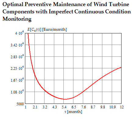
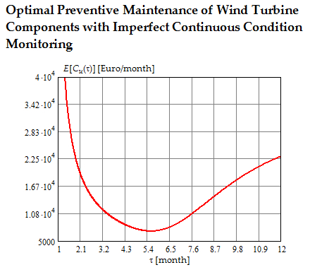
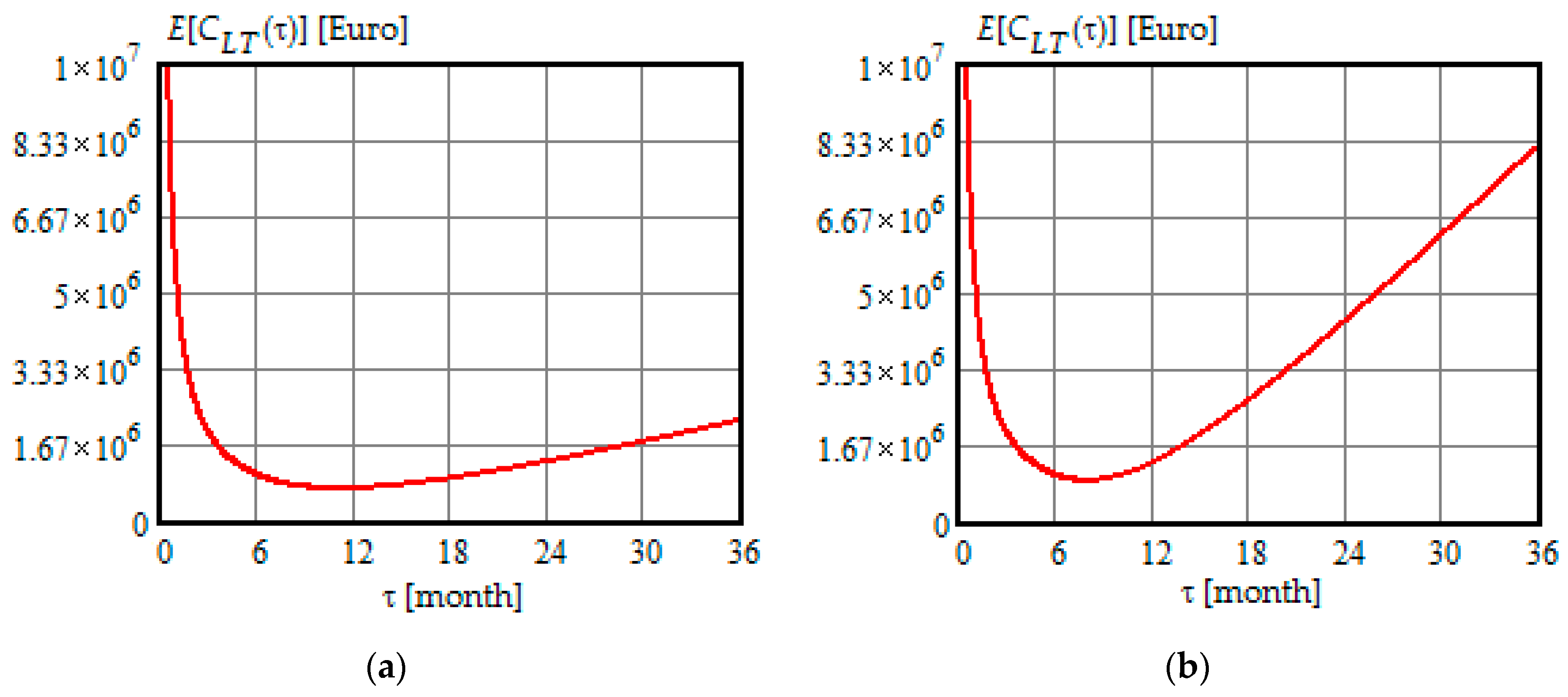
5.2. Investigation of the Expected Cost of Preventive Maintenance with Online Condition Monitoring

Figure 10 shows the dependence of the expected maintenance cost per unit of time on the periodicity of preventive maintenance for the data given in Table 2.
As can be seen in Figure 10, the expected cost of maintenance per unit of time is a convex function of the periodicity of preventive maintenance τ. When τ is small, the expected maintenance cost is too high due to frequently conducted preventive maintenance. When τ is large, the expected maintenance cost is also high due to dominated corrective maintenance cost C C M , which is significantly higher than preventive maintenance cost C P M T P . Optimal periodicity of preventive maintenance ensures the minimal expected cost of maintenance per unit of time, providing a trade-off between the weighted cost of preventive and corrective maintenance. Indeed, at the optimal periodicity of 6 months, the expected maintenance cost per unit of time is minimal and equal to 3600 / month .
The obtained result requires clarification. Modern WT are usually designed to work for 20–25 years [41,60]. Therefore, the optimal periodicity of preventive maintenance refers to the case of a crack occurrence and its further growth in the WT blade. Calculating (30) for the data given in Table 2, we obtain that the average maintenance cost E [ C a ( τ ) ] for one regeneration cycle is €21,230. Substituting θ and T L T from Table 2, and E [ C a ( τ ) ] into (44) we calculate that the range of the average lifetime maintenance cost for one WT blade is €26,540 to €106,160 depending on the crack initiation rate.
Let us compare preventive maintenance with online condition monitoring and predetermined preventive maintenance without condition monitoring. With online condition monitoring, preventive maintenance is only performed if a crack in the WT blade occurs and develops. If there is no crack, then only online condition monitoring is performed. In the absence of an online condition monitoring system, preventive maintenance should be carried out after a specified time interval, regardless of whether there is a crack or not. Independently of the type of preventive maintenance, corrective maintenance is accomplished after the failure occurrence.
A mathematical model of the predetermined preventive maintenance of WT blades is given in Appendix A. Figure 11 shows the dependence of the lifetime maintenance cost on the periodicity of preventive maintenance.
From Figure 11, we can draw the following conclusions:
  • The average lifetime maintenance cost is a convex function of the periodicity of predetermined preventive maintenance;
  • The optimal periodicity of predetermined preventive maintenance decreases from 11 months to 8 months, when the crack initiation rate increases from 0.05 [1/year] to 0.2 [1/year];
  • The minimal value of the average lifetime maintenance cost increases with an increase in the crack initiation rate. Indeed, when θ = 0.05 [1/year], then E [ C L T ( τ ) ] = 687 , 200 ; when θ = 0.2 [1/year], then E [ C L T ( τ ) ] = 878 , 500 .
Comparing the results of calculations for preventive maintenance with online condition monitoring and without it, we note that when using condition monitoring, the maintenance cost is many times less (25.9 and 8.3, depending on θ). The reason for this is the fact that with online monitoring, preventive maintenance of the blades is carried out in the presence of a crack. Without condition monitoring, preventive maintenance is carried out after each interval τ, regardless of whether there is a crack or not.
The plots in Figure 11a,b match the case when the failure is unrevealed and C U F > 0 . Let us evaluate the average lifetime maintenance cost assuming that the failure is revealed, i.e., C U F = 0 . Figure 12a,b show the corresponding plots.
As can be seen in Figure 12a,b, over the interval (0, 8) months, the cost function decreases sharply, and with τ > 8 months, the average lifetime maintenance cost slowly decreases reaching at τ = 60 months the values of €196,700 and €486,800 with θ = 0.05 [1/year] and θ = 0.2 [1/year], respectively.
It should be noted that when using corrective maintenance without condition monitoring and C C M C F = 440 , 000 the average lifetime maintenance cost is €550,000 for θ = 0.05 [1/year] and €2,200,000 when θ = 0.2 [1/year].
Table 3 shows a summary of the average lifetime cost calculations for different maintenance types for WT blades.
From the analysis of Table 3, it follows that for any crack initiation rate, when using corrective or predetermined preventive maintenance, the average lifetime maintenance cost is many times higher than when using preventive maintenance with online condition monitoring.
In the numerical example, for simplicity, we assumed that the crack propagation model is linear. If the crack propagation function is not linear, in this case, Equations (1)–(38) are valid for any stochastic process of crack degradation and any measurement noise. The conditional PDF (40) is valid for any stochastic degradation process that can be represented by the model (39). The PDF (42) and (43) can be used only for the linear degradation model. The PDF of time to failure corresponding to the nonlinear model of degradation (39), i.e., in the case when γ > 1, is given in [54]. It should be noted once again that the proposed approach to optimizing preventive maintenance based on continuous condition monitoring is not limited to the model of the degradation process (39). Equations (1)–(38) can be used for any model of a stochastic degradation process. For example, there is a variety of stochastic processes suitable for the description of crack growth. We can mention here the stochastic gamma process for modeling gradual damage monotonically accumulating over time [61,62] and a class of increasing Markov processes [63,64].

6. Conclusions

This article has proposed a new approach to optimizing preventive maintenance with online condition monitoring, which assumes that the built-in sensors are error-prone and based on the information they provide, incorrect decisions when determining the condition of the WT component are possible. A mathematical model has been proposed to evaluate the probabilities of correct and incorrect decisions made on the results of continuous condition monitoring the deteriorating components of WT. Significantly, the article first has solved the problem of interval evaluation of probabilities of such events as false positive, true positive, false negative, and true negative for the case of continuous condition monitoring. It has been shown that probabilities of correct and incorrect decisions depend on the interval of continuous condition monitoring and are functions of the parameters of the degradation model. Furthermore, the probabilities of a false positive, true positive, false negative, and true negative have been incorporated into the mathematical model of preventive maintenance with continuous condition monitoring allowing to determine the average maintenance cost for one regeneration cycle, the mean time of the regeneration cycle, the expected maintenance cost per unit of time, and the average lifetime maintenance cost. The proposed mathematical equations for the expected cost of preventive maintenance with online condition monitoring are valid for any stochastic deterioration process and any measurement noise. The developed mathematical model has been examined on an example of optimizing the preventive maintenance of WT blades. By numerical calculations, it has been shown that with the optimal periodicity of preventive maintenance of 6 months the expected maintenance cost per unit of time is around 3600 Euro/month; the average maintenance cost for one regeneration cycle is €21,230; and the average lifetime maintenance cost for one WT blade is €26,540 to €106,160 for the lifetime of 25 years and at the crack initiation rate lying in the range of 0.05–0.2 [1/year]. It has also been shown that optimal preventative maintenance with online condition monitoring reduces the average lifetime maintenance cost by 11.8 times compared with corrective maintenance without condition monitoring, and by at least 4.2 and 2.6 times compared with predetermined preventive maintenance for low and high crack initiation rates, respectively.
The proposed mathematical model of preventive maintenance based on imperfect online condition monitoring can be used for a wide range of deteriorating systems since the basic equations do not limit the type of stochastic degradation process and the type of measurement noise.
Our future work will include an investigation of preventive maintenance of WT blades for the case of the nonlinear stochastic process of crack propagation; application of the developed mathematical model to some other components of WT; modification of the proposed maintenance model for case of a minimal repair policy; and development of a predictive maintenance model of WT components based on imperfect continuous monitoring.

Author Contributions

This article presents the collective work of two authors. The authors (A.R. and V.U.) jointly participated in the conceptualization of the problem, development of mathematical models, numerical calculations, and writing the article.

Funding

This research received no external funding.

Conflicts of Interest

The authors declare no conflict of interest.

Abbreviations

The following abbreviations exist in the manuscript:
CBMCondition-based maintenance
FNFalse negative
FPFalse positive
GWGigawatt
kwhKilowatt hour
MWMegawatt
MWhMegawatt hour
O&MOperation and maintenance
PDFProbability density function
TNTrue negative
TPTrue positive
WTWind turbine

Nomenclature

Hrandom time to failure of a WT component
ω(η)probability density function of time to failure
Q(η)probability of failure
τperiodicity of preventive maintenance
X(t)stochastic process of a WT component degradation
e(t)stochastic process of noise
Y(t)sum of stochastic processes X(t) and Y(t)
FTdegradation failure threshold
H*random time until stochastic process Y(t) crosses failure threshold FT
Δrandom error in evaluation of time to failure
ω 0 ( η , η * ) joint probability density function of random variables H and H*
P(τ)probability of failure-free operation of the WT component in the interval (0, τ)
FP(0, τ)a false positive event in the interval (0, τ)
TP(0, τ)a true positive event in the interval (0, τ)
FN(0, τ)a false negative event in the interval (0, τ)
TN(0, τ)a true negative event in the interval (0, τ)
P F P ( 0 , τ ) probability of a false positive in the interval (0, τ)
P T P ( 0 , τ ) probability of a true positive in the interval (0, τ)
P F N ( 0 , τ ) probability of a false negative in the interval (0, τ)
P T N ( 0 , τ ) probability of a true negative in the interval (0, τ)
θ ( η * | η ) conditional probability density function of random variable Η *
f ( δ | η ) conditional probability density function of the random error in evaluation of time to failure
E [ C a ( τ ) ] average maintenance cost for the time between renewals
E [ T R C ( τ ) ] average duration of the time between renewals (regeneration cycle)
E [ C u ( τ ) ] expected cost of maintenance per unit of time
τ o p t optimal periodicity of preventive maintenance
C C M cost of corrective maintenance due to degradation failure
C C M C F cost of corrective maintenance due to catastrophic failure
C U F loss cost per unit of time due to unrevealed failure
C P M F P cost of preventive maintenance due to false positive
C P M T P cost of preventive maintenance due to true positive
Ω(e)probability density function of the sensor random measurement error
σ e standard deviation of the measurement noise
m 1 mathematical expectation of the random degradation rate of crack
σ 1 standard deviation of the random degradation rate of crack
Arandom degradation rate of crack
γexponent of time
φ ( a ) Gaussian probability density function of the random degradation rate of crack
θcrack initiation rate
T L T lifetime of a WT
C M cost of ordering an offshore boat and inspection

Appendix A

In the case of predetermined preventive maintenance, the average maintenance cost for the time between renewals includes the expected cost due to corrective maintenance, preventive maintenance and the losses due to unrevealed failure, i.e.,
E [ C a ( τ ) ] = C C M 0 τ ω ( η ) d η + C U F 0 τ ( τ η ) ω ( η ) d η + C P M T P τ ω ( η ) d η ,
where 0 < τ θ 1 .
If C U F = 0 in (A1), we obtain well-known formula in age replacement model [34].
If the predetermined preventive maintenance is carried out with periodicity τ, then the total number of preventive maintenance cycles over the WT lifetime is
N = T L T τ .
The average number of cracks in the WT blade during the service life is determined as the product of the crack initiation rate and the lifetime, i.e.
n c r a c k = θ T L T .
Based on (A1)–(A3), the average lifetime maintenance cost is given by
E [ C L T ( τ ) ] = n c r a c k E [ C a ( τ ) ] + ( N n c r a c k ) C M ,
where C M is the cost of maintenance actions including ordering an offshore boat and inspection.
As seen from (A4), the average lifetime maintenance cost includes the cost of maintenance in the presence of a crack and the cost of maintenance in its absence. If a crack appeared in each maintenance interval τ, then τ = θ 1 , N = n c r a c k and the second term in (A4) would be zero.

References

  1. Wind Power Capacity Worldwide Reaches 597 GW, 50.1 GW Added in 2018. Available online: https://wwindea.org/blog/2019/02/25/wind-power-capacity-worldwide-reaches-600-gw-539-gw-added-in-2018/ (accessed on 25 February 2019).
  2. Renewable Power Generation Costs in 2017. Available online: https://www.irena.org/-/media/Files/IRENA/Agency/Publication/2018/Jan/IRENA_2017_Power_Costs_2018.pdf (accessed on 8 January 2018).
  3. Wind Turbine Maintenance Costs to Almost Double by 2020. Available online: https://www.edie.net/news/6/Win-turbine-maintenance-costs-to-nearly-doubl/ (accessed on 19 March 2015).
  4. Byon, E.; Ntaimo, L.; Ding, Y. Optimal maintenance strategies for wind turbine systems under stochastic weather conditions. IEEE Trans. Reliab. 2010, 59, 393–404. [Google Scholar] [CrossRef]
  5. Wind Farms: Preventive to Predictive Maintenance with Remote Monitoring. Available online: https://innovate.ieee.org/innovation-spotlight/wind-farm-preventive-maintenance-local-control-unit/ (accessed on 30 March 2017).
  6. Yildirim, M.; Gebraeel, N.Z.; Sun, X.A. Integrated predictive analytics and optimization for opportunistic maintenance and operations in wind farms. IEEE Trans. Power Syst. 2017, 32, 4319–4328. [Google Scholar] [CrossRef]
  7. Ouyang, T.; Yusen He, Y.; Huang, H. Monitoring wind turbines’ unhealthy status: A data-driven approach. IEEE Trans. Emerg. Top. Comput. Intell. 2019, 3, 163–172. [Google Scholar] [CrossRef]
  8. Huang, L.L.; Fu, Y.; Mi, Y.; Cao, J.L.; Wang, P. A Markov-chain-based availability model of offshore wind turbine considering accessibility problems. IEEE Trans. Sustain. Energy 2017, 8, 1592–1600. [Google Scholar] [CrossRef]
  9. Leonardi, F.; Messina, F.; Santoro, C. A risk-based approach to automate preventive maintenance tasks generation by exploiting autonomous robot inspections in wind farms. IEEE Access 2019, 7, 49568–49579. [Google Scholar] [CrossRef]
  10. Besnard, F.; Fischer, K.; Tjernberg, L.B. A model for the optimization of the maintenance support organization for offshore wind farms. IEEE Trans. Sustain. Energy 2013, 4, 443–450. [Google Scholar] [CrossRef]
  11. BS EN 13306: 2017. Maintenance—Maintenance Terminology. Available online: https://shop.bsigroup.com/ProductDetail/?pid=000000000030324472 (accessed on 1 December 2017).
  12. Artigao, E.; Martín-Martíneza, S.; Honrubia-Escribano, A.; Gómez-Lázaro, E. Wind turbine reliability: A comprehensive review towards effective condition monitoring development. Appl. Energy 2018, 228, 1569–1583. [Google Scholar] [CrossRef]
  13. Yang, B.; Dongbai, S. Testing, inspecting and monitoring technologies for wind turbine blades: A survey. Renew. Sustain. Energy Rev. 2013, 22, 515–526. [Google Scholar] [CrossRef]
  14. Stetco, A.; Dinmohammadi, F.; Zhao, X.; Robu, V.; Flynn, D.; Barnes, M.; Keane, J.; Nenadic, G. Machine learning methods for wind turbine condition monitoring: A review. Renew. Energy 2019, 133, 620–635. [Google Scholar] [CrossRef]
  15. Kang, J.; Jose Sobral, J.; Soares, C.G. Review of Condition-Based Maintenance Strategies for Offshore Wind Energy. J. Mar. Sci. Appl. 2019, 18, 1–16. [Google Scholar] [CrossRef]
  16. Sensor Solutions for Predictive Maintenance of Wind Turbines and Generators. Available online: https://www.micro-epsilon.co.uk/news/2019/2019-04-09-ME334-Sensor-solutions-for-predictive-maintenance-of-wind-turbines-and-generators/ (accessed on 9 May 2019).
  17. Canizo, M.; Onieva, E.; Conde, A.; Charramendieta, S.; Trujillo, S. Real-time predictive maintenance for wind turbines using big data frameworks. In Proceedings of the 2017 IEEE International Conference on Prognostics and Health Management (ICPHM), Dallas, TX, USA, 19–21 June 2017; pp. 1–8. [Google Scholar]
  18. Fu, Z.; Luo, Y.; Gu, C.; Li, F.; Yue, Y. Reliability analysis of condition monitoring network of wind turbine blade based on wireless sensor networks. IEEE Trans. Sustain. Energy 2019, 10, 549–557. [Google Scholar] [CrossRef]
  19. Krishna, D.G. Preventive maintenance of wind turbines using remote instrument monitoring system. In Proceedings of the 2012 IEEE Fifth Power India Conference, Murthal, India, 19–22 December 2012; pp. 1–5. [Google Scholar]
  20. Nilsson, J.; Bertling, L. Maintenance management of wind power systems using condition monitoring systems-life cycle cost analysis for two case studies. IEEE Trans. Energy Convers. 2007, 22, 223–229. [Google Scholar] [CrossRef]
  21. Kerres, B.; Fischer, K.; Madlener, R. Economic Evaluation of maintenance strategies for wind turbines: A stochastic analysis. IET Renew. Power Gener. 2015, 9, 766–774. [Google Scholar] [CrossRef]
  22. Van Horenbeek, A.; Van Ostaeyen, J.; Duflou, J.R.; Pintelon, L. Quantifying the added value of an imperfectly performing condition monitoring system—application to a wind turbine gearbox. Reliab. Eng. Syst. Saf. 2013, 111, 45–57. [Google Scholar] [CrossRef]
  23. Kaiser, K.A.; Gebraeel, N.Z. Predictive maintenance management using sensor-based degradation models. IEEE Trans. Syst. Man Cybern. Part A Syst. Hum. 2009, 39, 840–849. [Google Scholar] [CrossRef]
  24. Bryant, L.; John, A. Modelling wind turbine degradation and maintenance. Wind Energy 2016, 19, 571–591. [Google Scholar]
  25. Besnard, F.; Bertling, L. An approach for condition-based maintenance optimization applied to wind turbine blades. IEEE Trans. Sustain. Energy 2010, 1, 77–83. [Google Scholar] [CrossRef]
  26. Pattison, D.; Segovia Garcia, M.; Xie, W.; Quail, F.; Revie, M.; Whitfield, R.I.; Irvine, I. Intelligent integrated maintenance for wind power generation. Wind Energy 2016, 19, 547–562. [Google Scholar] [CrossRef]
  27. Ghamlouch, H.; Fouladirad, M.; Grall, A. The use of real option in condition-based maintenance scheduling for wind turbines with production and deterioration uncertainties. Reliab. Eng. Syst. Saf. 2019, 188, 614–623. [Google Scholar] [CrossRef]
  28. Shafiee, M.; Finkelstein, M. A proactive group maintenance policy for continuously monitored deteriorating systems: Application to offshore wind turbines. Proc. Inst. Mech. Eng. Part O J. Risk Reliab. 2015, 229, 373–384. [Google Scholar] [CrossRef]
  29. Shafiee, M.; Finkelstein, M.; Bérenguer, C. An opportunistic condition-based maintenance policy for offshore wind turbine blades subjected to degradation and environmental shocks. Reliab. Eng. Syst. Saf. 2015, 142, 463–471. [Google Scholar] [CrossRef]
  30. Wang, J.; Liang, Y.; Zheng, Y.; Gao, R.X.; Zhang, F. An integrated fault diagnosis and prognosis approach for predictive maintenance of wind turbine bearing with limited samples. Renew. Energy 2019, 142, 642–650. [Google Scholar] [CrossRef]
  31. Marugán, A.P.; Chacon, A.M.; Marquez, F.P. Reliability analysis of detecting false alarms that employ neural networks: A real case study on wind turbines. Reliab. Eng. Syst. Saf. 2019, 191, 106574. [Google Scholar] [CrossRef] [Green Version]
  32. Gertsbakh, I. Reliability Theory: With Applications to Preventive Maintenance; Springer: New York, NY, USA, 2001; pp. 84–89. [Google Scholar]
  33. Nakagawa, T. Replacement and preventive maintenance models. In Handbook of Performability Engineering; Misra, K.B., Ed.; Springer: London, UK, 2008; pp. 807–823. [Google Scholar]
  34. Nakagawa, T. Maintenance Theory of Reliability; Springer: London, UK, 2005; pp. 220–224. [Google Scholar]
  35. Kavaz, A.G.; Barutcu, B. Fault detection of wind turbine sensors using artificial neural networks. J. Sens. 2018, 2018, 5628429. [Google Scholar] [CrossRef]
  36. McGugan, M.; Pereira, G.; Sørensen, B.F.; Toftegaard, H.; Branner, K. Damage tolerance and structural monitoring for wind turbine blades. Philos. Trans. Royal Soc. A. Math. Phys. Eng. Sci. 2015, 373, 1–16. [Google Scholar] [CrossRef]
  37. Shokrieh, M.M.; Rafiee, R. Simulation of fatigue failure in a full composite wind turbine blade. Compos. Struct. 2006, 74, 332–342. [Google Scholar] [CrossRef]
  38. Cian, C.C.; Lee, J.R.; Bang, H.J. Structural health monitoring for a wind turbine system: A review of damage detection method. Meas. Sci. Technol. 2008, 19, 1–20. [Google Scholar]
  39. Wedel-Heinen, J.; Hayman, B.; Bronsted, P. Materials challenges in present and future wind energy. Mater. Res. Soc. Bull. 2008, 33, 343–354. [Google Scholar]
  40. Li, D.; Ho SC, M.; Song, G.; Ren, L.; Li, H. A review of damage detection methods for wind turbine blades. Smart Mater. Struct. 2015, 24, 1–24. [Google Scholar] [CrossRef]
  41. Hameed, Z.; Hong, Y.S.; Cho, Y.M.; Ahn, S.H.; Song, C.K. Condition monitoring and fault detection of wind turbines and related algorithms: A review. Renew. Sustain. Energy Rev. 2009, 13, 1–39. [Google Scholar] [CrossRef]
  42. Hyers, R.W.; McGowan, J.G.; Sullivan, K.L.; Manwell, J.F.; Syrett, B.C. Condition monitoring and prognosis of utility scale wind turbines. Energy Mater. 2006, 1, 187–203. [Google Scholar] [CrossRef]
  43. García, F.P.; Tobias, A.M.; Pinar, J.M.; Papaelias, M. Condition monitoring of wind turbines: Techniques and methods. Renew. Energy 2012, 46, 169–178. [Google Scholar] [CrossRef]
  44. Lu, B.; Li, Y.; Xin Wu, X. A Review of Recent Advances in Wind Turbine Condition Monitoring and Fault Diagnosis. In Proceedings of the 2009 IEEE Power Electronics and Machines in Wind Applications, Lincoln, NE, USA, 24–26 June 2009; pp. 1–7. [Google Scholar]
  45. Wang, K.; Sharma, V.S.; Zhang, Z.Y. SCADA data based condition monitoring of wind turbines. Adv. Manuf. 2014, 2, 61–69. [Google Scholar] [CrossRef] [Green Version]
  46. Lopez-Higuera, J.M.; Rodriguez, L.; Quintela, A.; Cobo, A.; Madruga, F.J.; Conde, O.M.; Lomer, M.; Quintela, M.A.; Mirapeix, J. Fiber optics in structural health monitoring. In Advanced Sensor Systems and Applications IV; Brian, G., Ed.; Curran Associates, Inc.: Red Hook, NY, USA, 2010. [Google Scholar]
  47. Güemes, A.; Fernández-López, A.; Díaz-Maroto, P.F. Structural health monitoring in composite structures by fiber-optic sensors. Sensors 2018, 18, 1094. [Google Scholar] [CrossRef] [PubMed]
  48. Murayama, H.; Wada, D.; Igawa, H. Structural health monitoring by using fiber-optic distributed strain sensors with high spatial resolution. Photonic Sens. 2013, 3, 355–376. [Google Scholar] [CrossRef] [Green Version]
  49. Jaaskelainen, M. Fiber Optic Distributed Sensing Applications in Defense, Security, and Energy; Udd, E., Du, H.H., Wang, A., Eds.; SPIE: Orlando, FL, USA, 2009; p. 731606. [Google Scholar]
  50. Mishnaevsky, L.; Branner, K.; Petersen, H.; Beauson, J.; McGugan, M.; Sørensen, B. Materials for wind turbine blades: An overview. Materials 2017, 10, 1285. [Google Scholar] [CrossRef]
  51. Oh, K.Y.; Park, J.Y.; Lee, J.S.; Epureanu, B.I.; Lee, J.K. A novel method and its field tests for monitoring and diagnosing blade health for wind turbines. IEEE Trans. Instrum. Meas. 2015, 64, 1726–1733. [Google Scholar] [CrossRef]
  52. Zhang, F.; Li, Y.; Yang, Z.; Zhang, L. Investigation of wind turbine blade monitoring based on optical fiber Brillouin sensor. In Proceedings of the 2009 International Conference on Sustainable Power Generation and Supply, Nanjing, China, 6–7 April 2009; pp. 1–4. [Google Scholar]
  53. Raza, A.; Ulansky, V. Modelling of predictive maintenance for a periodically inspected system. Procedia CIRP 2017, 59, 95–101. [Google Scholar] [CrossRef]
  54. Ignatov, V.A.; Ulansky, V.V.; Taisir, T. Prediction of Optimal Maintenance of Technical Systems; Znanie: Kiev, Ukraine, 1981; pp. 9–10. (In Russian) [Google Scholar]
  55. Electricity Price Statistics. Available online: https://ec.europa.eu/eurostat/statistics-explained/index.php/Electricity_price_statistics (accessed on 21 May 2019).
  56. Berrade, M.; Cavalcante, A.; Scarf, P. Maintenance scheduling of a protection system subject to imperfect inspection and replacement. Eur. J. Oper. Res. 2012, 218, 716–725. [Google Scholar] [CrossRef]
  57. Berrade, M.D.; Scarf, P.A.; Cavalcante, C.A.V.; Dwight, R.A. Imperfect inspection and replacement of a system with a defective state. A cost and reliability analysis. Reliab. Eng. Syst. Saf. 2013, 120, 80–87. [Google Scholar] [CrossRef]
  58. Zequeira, R.I.; Bérenguer, C. Optimal scheduling of non-perfect inspections. IMA J. Manag. Math. 2006, 17, 187–207. [Google Scholar] [CrossRef]
  59. He, K.; Maillart, L.M.; Prokopyev, O.A. Scheduling preventive maintenance as a function of an imperfect inspection interval. IEEE Trans. Reliab. 2015, 64, 983–997. [Google Scholar] [CrossRef]
  60. Nachimuthu, S.; Zuo, M.J.; Ding, Y. A decision-making model for corrective maintenance of offshore wind turbines considering uncertainties. Energies 2019, 12, 1408. [Google Scholar] [CrossRef]
  61. Van Noortwijk, J.M.; Pandey, M.D. A stochastic deterioration process for time-dependent reliability analysis. In Proceedings of the Eleventh IFIP WG 7.5 Working Conference on Reliability and Optimization of Structural Systems, Banff, AB, Canada, 2–5 November 2003; pp. 259–265. [Google Scholar]
  62. Van Noortwijk, J.M.; Cooke, R.; Kok, M. A Bayesian failure model based on isotropic deterioration. Eur. J. Oper. Res. 1995, 82, 270–282. [Google Scholar] [CrossRef]
  63. Abdel-Hameed, M. Inspection and maintenance policies of devices subject to deterioration. Adv. Appl. Probab. 1987, 19, 917–931. [Google Scholar] [CrossRef]
  64. Abdel-Hameed, M. Optimal predictive maintenance policies for a deteriorating system: The total discounted cost and the long-run average cost cases. Commun. Stat. Theory Methods 2004, 33, 735–745. [Google Scholar] [CrossRef]
Figure 1. Graph of decision-making when monitoring the condition of the wind turbine (WT) component in the interval (0, τ), where P(τ) is the probability that the WT component will be in the operable state in the interval (0, τ), P T P ( τ ) is the probability that the component will not fail during the interval (0,τ), and the sensors will not give an alarm (true positive), P F P ( τ ) is the probability that the component will not fail during the interval (0,τ), and the sensors will give an alarm (false positive), P T N ( τ ) is the probability that the component will fail, and the sensors will alarm (true negative), and P F N ( τ ) is the probability that the component will fail, but the sensors will not trigger an alarm (false negative).
Energies 12 03801 g001
Figure 2. Possible realizations of the stochastic processes X(t) and Y(t), and the realizations η and η* of the random variables H and H*.
Energies 12 03801 g002
Figure 3. A 3D presentation of the conditional PDF of error when evaluating the time to failure, depending on the arguments δ and η.
Energies 12 03801 g003
Figure 4. (a) The plot of the conditional probability density function (PDF) of the error in evaluating the time to failure when η = 6   months ; (b) The plot of the PDF of the measurement error of sensors.
Energies 12 03801 g004
Figure 5. (a) Probability density function of time to failure; (b) Probability of failure.
Energies 12 03801 g005
Figure 6. The dependence of the probability of false positive on the length of the interval τ.
Energies 12 03801 g006
Figure 7. The dependence of the probability of true positive on the length of the interval τ.
Energies 12 03801 g007
Figure 8. The dependence of the probability of false negative on the length of the interval τ.
Energies 12 03801 g008
Figure 9. The dependence of the probability of true negative on the length of the interval τ.
Energies 12 03801 g009
Figure 10. The dependence of the expected cost of maintenance per unit of time on the periodicity of preventive maintenance.
Energies 12 03801 g010
Figure 11. The dependence of the average lifetime maintenance cost on the periodicity of predetermined preventive maintenance when C U F = 72 , 000   month : (a) Initiation crack rate is 0.05 [1/year]; (b) Initiation crack rate is 0.2 [1/year].
Energies 12 03801 g011
Figure 12. The dependence of the average lifetime maintenance cost on the periodicity of predetermined preventive maintenance when C U F = 0 : (a) Initiation crack rate is 0.05 [1/year]; (b) Initiation crack rate is 0.2 [1/year].
Energies 12 03801 g012
Table 1. Classification of maintenance models on the basis of continuous condition monitoring.
Type of MaintenanceContinuous Condition MonitoringStudies
Correctiveperfect[4,6,18,20,21]
imperfect-
Preventiveperfect[4,6,19,20,21,24,25,26,27,32,33,34]
imperfect[22]
Condition-basedperfect[28,29]
imperfect-
Predictiveperfect[17,23]
imperfect-
Table 2. Model parameters.
ParameterSymbolValue
Cost of corrective maintenance due to degradation failure C C M   [ ] 100,000
Cost of corrective maintenance due to catastrophic failure C C M C F   [ ] 440,000
Cost of preventive maintenance due to false positive C P M F P   [ ] 20,000
Cost of preventive maintenance due to true positive C P M T P   [ ] 20,000
Loss cost per unit of time due to unrevealed failure C U F   [ month ] 72,000
Cost of ordering an offshore boat and inspection C M   [ ] 12,500
Crack initiative rate θ   [ 1 / year ] 0.05–0.2
WT lifetime T L T   [ year ] 25
Table 3. Summary of the average lifetime maintenance cost for different maintenance types.
Crack Initiation Rate, θ [1/year]Average Lifetime Maintenance Cost [€/blade]
Preventive Maintenance with Online Condition MonitoringCorrective MaintenancePredetermined Preventive Maintenance
C U F = 72 , 000 [ month ] C U F = 0
0.0546,700550,000687,200196,700
0.2187,5002,200,000878,500486,800

