A Novel Real-Time Mechanism Modeling Approach for Turbofan Engine

Abstract

Nonlinear component level model (NCLM) is a widely used model for aeroengines. However, it requires iterative calculation and is, therefore, time-consuming, which restricts its real-time application. This study aims at developing a simplified real-time modeling approach for turbofan engines. A mechanism modeling approach is proposed based on linear models to avoid the iterative calculation in NCLM so as to effectively reduce the computational complexity. Linear local models, of which the outputs are the solution of the balance equations in NCLM, are established at the ground operating points and are combined into a linear parameter varying (LPV) state-space model. Then, the model is extended throughout the full flight envelope in a polytopic expression and is integrated with the flow path calculation to obtain satisfactory real-time performance. In order to ensure the accuracy of the integrated model, the upper bound of convergence residual of the iteration is strictly set and consideration on the interpolation method is taken. The simulation results demonstrate that the integrated model requires much less computational resources than the NCLM does. Meanwhile, it maintains an acceptable accuracy performance and, therefore, is suitable for real-time application.

1. Introduction

An aeroengine, with the requirements of long engine life, great operational flexibility, and control performance, is a complicated aerothermodynamic system [1]. The engine model is formulated in a set of mathematical expressions for controller design and health monitoring [2,3]. In the modeling process, the goal is to obtain an accurate and real-time model with a simple structure. The nonlinear component level model (NCLM) is a common model established on the basis of mechanical and aerothermodynamic theories. Though the accuracy of the NCLM is very high, it can hardly deal with the trade-off between the accuracy and real-time performance [4]. There are increasing demands needed to be considered due to the development of the modern aircraft, and therefore, the NCLM has become increasingly complex, which makes the trade-off much more difficult to deal with. Meanwhile, the balance equations in the NCLM need to be iteratively solved within limited time while the computational and memory resources of the electronic control unit (ECU) in aeroengines are limited. Because the real-time performance of NCLM on hardware of aeroengine is not satisfactory, the NCLM is not suitable for controller design or health monitoring. Hence, a real-time model with acceptable modeling accuracy and a few required parameters is necessary for practical applications, which is the motivation of this paper.

In order to obtain satisfactory real-time performance, it is a common way to simplify or neglect some nonsignificant processes. Since 1970s, attention has been paid on this problem. A simplified model of an F100-PW-100 turbofan engine is constructed to operate on a hybrid computer [5]. Some simplification in the flow path of the NCLM is used for a highly compact model which is able to be operated on an engine mounted computer [6]. Despite the sacrificed accuracy of the simplified model, the real-time performance is not significantly improved to meet the demands of ECU. Accelerating the convergence speed of the iteration process is an effective way to ease the computational burden to some extent [7]. However, these models are still calculated in an iterative way and the iteration will be hard to converge if the current state is far from the steady state. Besides, the inputs are calculated by the controller contain noises inevitably, which always makes the model keep away from the steady state and will worsen the real-time performance of the NCLM. Data-driven methods provide a choice to construct a real-time model without iteration [8,9]. The model with low complexity is built to capture the behavior of the system [10]. A data-based Takkgi–Sugeno fuzzy model is studied in Reference [11] throughout the flight envelope. However, these approaches rely on plenty of flight data and the modeling process will become more complex if the division of flight envelope is carried out. Another way to avoid the iteration in NCLM is to transformed the balance equations into differential and algebraic equations, as shown in Reference [12]. However, this transformation is complicated because it requires a lot of considerations on the accumulation effect of a cavity. Establishing linear models without iteration is an ideal way to deal with these problems.

The linear parameter varying (LPV) model, which consists of a series of linear time invariant (LTI) models, has developed rapidly due to its adaptability in the past 30 years [13,14,15,16]. The LTI models only guarantee the performance around given operating points, and the obtained linear model can only work near the given operating point. The LPV modeling techniques establish a systematic gain-scheduling structure and ensure the performance around off-design points. Convex combination of specific local linear models based on interpolation strategy is the basic idea of the LPV state space model. This process consists of two steps: firstly, classic modeling method is used to obtain LTI models at successive operating points. Then, these models and bias data are combined into the form of the LPV model [17]. The practicability and effectiveness of the LPV models have been proved in turbofan engines. Balas et al. have performed researches on LPV modeling and control synthesis based on a P&W STF 952 turbofan engine model [18]. Gilbert et al. designed relatively simple controllers based on the polynomial LPV models established by turbofan model [19]. A velocity-based LPV model is established under the assumption of a correct transformation [20]. The differentiation on the input and output of the model will take cumulative modeling errors. All of these models are control oriented, and therefore, some steady modeling errors are neglected because the close-loop control makes the impact of the steady errors on the quality of control quite small [21]. However, the steady errors cannot be ignored if the model is established for health monitoring. Meanwhile, the discontinuity of the parameters of the LTI models are not discussed, which will affect the accuracy of the model. This factor is considered in Reference [22]. In the paper, an analytical model is established based on linearization of components in NCLM and these linear models are still tied in a iterative framework. However, the verification of the real-time performance of the analytical model is not given. The LPV model is usually linearized in the sea-level condition and extended to the full envelope by using similarity rules [23], but it has trouble dealing with some outputs that do not meet the similarity criteria, such as thrust.

In order to obtain a real-time model based on LPV model for both control and health monitoring, a novel integrated mechanism model is proposed. The iteration in NCLM is replaced by an LPV model to improve the real-time performance, and the flow-path calculation is reserved to prevent the loss of the aerothermodynamic characteristics, and therefore, the dynamic performance of the integrated model will be more similar to the NCLM than the traditional and straightforward LPV model does. The modeling process is as follows: Firstly, the small perturbation method is used to get local linear models at ground operating points. Secondly, the equilibrium points are combined into the coefficient matrices of the LPV model to simplify the structure. Thirdly, the polynomial regression method is used to fit parameters of the LPV models to reduce the required parameters. Then, the similarity rule and polytope theory are used througout full flight envelope operation. Finally, the LPV model is integrated with flow path calculation, which takes account of the characteristic of aerothermodynamics of the turbofan engine. The main contribution of this paper is to integrate the LPV model with flow path calculation to avoid iteration. The continuity of parameters in LTI models is discussed, and smooth coefficients of LTIs are obtained by using the spline interpolation method to improve the modeling accuracy. To verify the efficiency of this approach, the accuracy and real-time performance of the proposed model, the traditional LPV model, and the NCLM are compared in the simulation at the end of this paper.

This paper is structured as follows: Section 2 provides the NCLM and LPV model for turbofan engine. The novel modeling method and its advantages are introduced in Section 3. The accuracy improvement of the proposed model is discussed in Section 4. The effectiveness of the proposed modeling method is demonstrated by simulations in Section 5. In the end, the conclusion of the paper is given in Section 6.

2. Background

2.1. Turbofan Engine and Flow Path Calculation

The aeroengine studied in this paper is a low-bypass twin spool turbofan engine, consisting of an intake, a fan, a compressor, a combustor, a bypass, a high-pressure turbine, a low-pressure turbine, a mixing chamber, an afterburner, and a nozzle. The structural diagram and cross-sectional number of this twin-spool engine are shown in Figure 1. The air extraction for cooling the turbine and bypass duct is not detailed in this paper.

Figure 1. Structural diagram of the low-bypass turbofan engine.

The NCLM is a set of mathematical formulas for aeroengines based on the principles of aerothermodynamic, rotor dynamic, and other principles followed by various engine components. It adopts a lot of physics-based empirical formulas under some basic assumptions to calculate the flow path.

2.1.1. Main Components Calculation

The flow path calculation is the process to calculate the parameters of the outlet of each component in Figure 1 according to the parameters of the inlet. The calculation of three main components of the engine core, the nozzle, and the balance equation of the NCLM are discussed below.

Some simplified methods, such as performance maps and the neglect of vane-tip clearance, are used in the calculation of the rotor component to obtain approximate results. The performance map is widely used to calculate the mass flow and efficiency of the rotating part of the engine [24]. The calculations of the compressor are given as follows:

$$\begin{array}{c}\hfill \left\{\begin{array}{c}{n}_{\mathrm{H},\mathrm{cor}}=(n_{\mathrm{H}}/\sqrt{T_{22}})/(n_{\mathrm{H},\mathrm{d}}/\sqrt{T_0})\hfill \\ {\eta }_{\mathrm{Comp}}=f_{\eta ,\mathrm{Comp}}(n_{\mathrm{H},\mathrm{cor}},{\pi }_{\mathrm{H}})\hfill \\ {\gamma }_2=C_{p2}/C_{v2}\hfill \\ W_{22}=f_{W,\mathrm{Comp}}(n_{\mathrm{H},\mathrm{cor}},{\pi }_{\mathrm{H}})\frac{P_{22}}{P_0}\sqrt{\frac{T_0}{T_{22}}}\hfill \\ T_3=T_2\left({{\pi }_{\mathrm{H}}}^{({\gamma }_2-1)/{\gamma }_2}/{\eta }_{\mathrm{Comp}}+1\right)\hfill \\ P_3={\pi }_{\mathrm{Comp}}{P}_{22}\hfill \\ W_3=W_{22}-W_{\mathrm{Bp}};\hfill \\ N_{\mathrm{Comp}}=W_3(h_3-h_{22})+W_{\mathrm{Bp}}\Delta h_{\mathrm{Bp}}\hfill \end{array}\right.\end{array}$$

(1)

where $f_{W,\mathrm{Comp}}$ and $f_{\eta ,\mathrm{Comp}}$ stand for the linear interpolation functions of performance maps and ${\gamma }_2$ is the ratio of specific heat. The efficiency ${\eta }_{\mathrm{Comp}}$, temperature $T_3$, pressure $P_3$, mass flow $W_3$, and power $N_{\mathrm{Comp}}$ are the required outputs. Note that $W_{\mathrm{Bp}}$ and $h_{\mathrm{Bp}}$ are calculated in bypass and not detailed in this paper. The meaning of the parameters and subscriptions in the equation are listed in the Nomenclature section.

Combustor is regarded as a chamber to convert chemical energy into heat, and the combustion time delay is assumed to be ignored. Some empirical formulas are used to calculate the burning process and the pressure loss [24]. Equation (2) shows the calculating process of the combustor:

$$\begin{array}{c}\hfill \left\{\begin{array}{c}{\sigma }_3=1-\left(1-\frac{P_{3,\mathrm{d}}}{P_{4,\mathrm{d}}}\right)\left(\frac{W_3}{W_4}\frac{P_0}{P_3}\sqrt{\frac{T_3}{T_0}}\right)\hfill \\ {\alpha }_3=W_{\mathrm{f}}/W_3\hfill \\ {\eta }_{\mathrm{Comb}}=1-0.8{\left(\frac{W_{22}}{V_{\mathrm{Comb}}{T}_{22}{P}_{22}^{1.25}}\right)}^2{\left(2-e^{-\frac{{({\alpha }_3-3)}^2}{200}}\right)}^2\hfill \\ h_4=\frac{W_3{h}_3+{\eta }_{\mathrm{Comb}}{W}_{\mathrm{f}}HVF}{W_3+W_{\mathrm{f}}}\hfill \\ T_4=f_{\mathrm{H}2\mathrm{T}}({\alpha }_3,h_4)\hfill \\ P_4={\sigma }_3{P}_3\hfill \\ W_4=W_3+W_{\mathrm{f}}\hfill \end{array}\right.\end{array}$$

(2)

where ${\sigma }_3$ denotes the pressure recovery coefficient, ${\alpha }_3$ is the fuel–air ratio, $W_{\mathrm{f}}$ is the fuel mass flow, $f_{\mathrm{H}2\mathrm{T}}$ is the function of the temperature calculation from enthalpy, $V_{\mathrm{Comb}}$ is a volumetric coefficient, $HVF$ is the fuel flow heating value, and $f_{\mathrm{H}2\mathrm{T}}$ is the function to calculate the temperature from enthalpy. The temperature $T_4$, pressure $P_4$, and mass flow $W_4$ are the required outputs.

Similar to the calculation of compressors, performance maps including the mass flow to pressure ratio map $f_{W,\mathrm{HPT}}$ and efficiency to pressure ratio map $f_{\eta ,\mathrm{HPT}}$ are used to calculate the parameters of the turbine outlet [24]. Equation (3) shows the calculating process of the high-pressure turbine:

$$\begin{array}{c}\hfill \left\{\begin{array}{c}{n}_{\mathrm{H},\mathrm{cor}}=(n_{\mathrm{H}}/\sqrt{T_4})/(n_{\mathrm{H},\mathrm{d}}/\sqrt{T_0})\hfill \\ {\eta }_{\mathrm{HPT}}=f_{\eta ,\mathrm{HPT}}(n_{\mathrm{H},\mathrm{cor}},{\pi }_{\mathrm{HPT}})\hfill \\ {\gamma }_4=C_{p4}/C_{v4}\hfill \\ T_{43}=T_4\left[1-\left(1-{{\pi }_{\mathrm{HPT}}}^{({\gamma }_4-1)/{\gamma }_4}\right)/{\eta }_{\mathrm{HPT}}\right]\hfill \\ P_{43}=P_4/{\pi }_{\mathrm{HPT}}\hfill \\ W_{43}=f_{W,\mathrm{HPT}}(n_{\mathrm{H},\mathrm{cor}},{\pi }_{\mathrm{HPT}})\frac{P_4}{P_{4,d}}\sqrt{\frac{T_0}{T_4}}\hfill \\ N_{\mathrm{HPT}}=W_{43}(h_{43}-h_4)\hfill \end{array}\right.\end{array}$$

(3)

where $f_{\eta ,\mathrm{HPT}}$ and $f_{W,\mathrm{HPT}}$ stand for the linear interpolation functions of performance maps and ${\gamma }_4$ is the ratio of specific heat. The temperature $T_{43}$, pressure $P_{43}$, mass flow $W_{43}$, and power $N_{\mathrm{HPT}}$ are the required outputs.

The Laval nozzle throat is adjustable, and the area of the nozzle outlet is a specified multiple of the area of the nozzle throat [24]. Equation (4) shows the calculating process of the nozzle:

$$\begin{array}{c}\hfill \left\{\begin{array}{c}{\gamma }_7=C_{p7}/C_{v7}\hfill \\ {\alpha }_7=W_{\mathrm{f}}/(W_9-W_{\mathrm{f}})\hfill \\ R=8314.4/\left(28.97-0.946{\alpha }_7\right)\hfill \\ K=\sqrt{\frac{\gamma }{R}{\left(\frac{2}{\gamma +1}\right)}^{\frac{\gamma +1}{\gamma -1}}}\hfill \\ a_9=k_{\mathrm{s}}{a}_8\hfill \\ T_9=T_7\hfill \\ P_9={\sigma }_7{P}_7\hfill \\ W_9=K{a}_9{P}_{9}q\left({\lambda }_9\right)/\sqrt{T_9}\hfill \end{array}\right.\end{array}$$

(4)

where ${\gamma }_7$ stands for the ratio of specific heat, ${\alpha }_7$ is the fuel–air ratio, R is the molar gas constant, ${\lambda }_9$ is the speed coefficient, and $k_s$ is the multiplier of $a_9$ to $a_8$. The temperature $T_9$, pressure $P_9$, and power $W_9$ are the required outputs.

2.1.2. Balance Equation

On one hand, different from the mass flow calculation of other components, the outlet mass flow calculation of the rotor components and nozzle are independent of the inlet mass flow (see Equations (1), (3), and (4)). Therefore, there are mass flow conflicts between inlet and outlet of the rotor components and the nozzle (except the fan because there is no inlet mass flow calculation of the fan). On the other hand, due to the physical connection of the two shafts, the power between the high- and low-pressure rotors needs to be balanced (see the computational flow of mass flow in Figure 2). Therefore, there are four mass flow balance equations and two Euler equations due to the rotational motion, and the calculation of the NCLM is to solve this differential equation [24], namely the balance equation:

$$\begin{array}{c}\hfill \left\{\begin{array}{c}{\dot{n}}_{\mathrm{L}}=\frac{900({\eta }_{m,\mathrm{LPT}}{N}_{\mathrm{LPT}}-N_{\mathrm{Fan}})}{{\pi }^2{n}_{\mathrm{L}}{J}_{\mathrm{L}}}\hfill \\ {\dot{n}}_{\mathrm{H}}=\frac{900({\eta }_{m,\mathrm{HPT}}{N}_{\mathrm{HPT}}-N_{\mathrm{Comb}}-N_{\mathrm{EX}})}{{\pi }^2{n}_{\mathrm{H}}{J}_{\mathrm{H}}}\hfill \\ e_1=(W_3-W_{22})/W_3\hfill \\ e_2=(W_4-W_{43})/W_4\hfill \\ e_3=(W_{43}-W_5)/W_{43}\hfill \\ e_4=(W_9-W_7)/W_9\hfill \end{array}\right.\stackrel{\Delta }{=}\left\{\begin{array}{cc}\dot{x}\hfill & =f_{\mathrm{iter}}(u,x,v)\\ z\hfill & =g_{\mathrm{iter}}(u,x,v)\end{array}\right.\end{array}$$

(5)

where $x={\left[n_{\mathrm{L}},n_{\mathrm{H}}\right]}^{\mathrm{T}}$, $v={\left[{\pi }_{\mathrm{Fan}},{\pi }_{\mathrm{Comp}},{\pi }_{\mathrm{HPT}},{\pi }_{\mathrm{LPT}}\right]}^{\mathrm{T}}$ is the input vector of the performance maps, $z={\left[e_1,e_2,e_3,e_4\right]}^{\mathrm{T}}$ stands for the residual error vector, and u is the input vector of the NCLM which is constant in the iteration. The Newton–Raphson (N–R) method is adopted in the model with an initial vector $v_0$ in discrete time:

$$\begin{array}{c}\hfill v_{k+1}=v_k-{\left({\nabla }_{v_k}{g}_{\mathrm{iter}}\right)}^{-1}{z}_{k}k=1,2,3,\cdots \end{array}$$

(6)

Figure 2. Computational flow diagram of turbofan engine simulation.

The iteration starts with an initial vector $v_0$, and therefore, the calculation of flow path can be executed. Equation (6) is updated with the flow path calculation and will be stopped with a final vector $v_{\mathrm{final}}$ if $∥z_k∥<r_{\mathrm{ub}}$, where $r_{\mathrm{ub}}$ is the upper bound.

2.2. Traditional LPV Modeling

To obtain a real-time model, a common way is to linearize the NCLM at plenty of operating points and, then, to map the established LTI models together into an LPV model.

2.2.1. LTI and LPV Model

The nonlinear dynamic model of turbofan engines can be expressed as follows:

$$\begin{array}{c}\hfill \left\{\begin{array}{c}\dot{x}=f(u,x)\\ y=g(u,x)\end{array}\right.\end{array}$$

(7)

where $u\in {\mathbb{R}}^{nu\times 1}$ is the input vector; $x\in {\mathbb{R}}^{nx\times 1}$ is the state vector; $y\in {\mathbb{R}}^{ny\times 1}$ is the output vector; and $nu,nx,ny$ denotes the dimensions of the input vector, state vector, and output vector, respectively.

The equilibrium point $(u_{\mathrm{e}},x_{\mathrm{e}},y_{\mathrm{e}})$ keeps the following relations:

$$\begin{array}{c}\hfill \left\{\begin{array}{c}0=f(u_{\mathrm{e}},x_{\mathrm{e}})\hfill \\ y_{\mathrm{e}}=g(u_{\mathrm{e}},x_{\mathrm{e}})\hfill \end{array}\right.\Rightarrow \left\{\begin{array}{c}{x}_{\mathrm{e}}=h\left(u_{\mathrm{e}}\right)\hfill \\ y_{\mathrm{e}}=v\left(u_{\mathrm{e}}\right)=g(u_{\mathrm{e}},h\left(u_{\mathrm{e}}\right))\hfill \end{array}\right.\end{array}$$

(8)

Expanding Equation (7) around each equilibrium point $(u_{\mathrm{e}},x_{\mathrm{e}},y_{\mathrm{e}})$ and neglecting high-order items yields the following LTI model:

$$\begin{array}{c}\hfill \left\{\begin{array}{c}\Delta \dot{x}=A_{\mathrm{p}}\Delta x+B_{\mathrm{p}}\Delta u\\ \Delta y=C_{\mathrm{p}}\Delta x+D_{\mathrm{p}}\Delta u\end{array}\right.\end{array}$$

(9)

where $\Delta u=u-u_{\mathrm{e}}$, $\Delta x=x-x_{\mathrm{e}}$, $\Delta y=y-y_{\mathrm{e}}$, $g(u_{\mathrm{e}},x_{\mathrm{e}})=y_{\mathrm{e}}$, $A_{\mathrm{p}}\in {\mathbb{R}}^{nx\times nx}$, $B_{\mathrm{p}}\in {\mathbb{R}}^{nx\times nu}$, $C_{\mathrm{p}}\in {\mathbb{R}}^{ny\times nx}$, $D_{\mathrm{p}}\in {\mathbb{R}}^{ny\times nu}$, and $A_{\mathrm{p}}$, $B_{\mathrm{p}}$, $C_{\mathrm{p}}$ and $D_{\mathrm{p}}$ can be calculated as follows:

$$\begin{array}{c}\hfill {\left\{\begin{array}{c}\begin{array}{cc}\hfill A_{\mathrm{p}}& ={\left.\frac{\partial f}{\partial x}\right|}_{u_{\mathrm{e}}},B_{\mathrm{p}}={\left.-A_{\mathrm{p}}\frac{dh}{du}\right|}_{u_{\mathrm{e}}}\hfill \\ \hfill C_{\mathrm{p}}& ={\left.\frac{\partial g}{\partial x}\right|}_{u_{\mathrm{e}}},D_{\mathrm{p}}={\left.\frac{dv}{du}\right|}_{u_{\mathrm{e}}}-C_{\mathrm{p}}\left.\frac{dh}{du}\right|\hfill \end{array}\end{array}\right.}_{u_{\mathrm{e}}}\end{array}$$

(10)

The LPV model consists of a set of LTI models and equilibrium points $(u_{\mathrm{p},\mathrm{e}},x_{\mathrm{p},\mathrm{e}},y_{\mathrm{p},\mathrm{e}})$ in Equation (9). If the parameters of the LTI models vary strongly around some equilibrium points, a quasi-LPV model is required. Here “quasi” means the selected scheduling parameter should be related to the state. It is assumed that the scheduling parameters vary slowly enough so that the scheduled LTI models can be seen as approximate linearized models near equilibrium points.

A typical quasi-LPV model [13] is shown as follows:

$$\begin{array}{c}\hfill \left\{\begin{array}{c}\Delta \dot{x}=A_{\mathrm{p}}\left(\theta \right)\Delta x+B_{\mathrm{p}}\left(\theta \right)\Delta u\\ \Delta y=C_{\mathrm{p}}\left(\theta \right)\Delta x+D_{\mathrm{p}}\left(\theta \right)\Delta u\end{array}\right.\end{array}$$

(11)

where $\theta$ is the scheduling parameter related to the state $x_{\mathrm{p}}$ and where $A_{\mathrm{p}}\left(\theta \right),B_{\mathrm{p}}\left(\theta \right),C_{\mathrm{p}}\left(\theta \right)$, and $D_{\mathrm{p}}\left(\theta \right)$ are scheduling functions of $A_{\mathrm{p}},B_{\mathrm{p}},C_{\mathrm{p}}$, and $D_{\mathrm{p}}$, respectively. The key to ensure the accuracy of Equation (11) is to obtain the LTI models of which the dynamic and steady characteristics are very close to those of the NCLM.

2.2.2. Modeling Throughout Flight Envelope

The LPV model can be expanded throughout full flight envelope with the assumption that the variables in the model all satisfy kinematic similarity, dynamic similarity, and geometric similarity rules. Because the variant area of the nozzle throat does not comply with the geometric similarity rule, the model should be expanded with a constant area of the nozzle throat. The LTI models can be obtained at several constant $a_{8i}$ in the form of Equation (17); $u_{\mathrm{cor}}=f_{x,\mathrm{cor}}(P_0,T_0,Ma,H,x)$, $x_{\mathrm{cor}}=f_{x,\mathrm{cor}}(P_0,T_0,Ma,H,x)$, and $y_{\mathrm{cor}}=f_{x,\mathrm{cor}}(P_0,T_0,Ma,H,y)$ are the corrected input, state, and output; and $f_{\ast ,\mathrm{cor}}$ denotes the corrected function according to Reference [25]. Finally, the LPV model is structured with a polytopic expression:

$$\begin{array}{c}\hfill \left[\begin{array}{cc}A\left(\theta \right)& B\left(\theta \right)\\ C\left(\theta \right)& D\left(\theta \right)\end{array}\right]=\sum _{l=1}^N{w}_i\left[\begin{array}{cc}A(\theta ,a_{8i})& B(\theta ,a_{8i})\\ C(\theta ,a_{8i})& D(\theta ,a_{8i})\end{array}\right]\end{array}$$

(12)

where $w_i=f_w(a_8,{a_8}_i)$ stands for the weight coefficient calculated by a function $f_w$ of the distance between $a_{8i}$ with $a_8$, ${\displaystyle \sum _{i=1}^{N_{a8}}}{w}_i=1$, and $N_{a8}$ denotes the number of the selected $a_{8i}$.

3. Novel Mechanism Model

Because NCLM is established based on test data, it is a very important model for control and health monitoring, but this model is not a real-time model for two reasons: (1) The calculation of ${\nabla }_{v_k}{g}_{\mathrm{iter}}$ in Equation (6) needs repeated flow path calculations and worsens the real-time performance of NCLM; (2) If the noises and disturbances of the inputs need to be considered, more flow path calculations will be required because the uncertainty continuously moves the states of the system away from equilibrium point, and therefore, the real-time performance of NCLM is not satisfactory. Therefore, the application of NCLM approach is usually limited due to its poor real-time performance.

Meanwhile, although the traditional LPV technique is suitable to obtain a real-time model, the straightforward linearization of the traditional LPV model will neglect some aerothermodynamic details and, therefore, affect the modeling accuracy. Moreover, if the LPV model is established using the similarity criteria, it is hard to deal with the outputs that do not meet the similarity criteria, such as thrust and power. In such cases, massive linerizations of the traditional LPV model or divisions of flight envelope are required throughout the large-scale flight envelope, which will restrict the application of LPV technique.

In order to overcome the disadvantages of NCLM approach and LPV technique, a novel mechanism modeling approach is proposed in this paper. In this approach, the mechanism flow path calculation of NCLM preserves the aerothermodynamic characteristics of NCLM. The solution of iteration in Equation (6) is calculated by an LPV model and is provided for flow path calculations directly so that only one flow path calculation is required in one-step simulation. The LPV model here is established as follows based on the solutions of iteration in NCLM under the sea-level condition.

If the iteration of Equation (6) becomes convergent, Equation (5) will become the following:

$$\begin{array}{c}\hfill \left\{\begin{array}{cc}\dot{x}& =f_{\mathrm{iter}}(u,x,v_{\mathrm{final}})\\ 0& \approx g_{\mathrm{iter}}(u,x,v_{\mathrm{final}})\end{array}\right.\stackrel{\Delta }{=}\left\{\begin{array}{ccc}\hfill \dot{x}=f_{\mathrm{iter}}(u,x,\tilde{g}(u,x))& \stackrel{\Delta }{=}& \tilde{f}(u,x)\\ \hfill v_{\mathrm{final}}& =& \tilde{g}(u,x)\end{array}\right.\end{array}$$

(13)

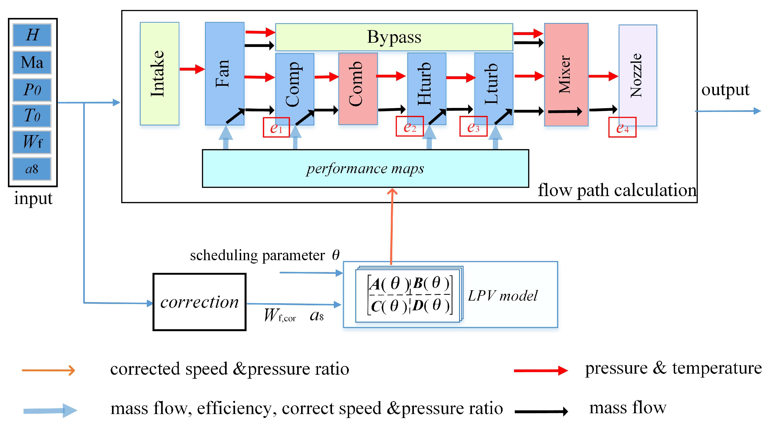
where $\tilde{f}$ is equivalent to f in Equation (7). An LPV model will be obtained if $\tilde{g}$ is substituted for g in Equation (7), and then, the state x and output $v_{\mathrm{final}}$ of this LPV model can be provided for the flow path calculation in NCLM. This LPV model and flow path calculation are combined into an integrated model. Figure 2 shows the computational flow diagram of this integrated model, where the input vector is the same as that of NCLM. The inputs are given to the flow path calculation and is corrected using similarity criteria according to Reference [25]. The corrected inputs $W_{\mathrm{f},\mathrm{cor}}$ and $a_8$, along with the scheduling parameter $\theta =n_{\mathrm{L}}$ measured from the turbofan engine, are furnished to the LPV model. Note that the scheduling parameters of both the LPV model in integrated model and the traditional LPV model are obtained from NCLM in this paper. The state and output of LPV model calculated according to Equation (12) are provided for performance maps to obtain mass flow and efficiency of each rotor component.

As is shown in Figure 2, iterations and balance equations are not involved in the computational flow diagram. The flow path calculation is executed once in one time step no matter how far the current state is away from the equilibrium point; in such case, the real-time performance of this model will be much better than that of NLCM and will be insensitive to the input noises and disturbances while that of NCLM not. In addition, the number of outputs of the integrated model is the same as that of NCLM because the two models share the same flow path calculation. Meanwhile, there are always two states and four outputs of the LPV model required by the integrated model, and therefore, less parameters will be required than the traditional LPV model if more than 4 outputs of the real-time model are required. Moreover, the LPV model in the integrated model is partly linearized from NCLM. The reserved flow path calculation compensates for aerothermodynamic characteristics neglected by the linearization of traditional LPV model and tends to result in more accurate outputs. Therefore, there would be three evident advantages of this integrated model: the real-time performance is (a) insensitive to the input noises and disturbances, (b) faster than NCLM, and (c) more accurate than the traditional LPV model.

It should be noticed that $∥z_k∥<r_{\mathrm{ub}}$ is ensured in NCLM. However, $z_{\mathrm{final}}={\left[e_1,e_2,e_3,e_4\right]}^{\mathrm{T}}$ caused by the modeling errors of the integrated model is out of restriction in the integrated model. If these modeling errors are under control, the differences between the integrated model and NCLM will be quite small. Conversely, the problem arises that, if the LPV model is not accurate, the modeling errors will have side effects on almost all of the outputs of the model.

4. Implementation and Accuracy Improvement

4.1. Linearization

The inputs of the LPV model are environment temperature $T_{\mathrm{s}0}$, pressure $P_{\mathrm{s}0}$, altitude H, mach number $Ma$, fuel flow $W_{\mathrm{f}}$, and area of nozzle throat $a_8$; the states are two rotor speeds $n_{\mathrm{L}}$ and $n_{\mathrm{H}}$; and the outputs are four pressure ratios ${\pi }_{\mathrm{Fan}}$, ${\pi }_{\mathrm{Comp}}$, ${\pi }_{\mathrm{HPT}}$, and ${\pi }_{\mathrm{LPT}}$. In order to obtain the partial derivative, the state of the system is firstly set to a steady mode, and then, $nx$ linearly independent small perturbations of the state are given respectively. In this process, Equation (14) can be obtained according to Equation (9):

$$\begin{array}{c}\hfill \left\{\begin{array}{c}\Delta {\dot{x}}_{\mathrm{p},k}^i=A_{\mathrm{p}}\Delta x_{\mathrm{p},k}^i\\ \Delta y_{\mathrm{p},k}^i=C_{\mathrm{p}}\Delta x_{\mathrm{p},k}^i\end{array}\right.,i=1,2,\cdots nx\end{array}$$

(14)

where $\Delta x_{\mathrm{p},k}^i$ stands for the state derivative at the kth time step under the ith perturbation. Then, the partial derivative terms in Equation (9) can be calculated in the form below:

$$\begin{array}{c}\hfill \left\{\begin{array}{c}{A}_{\mathrm{p},k}=\left[\Delta {\dot{x}}_{\mathrm{p},k}^1,\cdots ,\Delta {\dot{x}}_{\mathrm{p},\mathrm{k}}^{nx}\right]{\left[\Delta x_{\mathrm{p},k}^1,\cdots ,\Delta x_{\mathrm{p},k}^{nx}\right]}^{-1}\\ C_{\mathrm{p},k}=\left[\Delta y_{\mathrm{p},k}^1,\cdots ,\Delta y_{\mathrm{p},k}^{nx}\right]{\left[\Delta x_{\mathrm{p},k}^1,\cdots ,\Delta x_{\mathrm{p},k}^{nx}\right]}^{-1}\end{array}\right.\end{array}$$

(15)

The Equation (15) reveals that $A_{\mathrm{p}}$ and $C_{\mathrm{p}}$ can be calculated at every discrete time k and taht the partial-derivative terms have a very close connection with the dynamic property of the system, and it is obvious that the square matrix $\left[\Delta x_{\mathrm{p},k}^1,\Delta x_{\mathrm{p},k}^2,\cdots ,\Delta x_{\mathrm{p},k}^{nx}\right]$ need to be non-singular. If $\left[\Delta x_{\mathrm{p},k}^1,\Delta x_{\mathrm{p},k}^2,\cdots ,\Delta x_{\mathrm{p},k}^{nx}\right]$ is close to a singular matrix, less upper bounds $r_{\mathrm{ub}}$ of iterations of NCLM are required and the given perturbations should be adjusted or the order of the linear system should simply be reduced.

4.2. Simplification

Equation (11) can be transformed as follows:

$$\begin{array}{c}\hfill \left\{\begin{array}{c}\dot{x}=A_{\mathrm{p}}\left(\theta \right)x+B_{\mathrm{p}}\left(\theta \right)u+M\left(\theta \right)\\ y=C_{\mathrm{p}}\left(\theta \right)x+D_{\mathrm{p}}\left(\theta \right)u+N\left(\theta \right)\end{array}\right.\end{array}$$

(16)

where the equilibrium information is separated into $M\left(\theta \right)=-A_{\mathrm{p}}\left(\theta \right)x_{\mathrm{e}}-B_{\mathrm{p}}\left(\theta \right)u_{\mathrm{e}}$ and $N\left(\theta \right)=y_{\mathrm{e}}-C_{\mathrm{p}}\left(\theta \right)x_{\mathrm{e}}-D_{\mathrm{p}}\left(\theta \right)u_{\mathrm{e}}$. The equilibrium manifold $M\left(\theta \right)$ and $N\left(\theta \right)$ need to be additionally stored. To reduce the number of stored data, $M\left(\theta \right)$ and $N\left(\theta \right)$ are integrated into a typical quasi-LPV structure:

$$\begin{array}{c}\hfill \left\{\begin{array}{c}\dot{x}=A\left(\theta \right)x+B\left(\theta \right)u\\ y=C\left(\theta \right)x+D\left(\theta \right)u\end{array}\right.\end{array}$$

(17)

where $A\left(\theta \right)=A_{\mathrm{p}}\left(\theta \right)+\left[M\left(\theta \right)\begin{array}{cc}/x_1& 0_{nx\times (nx-1)}\end{array}\right]$, $C\left(\theta \right)=C_{\mathrm{p}}\left(\theta \right)+\left[\begin{array}{cc}N\left(\theta \right)/x_1& 0_{nx\times (nx-1)}\end{array}\right]$, $B\left(\theta \right)=B_{\mathrm{p}}\left(\theta \right)$, $D\left(\theta \right)=D_{\mathrm{p}}\left(\theta \right)$, $\theta =x_1$. It is assumed that the current state x and input u are approximately close to a nearby equilibrium point $(u_{\mathrm{e}},x_{\mathrm{e}})$, where $x_{\mathrm{e},1}\approx x_1$, $u\approx u_{\mathrm{e}}$, and the scheduling parameter $\theta$ can be obtained from the current state. The relationship between the coefficients and the scheduling parameter $\theta$ can be seen as a scalar function; thus, the number of the required parameters can be reduced by fitting curves:

$$\begin{array}{c}\hfill q\left(\theta \right)=\sum _{i=0}^m{q}_i{\theta }^i,i=1,2,\dots ,m\end{array}$$

(18)

where $q\left(\theta \right)$ stands for the element of the matrices in Equation (17), $q_i$ is the polynomial coefficients similar to that of Reference [19], and m is the selected order of the polynomial formula.

4.3. Accuracy Improvement

Figure 3 shows the state response from an initial state of $\Delta n_{\mathrm{H}}=0.02$ and $\Delta n_{\mathrm{L}}=0$ at the design point (H = 0, $Ma$ = 0, $W_{\mathrm{f}}$ = 1, $a_8$ = 1). As is shown in the Figure 3a, the low-pressure and high-pressure speeds decrease to zero quickly. In Figure 3b, the logarithm is used to make the variation in the state derivative more easily observed, the magnitude of $\left[\Delta x_{\mathrm{p},k}^1,\Delta x_{\mathrm{p},k}^2,\cdots ,\Delta x_{\mathrm{p},k}^{nx}\right]$ comes to ${10}^{-5}$ within 1.6 s, and the truncation error of the state derivative will play a role in the calculation of $A_{\mathrm{p},k}$. Meanwhile, the sharp decline in Figure 3b indicates that the state derivative fluctuates up and down around 0 due to the drawback of the discrete computation of the energy balance equations in Equation (5). Therefore, there will be imaginary parts in the eigenvalues of $A_{\mathrm{p},k}$.

Figure 3. State response under a disturbance $\Delta n_{\mathrm{H}}=0.02$. (a) conventional coordinate; (b) logarithmic coordinate.

The truncation error is caused by the discrete calculation of the NCLM. The numerical iteration becomes convergent with a convergence upper bound residual $r_{\mathrm{ub}}$ in Equation (6). Figure 4 shows that the convergent value is related to the initial state. If the initial states $x_0^{\prime },x_0^{″}$ of the system are different and $r_{\mathrm{ub}}=r_1$, the iterative solutions $x_{r1}^{\prime }$ and $x_{r1}^{″}$ will be different. It is obvious that a smaller upper bound $r_{\mathrm{ub}}=r_2<r_1$ makes the steady states closer to the real solution $x_{\mathrm{e}}$ in the center and the distance between the steady states smaller: $\left|\right|x_{r2}^{\prime }-x_{r2}^{″}\left|\right|<\left|\right|x_{r1}^{\prime }-x_{r1}^{″}\left|\right|$. Therefore, a smaller $r_{\mathrm{ub}}$ makes the calculation of $\Delta x=x-x_{\mathrm{e}}$ more credible when different perturbations are imposed on the NCLM and, therefore, reduces the influence of the truncation error.

Figure 4. Relationship between the equilibrium states and the convergence residual.

Figure 5a shows the elements of $A_k$ in different times k at the design point with $r_{\mathrm{ub}}={10}^{-4}$. It indicates that, as the truncation error of the NCLM increases, the elements of $A_k$ tend to diverge. Figure 5b shows that a smaller convergence residual $r_{\mathrm{ub}}={10}^{-8}$ can make the elements vary slowly. A can be obtained by the following:

$$\begin{array}{c}\hfill A=1/N_A\sum _{k=1}^{N_A}{A}_k\end{array}$$

(19)

where $N_A$ denotes the number of the selected $A_k$.

Figure 5. Distribution of the elements of $A_k$. (a) $r_{ub}={10}^{-4}$. (b) $r_{ub}={10}^{-8}$.

The NCLM adopts a lot of piecewise linear interpolations to simplify the computation, such as the performance maps mentioned in Section 2. It leads to discontinuous steady and dynamic property of the NCLM and discontinuous elements of the matrices in LTI. In Figure 6a,c, the inputs are $H=0$, $Ma=0$, $a_8=1$, $\mathrm{s}0=101.325$ kPa, and $T_{\mathrm{s}0}=288.15$ K and the fuel flow is given from 0.2 to 1.05 at an interval of 0.01. Eighty-five LTI models are established around these points, and the number of required parameters is 1700. With simplification and 3-order polynomial curve fitting, only 150 parameters is required. The figures show that $dh/du$ and the elements of A are piecewise when $n_{\mathrm{L},\mathrm{e}}=0.7,0.8,0.85,0.9,0.95,1$ and that the values of $n_{\mathrm{L},\mathrm{e}}$ are the exact boundaries of the piecewise interpolation function in the calculation of the performance maps of the fan and the compressor. In order to obtain continuous parameters of the indexed collection of LTI models, the linear interpolation used in the performance maps is replaced by a 3-order spline-fit interpolation, and the elements and the eigenvalues of A become obviously continuous in Figure 6b,d. This differentiable interpolation can improve the dynamic tracking performance of the LTI model. Figure 7 shows the comparison of the state responses of the system, and $n_{\mathrm{L}}$ works across a boundary of the piecewise interpolation function of performance maps, where the initial states are $n_{\mathrm{L}}=0.91$ and $n_{\mathrm{H}}=0.96$; the inputs are $H=0$, $Ma=0$, $W_{\mathrm{f}}=0.73$, and $a_8=1$; and the final states are $n_{\mathrm{L}}=0.89$ and $n_{\mathrm{H}}=0.948$. The response of $n_{\mathrm{L}}$ of spline interpolation is apparently better than that of linear interpolation.

Figure 6. The continuity of $dh/du$ and the elements of A: (a) Linear interpolation, (b) spline interpolation, (c) linear interpolation, and (d) spline interpolation.

Figure 7. The comparison of state response of linear systems: (a) Response of $n_{\mathrm{L}}$; (b) response of $n_{\mathrm{H}}$.

It should be noticed that the spline interpolation is adopted in NCLM to make the parameters of LPV model continuous to improve accuracy around the boundary of former piecewise interpolation in NCLM. The former NCLM adopting linear interpolation is established based on test data and can be seen as a “precise” model, and the NCLMs mentioned elsewhere all stand for this “precise” model.

5. Simulation Results

In this section, the accuracy and computational complexity of the integrated model will be discussed. Comparisons among the integrated mechanism model, the NCLM, and the traditional LPV model are also carried out. The outputs of these models are $P_3,P_4,P_{43},P_6,T_3,T_4,T_{43},T_6$, and F. All the simulation experiments are conducted on a personal computer with an Intel Core i7-6500U CPU and 8 GB Memory.

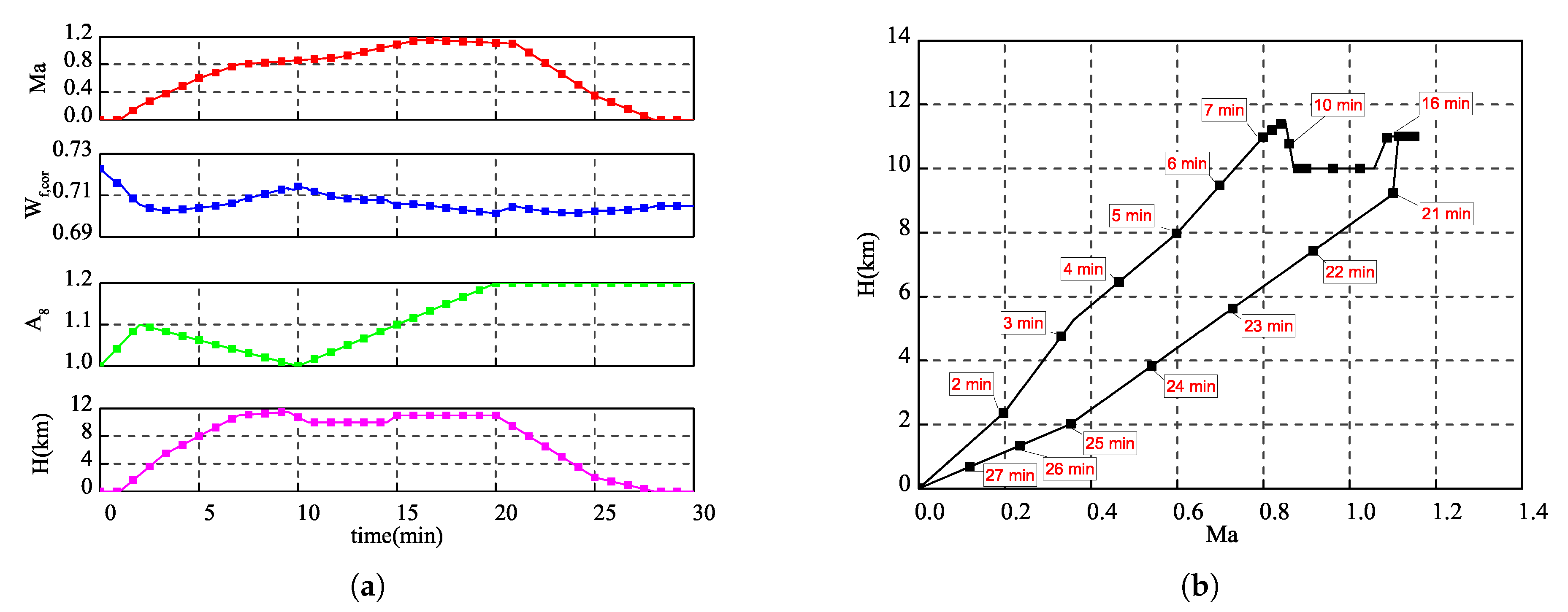
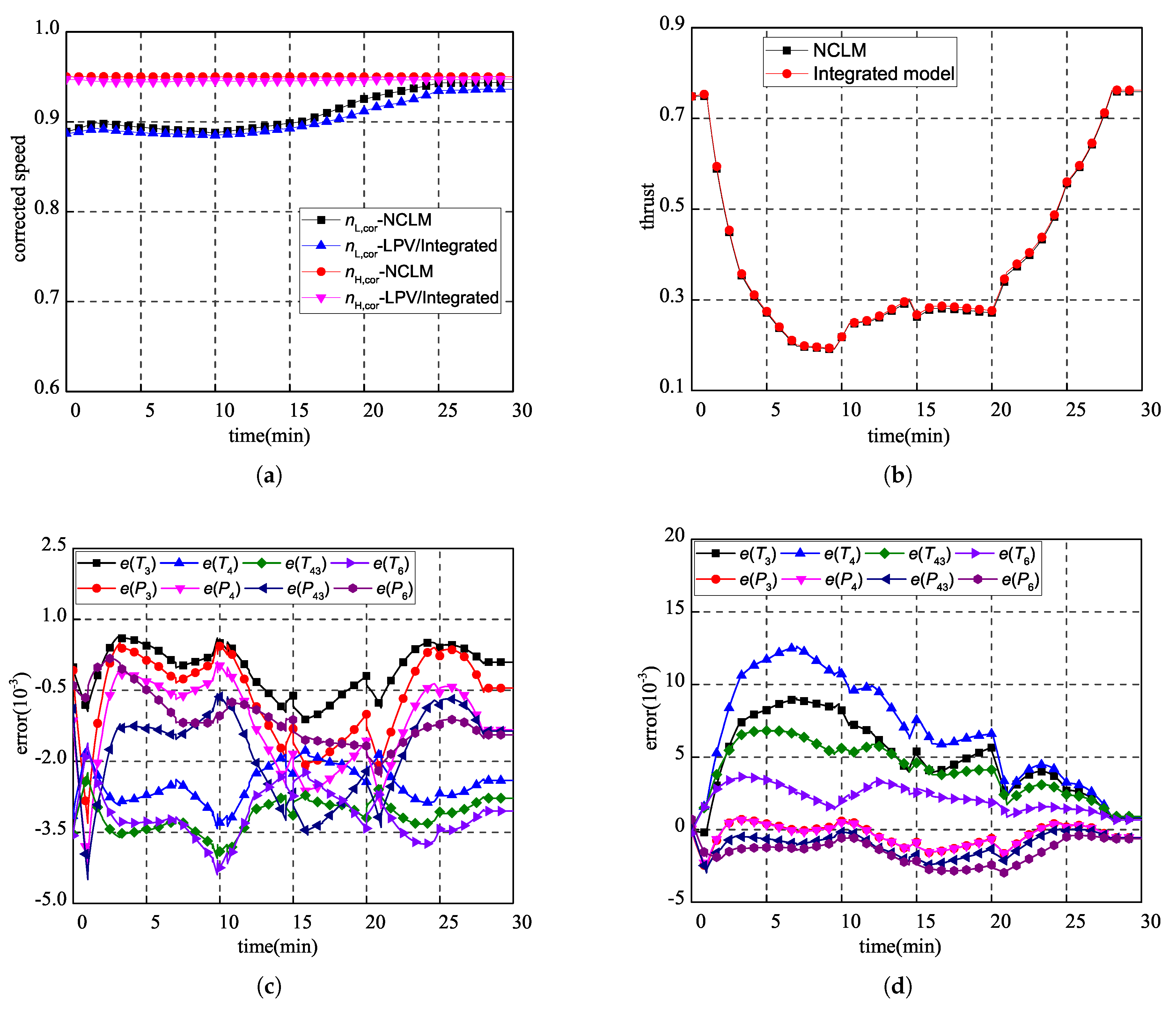
The inputs are given in Figure 8a,b, and the states and outputs are shown in Figure 9. The integrated model and the traditional LPV model share the same states and matrices A and B according to Equation (17), and thus, the responses of the states are the same in Figure 9a. Compared with the maximum absolute error (MAE) of the NCLM, the MAE of the states ($n_{\mathrm{L}}$ and $n_{\mathrm{H}}$) is less than 1.32% and the root mean square error (RMSE) is 0.77% in Table 1. The MAE of the outputs of the integrated model is 0.45%, which is less than that of the traditional model. In Table 1, the bold data shows that the integrated model significantly improves the accuracy of $T_3,T_4,T_{43},P_6$ and, therefore, improves the average MAE and RMSE.

Figure 8. The inputs of the simulation: (a) 4 inputs without noise and (b) flight envelope.

Figure 9. Comparison between the nonlinear component level model (NCLM) and the integrated model: (a) Comparison of state, (b) comparison of thrust, (c) output error of the integrated model, and (d) output error of the traditional linear parameter varying (LPV) model.

Table 1. maximum absolute error (MAE) and root mean square error (RMSE) (%).

	${\mathit{n}}_{\mathbf{L}}$	${\mathit{n}}_{\mathbf{H}}$	${\mathit{T}}_3$	${\mathit{P}}_3$	${\mathit{T}}_4$	${\mathit{P}}_4$	${\mathit{T}}_{43}$	${\mathit{P}}_{43}$	${\mathit{T}}_6$	${\mathit{P}}_6$	F	Average
MAE-Integrated	1.32	0.55	0.12	0.33	0.34	0.43	0.41	0.45	0.44	0.23	0.64	0.48
MAE-Traditional	1.32	0.55	0.90	0.29	1.27	0.27	0.68	0.30	0.37	0.31	_	0.63
RMSE-Integrated	0.77	0.41	0.05	0.11	0.25	0.15	0.32	0.21	0.32	0.12	0.40	0.28
RMSE-Traditional	0.77	0.41	0.55	0.08	0.76	0.08	0.45	0.13	0.23	0.17	_	0.36

In fact, the inputs inevitably contain noises caused by sensors or disturbances, and therefore, perturbations on the inputs should be considered when verifying the accuracy and real-time performance of the considered models. A normally distributed pseudorandom noise $\omega \sim N(0,{0.004}^2)$ is added to the fuel flow in Figure 8a while the other three inputs remain the same. Table 2 shows the time consumption of each model over a thirty-minute simulation. $t_{\mathrm{c}1}$ and $N_{\mathrm{flowpath}1}$ stand for the time consumption and the number of flow path calculations, respectively, with smooth inputs, while $t_{\mathrm{c}2}$ and $N_{\mathrm{flowpath}2}$ stand for the time consumption and the number of flow path calculations taking account of input noises, respectively.

Table 2. Comparison of time consumption and iterative number.

	${\mathit{t}}_{\mathbf{c}1}$ (s)	${\mathit{N}}_{\mathbf{flowpath}1}$ ($\times {10}^4$)	${\mathit{t}}_{\mathbf{c}2}$ (s)	${\mathit{N}}_{\mathbf{flowpath}2}$ ($\times {10}^4$)
NCLM	32.54	45	65.43	104
Integrated model	7.32	9	7.25	9
Traditional LPV model	1.95	0	1.94	0

It can be concluded that the time consumption mainly depends on the number of flow path calculations. Therefore, when the input noise is considered, the time consumption and the number of flow path calculations of the NCLM increase evidently, while those of the integrated model and traditional LPV model are almost not affected. In Table 3, the noise has a slight side effect on the accuracy of all the outputs of the two models. The bold data shows that, similar to Table 2, the integrated model can also improve the accuracy of $T_3,T_4,T_{43}$, and $P_6$ and the average MAE and RMSE when the noises are considered.

Table 3. MAE and RMSE considering the input noise (%).

	${\mathit{n}}_{\mathbf{L}}$	${\mathit{n}}_{\mathbf{H}}$	${\mathit{T}}_3$	${\mathit{P}}_3$	${\mathit{T}}_4$	${\mathit{P}}_4$	${\mathit{T}}_{43}$	${\mathit{P}}_{43}$	${\mathit{T}}_6$	${\mathit{P}}_6$	F	Average
MAE-Integrated	1.40	0.61	0.20	0.43	0.44	0.53	0.49	0.55	0.52	0.30	0.76	0.57
MAE-Traditional	1.40	0.61	0.97	0.38	1.43	0.37	0.81	0.40	0.49	0.38	_	0.72
RMSE-Integrated	0.77	0.41	0.06	0.12	0.25	0.16	0.32	0.21	0.32	0.13	0.41	0.29
RMSE-Traditional	0.77	0.41	0.55	0.10	0.76	0.10	0.45	0.14	0.23	0.18	_	0.37

6. Conclusions

In order to obtain a mechanism model of turbofan engine with satisfactory real-time performance and accuracy, an integrated model is proposed. The iteration in NCLM is substituted by an LPV model to improve the real-time performance, and the flow-path calculation is integrated with the LPV model to preserve the nonlinearity and aerothermodynamics of the model. The influence of the residual and the continuity of the NCLM are discussed to improve the accuracy of the integrated model, and it can be concluded that lower residual and spline-fit interpolation of NCLM make the integrated model more accurate. Simplification and curve fitting are used to reduce the number of the restored parameters. In the simulation, only 8% parameters are required after the simplification.

From the simulation results, the following can be concluded: (a) Compared to NCLM, the proposed model saves over 75% of simulation time if the input noises are not considered and 89% in the presence of the input noises, which means that the real-time performance of the proposed model is insensitive to input noises. (b) When the input noise is neglected, although the integrated mechanism model works slower, it gives better MAE and RMSE values for $T_3$, $T_4$, and $T_{43}$ than the traditional LPV model. Meanwhile, the average MAE and RMSE of the proposed model decrease by 0.15% and 0.08%, respectively. (c) The real-time performance of the proposed model is insensitive to the input noises, and therefore, the simulation time is nearly the same as the simulation time when ignoring noises. Although the input noises will slightly deprave the accuracy of the two models, the average MAE and RMSE of the proposed model decrease by 0.15% and 0.12%, respectively.

Due to the positive effect of the verification, further researches are encouraged: (a) The proposed model could be applied to other aeroengines that require iteration of balance equation, such as turbojet engine and turboshaft engine, and (b) the accuracy and real-time performance could be verified on hardware in loop.

References

- Szuch, J. Advancements in real-time engine simulation technology. In Proceedings of the 18th Joint Propulsion Conference, Cleveland, OH, USA, 21–23 June 1982; p. 1075. [Google Scholar]
- Lu, J.; Lu, F.; Huang, J. Performance Estimation and Fault Diagnosis Based on Levenberg–Marquardt Algorithm for a Turbofan Engine. Energies 2018, 11, 181. [Google Scholar]
- Kim, Y.; Kim, M.; Oh, S.; Shin, W.; Cho, S.; Song, H.H. A New Physics-Based Modeling Approach for a 0D Turbulence Model to Reflect the Intake Port and Chamber Geometries and the Corresponding Flow Structures in High-Tumble Spark-Ignition Engines. Energies 2019, 12, 1898. [Google Scholar] [CrossRef]
- Jaw, L.C.; Mattingly, J.D. Aircraft Engine Controls Design, System Analysis and Health Monitoring; American Institute of Aeronautics and Astronautics Inc.: Reston, VA, USA, 2009. [Google Scholar]
- Szuch, J.R.; Seldner, K. Real-Time Simulation of F100-PW-100 Turbofan Engine Using the Hybrid Computer; NASA: Washington, DC, USA, 1975.
- French, M.W. Development of a Compact Real-Time Turbofan Engine Dynamic Simulation; Technical Report; SAE Technical Paper; SAE: Warrendale, PA, USA, 1982. [Google Scholar]
- Li, S.l.; Sun, J.G. Application of genetic algorithm to solving nonlinear model of aeroengines. Chin. J. Aeronaut. 2003, 16, 69–72. [Google Scholar] [CrossRef]
- Cai, K.; Xie, S.; Zhang, K. Neural Network Model Research of Some Turbofan Engine Based on Recorded Flight Data. In Proceedings of the 2006 6th World Congress on Intelligent Control and Automation, Dalian, China, 21–23 June 2006; Volume 1, pp. 1857–1860. [Google Scholar]
- Chati, Y.S.; Balakrishnan, H. Aircraft engine performance study using flight data recorder archives. In Proceedings of the 2013 Aviation Technology, Integration, and Operations Conference, Los Angeles, CA, USA, 12–14 August 2013; p. 4414. [Google Scholar]
- Bachnas, A.; Tóth, R.; Ludlage, J.; Mesbah, A. A review on data-driven linear parameter-varying modeling approaches: A high-purity distillation column case study. J. Process. Control 2014, 24, 272–285. [Google Scholar] [CrossRef]
- Pan, M.; Wang, H.; Huang, J. T–S Fuzzy Modeling for Aircraft Engines: The Clustering and Identification Approach. Energies 2019, 12, 3284. [Google Scholar] [CrossRef]
- Montazeri-Gh, M.; Nasiri, M.; Jafari, S. Real-time multi-rate HIL simulation platform for evaluation of a jet engine fuel controller. Simul. Model. Pract. Theory 2011, 19, 996–1006. [Google Scholar] [CrossRef]
- Shamma, J.S. Analysis and Design of Gain Scheduled Control Systems. Ph.D. Thesis, Massachusetts Institute of Technology, Cambridge, MA, USA, 1988. [Google Scholar]
- Alkhoury, Z.; Petreczky, M.; Mercere, G. Identifiability of affine linear parameter-varying models. Automatica 2017, 80, 62–74. [Google Scholar] [CrossRef]
- Turk, D.; Gillis, J.; Pipeleers, G.; Swevers, J. Identification of linear parameter-varying systems: A reweighted l2, 1-norm regularization approach. Mech. Syst. Signal Process. 2018, 100, 729–742. [Google Scholar] [CrossRef]
- Rizvi, S.Z.; Velni, J.M.; Abbasi, F.; Tóth, R.; Meskin, N. State-space LPV model identification using kernelized machine learning. Automatica 2018, 88, 38–47. [Google Scholar] [CrossRef]
- Lu, F.; Qian, J.; Huang, J.; Qiu, X. In-flight adaptive modeling using polynomial LPV approach for turbofan engine dynamic behavior. Aerosp. Sci. Technol. 2017, 64, 223–236. [Google Scholar] [CrossRef]
- Balas, G.J. Linear, parameter-varying control and its application to a turbofan engine. Int. J. Robust Nonlinear Control IFAC Affil. J. 2002, 12, 763–796. [Google Scholar] [CrossRef]
- Gilbert, W.; Henrion, D.; Bernussou, J.; Boyer, D. Polynomial LPV synthesis applied to turbofan engines. Control Eng. Pract. 2010, 18, 1077–1083. [Google Scholar] [CrossRef]
- Bruzelius, F.; Breitholtz, C.; Pettersson, S. LPV-based gain scheduling technique applied to a turbo fan engine model. In Proceedings of the International Conference on Control Applications, Glasgow, UK, 18–20 September 2002; Volume 2, pp. 713–718. [Google Scholar]
- Reberga, L.; Henrion, D.; Bernussou, J.; Vary, F. LPV modeling of a turbofan engine. IFAC Proc. Vol. 2005, 38, 526–531. [Google Scholar] [CrossRef]
- Chung, G.Y.; Prasad, J.; Dhingra, M.; Meisner, R. Real time analytical linearization of turbofan engine model. J. Eng. Gas Turbines Power 2014, 136, 011201. [Google Scholar] [CrossRef]
- Tang, L.; Huang, J.; Pan, M. Switching LPV Control with Double-Layer LPV Model for aeroengines. Int. J. Turbo Jet-Engines 2017, 34, 313–320. [Google Scholar]
- Sun, J. Advanced Multivariable Control Systems of Aeroengines; Beijing Hang Kong Hang Tian Da Xue Chu Ban She: Beijing, China, 2005. [Google Scholar]
- Sugiyama, N. Derivation of system matrices from nonlinear dynamic simulation of jet engines. J. Guid. Control Dyn. 1994, 17, 1320–1326. [Google Scholar] [CrossRef]
© 2019 by the authors. Licensee MDPI, Basel, Switzerland. This article is an open access article distributed under the terms and conditions of the Creative Commons Attribution (CC BY) license (http://creativecommons.org/licenses/by/4.0/).