Abstract
Typically, permanent magnet synchronous machines (PMSMs) with small inductance can achieve a higher power density and higher power factor. Thus, in many industrial applications, more and more PMSMs are being designed with small inductance. Compared with traditional PMSMs, current harmonics in small inductance PMSMs are much more abundant, and the amplitudes are usually high. These current harmonics will cause large eddy current losses (ECLs) on the rotor, making the estimation of ECLs necessary in the design stage. Currently, ECL estimation methods are usually based on frequency order information, which cannot tell the travelling direction of the harmonic magneto-wave, resulting in the inaccuracy of the estimation. This article proposes a novel estimation method based on the mechanism of the formation of space-vector pulse width modulation (PWM), which considers both the frequency order and travelling direction of the harmonic wave, resulting in the improvement of the accuracy. Besides this, by using double Fourier analysis (DFA) instead of traditional fast Fourier analysis (FFA), the predicted frequencies of the current harmonics are more accurate and free of the troubles caused by traditional FFA-based methods. Simulation study and experiments are conducted to show the effectiveness of the proposed method.
1. Introduction
Permanent magnet synchronous machines (PMSMs) with small inductance usually have good performance in terms of their power density, dynamic performance and overload capability; thus, they have been a trend in academia and industry. However, small inductance also introduces many disadvantages, such as large current harmonics, high rotor temperature rises, or noise and vibration problems. One key problem of the rotor eddy current loss attenuation, which relates to the rotor temperature rise, is unique to these types of machine because of the poor heat dissipation environment of the rotor and large current harmonics under voltage-source inverter (VSI) supply. Researchers found that a conductive sleeve over the rotor can reduce the eddy current losses (ECLs) significantly, and a great deal of research has been conducted into the performance of different configurations and structure parameters [1,2,3,4]. Meanwhile, continuous efforts have been devoted to the harmonic suppression algorithm of the currents produced by VSI [5,6,7,8,9]. Moreover, the rotor ECL estimation under different control strategies has become an important step for the lifetime guarantee and safety of the PMSMs when designing small inductance PMSMs.
Regarding the estimation method of rotor ECLs, there are mainly two categories: the finite-element method (FEM) and analytical model method. The first one is highly developed and accurate but is time-consuming and needs extensive computation resources. The latter one is fast and provides much information on the improvement of the inverter-motor system; however, it is less accurate than FEM. Thus, analytical methods are usually used in the design process, and FEMs are used to verify the results.
A large number of researchers have devoted themselves to the improvement of analytical methods, mainly concentrating on analytical motor models. Analytical motor models can be roughly divided into two categories: methods considering the reaction field, and methods without considering the reaction field. The first ones have the ability to take the saturation effect, slot opening effect, etc. into consideration, under the assumption that the eddy current field is of the resistance type. Two-dimensional models were developed with polar coordinates [10,11,12,13] or Cartesian coordinates [14], and the permeability of the stator and rotor cores is supposed to be infinite [15,16]. In [17], the time harmonics are discussed, and an extended model was developed. The slotting effect on the eddy current can be modeled using conformal mapping [18] or subdomain models [19,20], and the saturation effect is usually handled using modulation functions [21,22,23] or magnet equivalent circuits (MEC) [24]. Finite magnet dimensions were solved by adding a coefficient to infinite magnet dimensions in [25,26]. In [27], the authors used Carter’s theory and surface impedance to calculate the ECLs, which is simple and has a low computational burden. When the eddy current field cannot be considered to be of the resistance type, which is the case when the thickness of conductor is thicker than the skin depth, the reaction field has to be considered. In [28], the eddy current reaction field was considered in a slotless PMSM. In [29], a 2D model based on Cartesian coordinate was proposed to calculate the losses in the magnet, while in [30], a 2D model based on polar coordinates was proposed. Generally, methods without consideration of the reaction field are more capable of handling complex structures with low-frequency harmonics, while methods which consider the reaction field are more suitable for simple structures with high-frequency harmonics.
The accuracy achieved by the analytical method depends on two aspects: the degree of conformity of the predicted stator current with the actual stator current, and the degree of conformity of the simplified model with the actual motor structure. This article aims to improve the method by reducing the disconformity induced by mismatched currents. For this aspect, traditional methods use the fast Fourier transform (FFT) to decompose the voltage pulses generated by the inverter and then calculate current harmonics based on the frequency spectrum of voltage pulses. These methods are fast, but under non-integer carrier wave ratios, the spectrum leakage problem deteriorates the accuracy of predicted stator current. With the development of simulation technology, many researchers use simulation software such as Simulink from Mathworks to obtain simulated current waveforms, then decompose current waveforms to obtain the frequency spectrum of the stator current. The usage of simulation software greatly improves the accuracy of the prediction of stator current; however, the process is complex, time-consuming, and reveals fewer insights into the difference between various working conditions.
This article proposes a novel ECL estimation method with improved accuracy for PWM inverters. Based on the mechanism of the formation of PWM waveforms, a new decomposition method of PWM voltage pulses is proposed to avoid the problem of spectrum leakage. With the new decomposition method, the phase sequence of different harmonics can be retrieved, which cannot be done with simple FFT or simulation. Regarding the conversion of voltage spectrum into current spectrum, the effect of different voltage components on the motor is discussed. Finally, based on the information provided by the new decomposition method, the direction of the travelling wave caused by subharmonics is carefully studied, and a new algorithm for the calculation of ECLs with different travelling wave direction judgement methods is given.
As the most widely used PWM strategy, space-vector PWM (SVPWM) is adopted as the study object. An analytical orthogonal model of the air-gap is used to ensure accuracy while keeping the model simple, and phase inductance is assumed to be constant.
2. Problem Statement
A typical structure of a small inductance permanent magnet synchronous machine is shown in Figure 1a. The stator is composed of a stator iron core and stator windings, and the rotor is composed of a retaining sleeve, permanent magnet and rotor yoke.
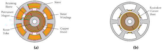
Figure 1.
Structure of small inductance permanent magnet synchronous machine (PMSM) (a) and simplified model for the calculation of eddy current losses (b).
Due to the relatively high permeability in the stator iron core, the windings can be expressed as current sheets at the slot openings. The retaining sleeve is used to enhance the rotor mechanical strength and made of glass fiber. When considering eddy current losses, the retaining sleeve is often considered as part of the air gap because of its low conductivity. The copper shield, which has a high conductivity, is used to reduce the eddy current losses in permanent magnets. Additionally, the simplified model used for eddy current losses estimation is shown in Figure 1b.
Further, the model can be expanded into Cartesian coordinates for convenience in calculation. Typically, a small inductance PMSM Cartesian coordinate model for the calculation of ECLs consists of six layers: the outermost layer is the stator, whose magnet permeability is considered as infinity; next is the current sheet layer, representing the current of the stator, whose thickness is zero; the third layer is the air-gap, whose thickness is d0; then, the copper sleeve used to resist eddy currents, whose thickness is dr; inside the copper sleeve is the permanent magnet layer, whose thickness is dp; and the innermost layer is the rotor yoke, whose thickness is dz. These layers are depicted in Figure 2.
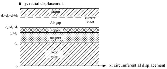
Figure 2.
Model structure of a high-speed PMSM for eddy current loss (ECL) calculation.
To calculate the rotor ECLs, the spectrum of phase voltage of the small inductance PMSM is first calculated using time-FFT, with its base frequency being the fundamental current frequency, and the current harmonics are derived using the amplitudes of voltage harmonics divided by the reactance of each phase; then, the space harmonics caused by the winding structure in the motor are calculated using space-FFT, with its base period being a pole pitch of the motor. This process can be expressed as in Equation (1):
where u(t) is the phase voltage, ωb is the base frequency, n is the order of the current harmonics, Ls is the phase inductance, and In is the amplitude of current harmonics.
Once current harmonics and space harmonics are obtained, their impacts on the motor can be represented by a sum of travelling current sheets. If the order of the current harmonics is n, and the order of space harmonics is v, there would be a travelling current sheet cs(i,x) close to the inner surface of the stator, and that can be expressed as in Equation (2) [19,20]:
where Ksov and Kdpv are coefficients accounting for the slot opening effect and winding distribution effect, respectively. The direction of the travelling current sheet depends on the space harmonic order as well as the current harmonic order. Then, the ECL caused by each current sheet is calculated individually, then summed together to form the overall eddy current loss JLoss. To do so, the vector potential of the motor Az should be calculated. The governing law in the object small inductance PMSM is listed in Equation (3):
where i denotes different layers; e.g., i = 1 denotes the airgap, i = 2 denotes the copper shield, etc. In different layers, σi and μi have different values, depending on the material. For example, in the airgap, σ1 is 0, and μ1 is the permeability of the vacuum. Boundary conditions are given in Equations (4)~(6):
Finally, once the vector potential Az is obtained, Poynting’s Theorem is used to calculate the loss:
where C0 and D0 are related to the specific vector potential of the motor. Detailed calculations are shown in Appendix A.
The problem relates to the way PWM voltage waves are formed: according the results in [30], the PWM modulation process can be seen as a two-variable controlled process. Taking space-vector PWM as an example, the modulation process can be viewed as a line crossing the area formed by a modulating wave, as shown in Figure 3.
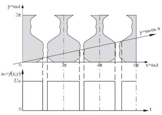
Figure 3.
Graphical representation of space-vector PWM modulation process.
In Figure 3, when the line is in the shaded area, the SVPWM modulator outputs a positive voltage; otherwise, it outputs a negative voltage. The borderline of the shaded area and unshaded area is the shape of the modulation waveform. According to [31], the main frequency components of this process result in multiples of carrier wave frequency and sums of the multiples-of-carrier-wave-frequency and multiples-of-modulation-wave-frequency. The decomposition can be expressed as in Equation (8):
where ω0 is the modulation wave frequency, and ωc is the carrier wave frequency. However, ωc is chosen so that the switching losses of power devices are within a reasonable range and need not be exact multiples of ω0. This made it difficult for all harmonic components to find a common base. If the fundamental current frequency continues to act as the base for time-FFT analysis, spectrum leakage is unavoidable, making the eddy current loss calculation inaccurate. Furthermore, while traditional methods only consider the frequencies of harmonic currents, it will be seen in Section 5 that only one part of the harmonic order pair determines the travelling direction of magneto waves. This error is especially serious in high-speed applications because the modulation wave frequency is relatively high compared to conventional machines. To solve these problems, improved methods for the decomposition of PWM voltage and a novel estimation algorithm to improve the ECL estimation accuracy with different travelling wave direction judgement methods are proposed in this article.
3. SVPWM Working Principle and Expression Deduction of Modulation Wave Per Phase
SVPWM works based on the volt–second balance principle. As depicted in Figure 4, there are six effective vectors and two zero vectors in the stationary plane, and we divide the plane into six sectors. Under SVPWM, the target space vector is synthesized using two neighboring effective vectors and zero vectors.
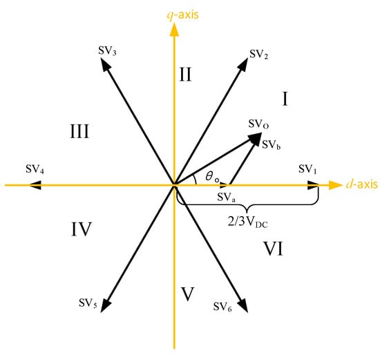
Figure 4.
Synthesis of target space vector under SVPWM modulation.
Suppose the target space vector lies in sector I in Figure 4; the synthesis principle can then be expressed as in Equation (9).
If target space vector is expressed in complex form, as in Equation (10),
then the length of the two effective space vectors of which the target space vector is composed can be derived as in Equation (11):
The action time of two effective vectors can be derived by solving Equation (11), and the result is Equation (12):
Finally, the action times of the effective space vectors in other sectors are derived in a similar way, as listed in Table 1.

Table 1.
Action time of effective space vectors under SVPWM.
The expression of the modulation wave can then be obtained. Taking phase A as example, the expression is listed in Table 2.
Table 2.
Phase A modulation wave expression under SVPWM.
4. Refined SVPWM Frequency Spectrum Structure
Once the expression of the modulation wave is derived, the frequency spectrum structure of the voltage pulses produced by SVPWM can also be derived using double Fourier analysis (DFA). Generally, the pulses produced by SVPWM can be decomposed into a series of sine wave bands, namely the base band, carrier wave bands and sideband harmonics. This can be expressed as in Equation (13):
The coefficients can be obtained using Table 2, shown as Equation (14):
Suppose the modulation ratio M = Uo/VDC; then, the integral limits of the coefficients are listed as shown in Table 3.
Table 3.
Integral limits for modulation wave per phase under SVPWM.
Through cumbersome simplification, the analytical solution of the voltage harmonics is shown in Equation (15):
where
in which Jn denotes the n-th order Bessel function.
It can be noticed that, in Equation (16), Bmn = 0. This implies that the ideal modulation process does not change the phase of the modulation wave. Furthermore, when m ≥ 1, n ≠ 3k, Amn does not have to be zero; however, when m = 0, n ≠ 3k, Amn does have to be zero. This implies that an ideal modulation process does introduce new frequency components into the modulated voltage waveform.
For phase B and C, the expressions are shown as in Equations (17) and (18),
where the coefficient Amn+jBmn is the same as phase A.
When calculating harmonic currents, the amplitude of current can be calculated using Equation (19):
however, the respective phase of voltage harmonics must be considered. From Equations (17) and (18), the following can be seen:
- When n = 3k, the coefficients in fa(t), fb(t) and fc(t) are the same. Thus, the harmonic voltage does not produce a respective resulting harmonic current.
- Switching harmonics does not exist in phase currents; i.e., the voltage harmonics bearing the form in Equation (20)do not produce current harmonics. This is because the coefficients of such voltage harmonics are the same in all three phases.
- Voltage harmonics with m ± n being even do not produce current harmonics either. The reasons for this are as follows.Components bearing the form in Equation (21)will not produce current harmonics because =0.Components bearing the form in Equation (22)will not produce current harmonics because = 0 when m and n are both even or odd, which is a synonym of m ± n being even.Components bearing the form in Equation (23)will not produce current harmonics because = 0 when m and n are both even or odd, which is another synonym of m ± n being even.Components bearing the form in Equation (24)will not produce current harmonics; the reason for this is similar.
5. ECL Estimation Algorithm with Different Travelling Current Sheet Direction Judgement Methods
The travelling direction of current sheets partly depends on the space harmonics and partly on current harmonics. For simplicity, we suppose that space harmonics are only caused by a non-sinusoidal property of stator winding. Other sources of space harmonics, including non-constant permeability, are neglected.
We take a two-pole, 12-slot permanent magnet synchronous machine as the study object. The cross-section of this machine is shown in Figure 5.

Figure 5.
Structure of target permanent magnet synchronous machine.
The winding structure of phase A can be expressed as in Figure 6.
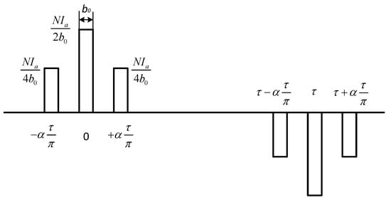
Figure 6.
Winding structure of phase A.
In Figure 6,
α denotes the electrical angle between adjacent slot opening;
N denotes the winding turns of a single phase;
b0 denotes the width of one slot opening;
τ denotes the pole pitch; and
Ia denotes the current in a phase winding.
Thus, the current sheet of phase A can be expressed as in Equation (25):
Similarly, the current sheet expressions of phase B and phase C are listed in Equations (26) and (27):
As mentioned in Section 4, the current waveforms can be expressed as in Equation (19). Then, the overall travelling current sheet can be derived by adding three current sheets:
where
It can be seen that only the current harmonic order n has an influence on the direction of the travelling wave, while current harmonic order m has nothing to do with the travelling wave direction. Further, this can be divided into two situations:
- (v+n) can be divided by three, while (v-n) cannot:In this situation, the travelling wave travels backwards with regard to the rotor. Suppose the velocity of the outer rotor of the permanent magnet synchronous machine is vr; then, the travel velocity vtr of the travelling current sheet is expressed as in Equation (31):
- (v-n) can be divided by three, while (v+n) cannot:
In this situation, the travelling wave travels forwards with regard to the rotor. Suppose the velocity of the outer rotor of the synchronous machine is vr; then, the travel velocity vtr of the travelling current sheet is expressed as in Equation (33):
Finally, a novel ECL estimation algorithm can be developed. The key steps are shown in Figure 7.
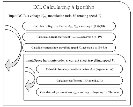
Figure 7.
Novel ECL calculation algorithm.
6. Simulation Study and Experiments
A 2 kW surface-mounted permanent magnet synchronous machine is studied. Its main characteristics are listed in Table 4:
Table 4.
Main parameters for the object PMSM.
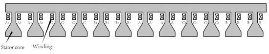
Figure 8.
Winding structure of the object small inductance PMSM.
Table 5.
Structure parameters for the object PMSM.
To highlight the performance of the proposed algorithm, the switching frequency of the inverter is chosen at 10 kHz, which is relatively low compared with the phase inductance and harmonic currents, which would be large as a consequence. Firstly, the voltage and current spectrum prediction methods are verified using a current probe and an oscilloscope. Secondly, the conventional method for calculating the ECLs is conducted against the newly proposed method. Because experimental verification of ECLs is subject to heat conduction, we are unable to separate the mechanic friction loss and other interferences, making it very hard to be accurate; thus, both methods are verified by comparison with FEM results. The FEM software chosen is Flux 2D from Altair, which is widely used in the motor design industry.
The experimental platform is shown in Figure 9.
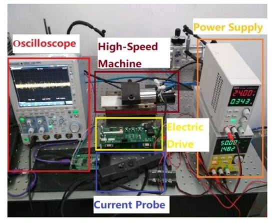
Figure 9.
Experimental platform for the verification of current spectrum prediction.
The electric drive is set to the sensorless vector control work mode. To verify the performance of the proposed method under integer carrier wave ratios and non-integer carrier wave ratios, the base current frequency is chosen at 200 Hz and 240 Hz, with a carrier wave ratio of 50 and 46.667, respectively. Under the SVPWM method, the phase voltage spectrum is shown in Figure 10, and the predicted current distribution is shown in Figure 11.
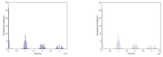
Figure 10.
Phase voltage spectrum at a base frequency of 200 Hz (left) and 240 Hz (right) under SVPWM modulation. The DC bus voltage is 30 V.
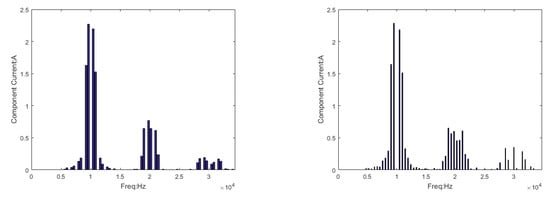
Figure 11.
Phase harmonic current prediction of 200 Hz (left) and 240 Hz (right) under SVPWM modulation. The DC bus voltage is 30 V and the phase inductance is 48 μH.
It can be seen in Figure 11 that, when the base current frequency changed from 200 Hz to 240 Hz, the diversity of the current frequency components and their amplitudes increased greatly. The experimental results are shown in Figure 12.
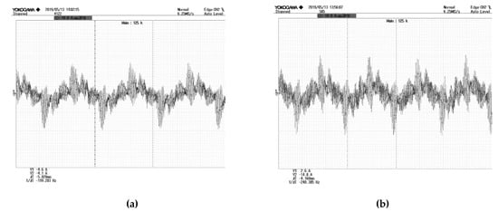
Figure 12.
Experimental current waveform under sensorless vector control mode. The base current frequency is 200 Hz in (a) and 240 Hz in (b).
To make a comparison of the predictive performance of the newly proposed method (DFA) and traditional analysis method (FFT), analyses by both methods are given in Figure 13. Nevertheless, a spectrum analysis of the experimental current waveform is also performed and used as the standard of performance.
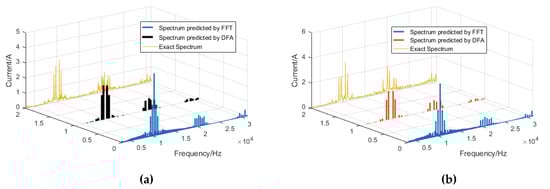
Figure 13.
Performance comparison of current spectrum prediction by newly proposed method (double Fourier analysis (DFA)) and traditional fast Fourier transform (FFT). The base current frequency is 200 Hz in (a) and 24 0Hz in (b). The experimental current spectrum served as the standard.
From Figure 13, it can be seen that traditional methods using FFT decomposition results cannot tell the phase differences among different harmonic components. Thus, traditional methods mispredict some frequency components that do not exist under real conditions. The method proposed in this article, however, fits the experimental results well, proving the effectiveness of the novel method.
The impact of different travelling directions of travelling current sheets on the prediction accuracy of ECLs are verified using FEM software. Firstly, the traditional method based on FFT and the method based on simulation which consider the travelling direction as relative to harmonic frequency are conducted. Then, the method proposed in this article, which uses different travelling direction judgement methods, is conducted, and finally all methods are compared to the results of the FEM software with experimental current waveforms. The results are shown in Figure 14 and Figure 15.
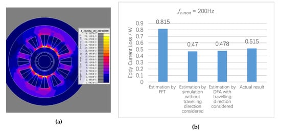
Figure 14.
Eddy current losses estimated with different methods. The base current frequency is 200 Hz. The FEM software calculation is shown in (a), and data are listed in (b).
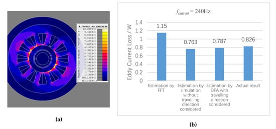
Figure 15.
Eddy current losses estimated with different methods. The base current frequency is 240 Hz. The FEM software calculation is shown in (a), and data are listed in (b).
From Figure 14 and Figure 15, it can be seen that calculation methods based on FFT usually get larger results than reality, while methods based on simulation and DFA obtain results close to the actual result. However, with different travelling direction judgement methods, the ECL estimation scheme proposed in this article showed better accuracy, with improvements up to 1.9%, which proved its effectiveness.
7. Conclusions
In this article, a novel rotor ECL estimation method with improved accuracy for small inductance permanent magnet synchronous machines under SVPWM supply is proposed. A double Fourier analysis-based SVPWM harmonics decomposition algorithm is proposed to replace traditional FFT-based or simulation-based methods, which enables the phase sequence detection of current harmonics. Based on this extra information, a new method of magneto-wave travelling direction judgement is proposed. Regarding the transformation of voltage harmonics to current harmonics, an elimination method by the analysis of the coefficients of different harmonic current components make the misprediction phenomenon disappear compared to FFT-based methods. Finally, these amendments are applied to the 2D analytical motor model, and simulations and experiments showed that the proposed algorithm achieved better accuracy compared with traditional estimation methods after these modifications.
Author Contributions
Conceptualization, L.P. and Q.G.; methodology, L.P.; software, L.P.; validation, R.Y., P.D. and Q.G.; formal analysis, L.P.; investigation, L.L.; resources, L.L.; writing—original draft preparation, L.P.; writing—review and editing, L.L.
Funding
This research was funded by the National Natural Science Foundation of China, grant No. 51577038.
Conflicts of Interest
The authors declare no conflict of interest.
Appendix A. Details of the Analytical Model for the Eddy Current Loss Estimation
Due to the small slot opening, the magnet field strength can be viewed as parallel to the stator inner surface. Thus, the windings can be modeled as current sheets at slot openings. The current sheet of phase A can be expressed as in Equation (A1):
Similarly, the current sheet of phase B and phase C can be expressed as in Equations (A2) and (A3):
where b0 is the slot opening width, τ is the pole pitch, and α is the winding distribution angle.
Time harmonics in phase currents can be decomposed as in Equation (A4):
We define , , and the total travelling wave current sheet can be expressed as in Equation (A5):
The travelling direction can be determined using the law depicted in Equation (A6):
(v+n) can be divided by three, while (v-n) cannot: current sheet travels forwards:
(v-n) can be divided by three, while (v+n) cannot: current sheet travels backwards:
Now, consider the domaining physical rules in the motor. Since the rotor yoke is laminated, the conductivity is relatively small. For convenience, the conductivity of rotor yoke is reduced to zero. By assuming the vector potential Az = 0 at the rotor shaft, the following can be obtained:
The boundary conditions can be expressed as in Equation (A9):
A solution can be found by assuming , which carries the form in Equation (A10):
where . The subscript i denotes different parts of the motor; e.g., i = 1 when in an air-gap, i = 2 when in the copper sleeve, etc. The whole boundary condition group can be expressed as a matrix multiplication Ax = B, where , , and .
After the solution of Az is found, the eddy current loss of the rotor JLoss is expressed as Equation (A11):
References
- Hannon, B.; Sergeant, P.; Dupré, L. Evaluation of the Rotor Eddy-Current Losses in High-Speed PMSMs With a Shielding Cylinder for Different Stator Sources. IEEE Trans. Magn. 2019, 55, 1–10. [Google Scholar] [CrossRef]
- Riemer, B.; Lebmann, M.; Hameyer, K. Rotor design of a high-speed permanent magnet synchronous machine rating 100,000 rpm at 10 kW. In Proceedings of the 2010 IEEE Energy Conversion Congress and Exposition, Atlanta, GA, USA, 12–16 September 2010; pp. 3978–3985. [Google Scholar]
- Weili, L.; Hongbo, Q.; Xiaochen, Z.; Ran, Y. Influence of copper plating on electromagnetic and temperature fields in a high-speed permanent-magnet generator. IEEE Trans. Magn. 2012, 48, 2247–2253. [Google Scholar] [CrossRef]
- Li, W.; Qiu, H.; Zhang, X.; Cao, J.; Yi, R. Analyses on electromagnetic and temperature fields of superhigh-speed permanent-magnet generator with different sleeve materials. IEEE Trans. Ind. Electron. 2014, 61, 3056–3063. [Google Scholar] [CrossRef]
- Li, L.; Czarkowski, D.; Liu, Y.; Pillay, P. Multilevel space vector PWM technique based on phase-shift harmonic suppression. In Proceedings of the Fifteenth Annual IEEE Applied Power Electronics Conference and Exposition (Cat. No. 00CH37058), New Orleans, LA, USA, 6–10 February 2000; Volume 1, pp. 535–541. [Google Scholar]
- Yu, F.; Zhang, X.; Wang, S. Five-phase permanent magnet synchronous motor vector control based on harmonic eliminating space vector modulation. In Proceedings of the 2005 International Conference on Electrical Machines and Systems, Nanjing, China, 27–29 September 2005; Volume 1, pp. 392–396. [Google Scholar]
- Zhou, C.; Yang, G.; Su, J. PWM strategy with minimum harmonic distortion for dual three-phase permanent-magnet synchronous motor drives operating in the overmodulation region. IEEE Trans. Power Electron. 2015, 31, 1367–1380. [Google Scholar] [CrossRef]
- Li, X.; Chen, G. An Approach to Harmonic Suppression Based on Triple Harmonics Injection with Passive Circuit. Autom. Electr. Power Syst. 2007, 14, 61–65. [Google Scholar]
- Zhang, Y.; Li, Y.W. Investigation and suppression of harmonics interaction in high-power PWM current-source motor drives. IEEE Trans. Power Electron. 2014, 30, 668–679. [Google Scholar] [CrossRef]
- Zhu, Z.Q.; Ng, K.; Schofield, N.; Howe, D. Analytical prediction of rotor eddy current loss in brushless machines equipped with surface-mounted permanent magnets. I. Magnetostatic field model. In Proceedings of the Fifth International Conference on Electrical Machines and Systems, Shenyang, China, 18–20 August 2001; Volume 2, pp. 806–809. [Google Scholar]
- Zhu, Z.Q.; Ng, K.; Schofield, N.; Howe, D. Analytical prediction of rotor eddy current loss in brushless machines equipped with surface-mounted permanent magnets. II. Accounting for eddy current reaction field. In Proceedings of the Fifth International Conference on Electrical Machines and Systems, Shenyang, China, 18–20 August 2001; Volume 2, pp. 810–813. [Google Scholar]
- Fang, D.; Nehl, T.W. Analytical modeling of eddy-current losses caused by pulse-width-modulation switching in permanent-magnet brushless direct-current motors. IEEE Trans. Magn. 1998, 34, 3728–3736. [Google Scholar] [CrossRef]
- Bellara, A.; Bali, H.; Belfkira, R.; Amara, Y.; Barakat, G. Analytical Prediction of Open-Circuit Eddy-Current Loss in Series Double Excitation Synchronous Machines. IEEE Trans. Magn. 2011, 47, 2261–2268. [Google Scholar] [CrossRef]
- Paradkar, M.; Bocker, J. 2D analytical model for estimation of eddy-current loss in the magnets of IPM machines considering the reaction field of the induced eddy currents. In Proceedings of the 2015 IEEE International Electric Machines & Drives Conference (IEMDC), Coeur d’Alene, ID, USA, 10–13 May 2015; pp. 1096–1102. [Google Scholar]
- Atallah, K.; Howe, D.; Mellor, P.; Stone, D. Rotor loss in permanent-magnet brushless AC machines. IEEE Trans. Ind. Appl. 2000, 36, 1612–1618. [Google Scholar]
- Wang, J.; Atallah, K.; Chin, R.; Arshad, W.M.; Lendenmann, H. Rotor Eddy-Current Loss in Permanent-Magnet Brushless AC Machines. IEEE Trans. Magn. 2010, 46, 2701–2707. [Google Scholar] [CrossRef]
- Ishak, D.; Zhu, Z.; Howe, D. Eddy-current loss in the rotor magnets of permanent-magnet brushless machines having a fractional number of slots per pole. IEEE Trans. Magn. 2005, 41, 2462–2469. [Google Scholar] [CrossRef]
- Markovic, M.; Perriard, Y. A simplified determination of the permanent magnet (PM) eddy-current losses due to slotting in a PM rotating motor. In Proceedings of the International Conference on Electrical Machines and Systems (ICEMS), Wuhan, China, 17–20 October 2008; pp. 309–313. [Google Scholar]
- Wu, L.J.; Zhu, Z.Q.; Staton, D.; Popescu, M.; Hawkins, D. Analytical model for predicting magnet loss of surface-mounted permanent magnet machines accounting for slotting effect and load. IEEE Trans. Magn. 2012, 48, 107–117. [Google Scholar] [CrossRef]
- Wu, L.J.; Zhu, Z.Q.; Staton, D.; Popescu, M.; Hawkins, D. Analytical modeling of eddy current loss in retaining sleeve of surface-mounted PM machines accounting for influence of slot opening. In Proceedings of the 2012 IEEE International Symposium on Industrial Electronics, Hangzhou, China, 28–31 May 2012; pp. 611–616. [Google Scholar]
- Rahideh, A.; Korakianitis, T. Analytical magnetic field distribution of slotless brushless permanent magnet motors—Part I. Armature reaction field, inductance and rotor eddy-current loss calculations. IET Electr. Power Appl. 2012, 6, 628. [Google Scholar] [CrossRef]
- Yamazaki, K.; Kanou, Y. Rotor Loss Analysis of Interior Permanent Magnet Motors Using Combination of 2D and 3D Finite Element Method. IEEE Trans. Magn. 2009, 45, 1772–1775. [Google Scholar] [CrossRef]
- Fang, Z.X.; Zhu, Z.Q.; Wu, L.J.; Xia, Z.P. Simple and accurate analytical estimation of slotting effect on magnet loss in fractional-slot surface-mounted PM machines. In Proceedings of the 2012 XXth International Conference on Electrical Machines, Marseille, France, 2–5 September 2012; Volume 37, pp. 464–470. [Google Scholar]
- Jaffar, M.Z.M.; Husain, I. Path permeance based analytical inductance model for IPMSM considering saturation and slot leakage. In Proceedings of the 2017 IEEE International Electric Machines and Drives Conference (IEMDC), Miami, FL, USA, 21–24 May 2017; pp. 1–7. [Google Scholar]
- Wang, J.; Papini, F.; Chin, R.; Arshad, W.M.; Lendenmann, H. Computationally efficient approaches for evaluation of rotor eddy current loss in permanent magnet brushless machines. In Proceedings of the 2009 International Conference on Electrical Machines and Systems, Tokyo, Japan, 15–18 November 2009. [Google Scholar]
- Bode, C.; Canders, W.R. Advanced calculation of eddy-current losses in PMSM with tooth windings. In Proceedings of the XIX International Conference on Electrical Machines, Rome, Italy, 6–8 September 2010; Volume 1, pp. 1–6. [Google Scholar]
- Pyrhonen, J.; Jussila, H.; Alexandrova, Y.; Rafajdus, P.; Nerg, J. Harmonic Loss Calculation in Rotor Surface Permanent Magnets—New Analytic Approach. IEEE Trans. Magn. 2012, 48, 2358–2366. [Google Scholar] [CrossRef]
- Dubas, F.; Rahideh, A. Two-Dimensional Analytical Permanent-Magnet Eddy-Current Loss Calculations in Slotless PMSM Equipped With Surface-Inset Magnets. IEEE Trans. Magn. 2014, 50, 54–73. [Google Scholar] [CrossRef]
- Martin, F.; Zaim, M.E.H.; Tounzi, A.; Bernard, N. Improved Analytical Determination of Eddy Current Losses in Surface Mounted Permanent Magnets of Synchronous Machine. IEEE Trans. Magn. 2014, 50, 1–9. [Google Scholar]
- Arumugam, P.; Hamiti, T.; Gerada, C. Estimation of Eddy Current Loss in Semi-Closed Slot Vertical Conductor Permanent Magnet Synchronous Machines Considering Eddy Current Reaction Effect. IEEE Trans. Magn. 2013, 49, 5326–5335. [Google Scholar] [CrossRef]
- Holmes, D.G.; Lipo, T.A. Pulse Width Modulation for Power Converters: Principles and Practice; John Wiley & Sons: Hoboken, NJ, USA, 2003; pp. 215–257. [Google Scholar]
© 2019 by the authors. Licensee MDPI, Basel, Switzerland. This article is an open access article distributed under the terms and conditions of the Creative Commons Attribution (CC BY) license (http://creativecommons.org/licenses/by/4.0/).