Article

The Effect of Temperature on Flowback Data Analysis in Shale Gas Reservoirs: A Simulation-Based Study

1
School of Energy Resources, China University of Geosciences, Beijing 100083, China
2
Beijing Key Laboratory of Unconventional Natural Gas Geological Evaluation and Development Engineering, Beijing 100083, China
3
Department of Civil and Environmental Engineering, University of Alberta, Edmonton, AB T6G 2W2, Canada
*
Authors to whom correspondence should be addressed.
Energies 2019, 12(19), 3751; https://doi.org/10.3390/en12193751
Submission received: 7 August 2019 / Revised: 19 September 2019 / Accepted: 25 September 2019 / Published: 30 September 2019
(This article belongs to the Section H: Geo-Energy)

Abstract

:
During hydraulic fracturing, there is a temperature difference between the injected water and formation rock for shale gas wells. The objective of this study is to investigate how this temperature difference changes with time, and how it affects multiphase-flow modeling during the shut-in and flowback periods. We conducted numerical simulations to investigate the behaviors of fracture temperature in shale gas wells. The results show a significant increase in fracture temperature during the shut-in and flowback periods. Sensitivity analysis suggests that this temperature increase is strongly related to the thermal conductivity of formation rock, matrix permeability, and initial reservoir temperature. Simulation scenarios were further compared to investigate the effect of temperature on flowback data analysis. Without considering the thermal effect, flowback data analysis may yield an earlier fracture cleanup and overestimated fracture volume. In addition, this study suggests that the thermal effect may also have implications for optimizing flowback operations.

Graphical Abstract

1. Introduction

Hydraulic fracturing is the key technique for economically extracting hydrocarbon from shale reservoirs. During hydraulic fracturing, millions of gallons of water [1] are injected at room temperature into hot shale. As featured by Figure 1, the formation temperature can reach up to 190 °C in shale formations. Studies suggest that the temperature difference between fracturing water and formation rock can affect the failure behaviors of fractures during fracturing treatment [2,3,4,5]. Recently, it has been demonstrated that temperature analysis can qualitatively provide early insights into fracture characterization [6] and fracturing optimization [7,8,9,10]. Bottomhole temperature data were reported to be monitored by distributed sensors behind the wellbore (casing or tubing) during, and shortly after, the fracturing treatment [10,11]. The results show a significant difference between bottomhole temperature and reservoir temperature at the end of fracturing treatment. However, the bottomhole temperature data were measured by sensors at wellbore for a short period, and thus mainly represent the fluid temperature near wellbore. It remains unclear about how temperature is distributed in fractures and far-field reservoir, and how long it takes to warm up the fracturing fluids after the fracturing treatment of shale gas wells.
After the fracturing treatment, shale gas wells often go through a period of shut-in days to prepare production equipment at surface [13,14,15,16,17]. This shut-in period may last from several days to months [16,18,19]. An extended shut-in period of six months has been reported in a gas well completed in Marcellus shale [13]. Recently, several studies [14,20,21,22,23,24] investigated the effect of shut-in days on the production performance of shale gas wells. Numerical simulations were conducted to investigate the environmental aspects of shut-in on the fate of fracturing water [25,26,27,28]. Experimental studies also investigated the water losses during this shut-in period [29,30]. These simulation and experimental studies demonstrated that imbibition plays a key role for the interactions between formation rock and fracturing water during shut-in. As a key drive mechanism of imbibition, capillary force is a function of interfacial tension that further depends on temperature. However, the thermal effect was not considered in most of these studies on the interactions between formation rock and fracturing water during shut-in.
After the fracturing and shut-in periods, shale gas wells go through a process of flowback to return the injected fracturing water before production. Recent studies suggested that the rate and pressure data recorded during flowback can provide a very early opportunity to characterize fracture network after the fracturing treatment [31,32,33]. Several analytical models have been developed to describe the production behaviors during the flowback period [15,34,35,36,37,38]. These studies have demonstrated that applying these models on field flowback data can estimate fracture length, fracture volume, and fracture conductivity. Flowback chemical analysis has also been applied on salinity data to characterize fracture networks [39,40,41,42,43]. In addition, studies have been conducted to investigate the mechanisms of fracture cleanup such as gas vaporizing water [30,44,45]. However, most of the previously-cited flowback studies assumed a constant fluid temperature which reaches the formation temperature as flowback starts, without considering the possible difference between them. Fluid properties such as gas viscosity and formation factor are among the key inputs in flowback analysis; however, fluid properties are also a strong function of temperature. Therefore, it is unclear whether the outputs from flowback analysis will be biased because of the assumption of constant fluid temperature.
In this paper, we present a simulation study to investigate the following questions regarding the temperature behaviors during the shut-in and flowback periods: (1) How long will it take for fluid temperatures to reach the formation temperature? (2) What are the key parameters controlling the changes in fracture temperature? (3) How does fracture-temperature change impact flowback analysis? To answer these questions, we first simulated the fracturing, shut-in and flowback processes using a thermal simulator to obtain the changes in fracture temperature with respect to time and space. We then presented a sensitivity analysis of fracture properties (fracture width and length), reservoir properties (thermal conductivity, reservoir permeability, and initial reservoir temperature), and operational parameter (shut-in days) on the behaviors of fracture temperature. We also compared the results of simulation scenarios with and without considering the thermal effect to show how temperature impacts flowback data analysis. Implications of temperature on field operations are further discussed in the last sections.

2. Model Descriptions

This section describes the base model of reservoir, fracture, and wellbore for simulating the fracturing, shut-in, and flowback processes.

2.1. Reservoir and Fracture Models

In this study, a semi-analytical model (STARS thermal process simulation module, CMG software) was used to simulate the dynamics of temperature in reservoir and fracture during the processes of fracturing, shut-in, and flowback. As illustrated by Figure 2, a 3D gas–water thermal reservoir model was built to simulate the heat transfer and fluid flow during these processes. The section of reservoir volume between two fracturing stages was modeled by a single, planar, bi-wing hydraulic fracture in a vertical wellbore.
Table 1 lists the key reservoir and fracture parameters for the base model. The reservoir and fracture parameters were mainly adopted from previous studies on gas wells completed in the Eagle Ford Shale [46,47,48]. The total dimension of studied region was 400 m × 400 m × 100 m, corresponding to the grid number of 46 × 16 × 20 in X, Y, and Z directions, respectively. Grids near the fractures were refined in a logarithmic distribution to capture the flow at the interface between matrix and fracture. The porosity of the matrix was set to 0.1, and the permeability was set to 0.001 mD. The simulated fracture was located in the center of the simulation domain, perpendicular to the X direction, with a total dimension of 350 m × 55 m × 0.01 m, porosity of 0.6, and permeability of 1000 mD. This study focused on dry-gas wells completed in shale with slickwater as fracturing fluid. As listed in Table 2 and Table 3, we thus adopted the thermodynamic properties of shale rock, dry gas, and water in the simulation.

2.2. Wellbore Model

CMG’s Semi-analytical Wellbore Model (SAM) was used to simulate the two-phase flow in wellbore. Figure 3 shows a schematic of the wellbore model including pipes, cement, and annular spaces. As listed in Table 4, we adopted the commonly-used wellbore parameters in oil industry for the simulation. The equations for the conservation of mass, momentum and heat balance were combined to solve the heat transfer between wellbore and reservoir [55] based on the following assumptions: (a) heat transfer in and around the wellbore takes place under pseudo steady-state conditions, whereas the heat transfer to the formation occurs under unsteady state conditions; (b) the diffusivity and conductivity of the formation are independent of depth and temperature; (c) the tubing hangs symmetrically inside the casing; and (d) the Beggs and Brill two-phase flow correlation [56] is applied to calculate bottomhole pressure.

2.3. Initialization

The simulation was initialized by injecting 2000 m 3 of water into fractures within one day period [48]. The process of injection is followed by a shut-in period of 30 days. After the shut-in period, the temperature behaviors and well performance were simulated for up to 120 days of flowback.

3. Temperature Changes with Time and Space

This section shows the changes in temperature with time and space for the base model. First, it shows the changes in fracture temperature during the processes of fracturing, shut-in, and flowback. Second, it shows the distribution of temperature in the fracture and reservoir.

3.1. The Changes in Temperature with Time

Figure 4 shows the fracture temperature during the periods of fracturing, shut-in and flowback for the base model. The fracture temperature is represented by the average temperature of grid where wellbore centers. Overall, the changes in fracture temperature can be described by the trends of cool-down and warm-up as follows.
Cool-down. During the fracturing period, the fracture temperature decreases from the initial formation temperature of 80 °C to 46 °C. The temperature decrease is close to the field values (around 32 °C) measured by Distributed Temperature Sensing (DST). In addition, the change in fracture temperature is within the range (55–88 °C) reported by previous modeling studies [4,58,59,60,61].
Warm-up. After fracturing treatment, the results show an increasing fracture temperature. As shown in Figure 4, during shut-in periods, the fracture temperature increases from 46 to 73 °C. After fracturing treatment, the results show a significant increase in the early 10 days, and then a general flattening at the late shut-in period. One may expect that during warm-up the temperature increase mainly occurs over the early shut-in period.
After opening the well for flowback, the results show a sudden increase in temperature, and then a gradual increase from 73 to 78 °C. After the shut-in period, the sudden increase in fracture temperature is expected to be caused by the changing mechanism of heat transfer from conduction to convection once flowback starts. By comparing the temperature increase during the shut-in and flowback periods, one may expect that wells with less shut-in days experience a more significant temperature increase in fracture temperature during flowback.
As shown in Figure 4, the wellhead temperature increases in the early 50 days, and then decreases with time during flowback. The increase in wellhead temperature is about 5 °C at early flowback. This increase in wellhead temperature is mainly a response of warm-up process in the reservoir and fracture. The later decreasing wellhead temperature can be attributed to the heat loss into the surroundings of wellbore. The difference between bottomhole and wellhead temperature is around 50 °C. This difference is expected to be caused by the heat loss in the vertical section of wellbore.

3.2. Temperature Distribution

Herein, we show the distribution of temperature in fracture and formation for the base case during the periods of fracturing, shut-in, and flowback.

3.2.1. Temperature Profiles along Fracture

Figure 5 shows the profiles of temperature along the fracture wall during the periods of fracturing, shut-in, and flowback. During the fracturing period, the results show a cool-down process, which is described by a decreasing fracture temperature. The maximum temperature drop is about 50 °C in the fractures. We also observe a cooling front of temperature change moving from wellbore towards the far-field fracture. After 10 min of water injection, this front is about 25 m away from wellbore. This cooling front inside the fracture moves to about 125 m after one day of water injection. During shut-in, the results show a warm-up process with an increasing fracture temperature. The difference in fracture temperature and initial reservoir temperature ( T i ) is less than 10 °C at the end of shut-in. Fracture temperature is consistently increasing during flowback. The difference between fracture temperature and T i is generally less than 2 °C at the end of flowback. Similar trends of temperature along fracture wall were reported by previous studies [58,59,60,61].

3.2.2. Temperature Profiles in Formation

Figure 6 shows the cross-section profiles of temperature in the formation perpendicular to fracture wall during the periods of fracturing, shut-in, and flowback. During the fracturing and shut-in periods, the change in formation temperature mainly occurs at the interface between formation and fracture wall. This temperature change is mainly constrained within 5 m away from fracture wall. The results suggest a limited region of formation rocks affected by the thermal effects during the fracturing and shut-in periods. During the fracturing period, in Figure 6, the results show a cooling front moving from fracture to far-field formation, suggesting an expanded region of formation rocks affected by the thermal effects. At the end of fracturing period, the difference between T i and formation temperature can be more than 40 °C near the fracture wall. This temperature difference is up to 20 °C at the end of shut-in (t = 31 days), and decreases to less than 5 °C after 120 days of flowback (t = 150 days).

3.3. Sensitivity Analysis

Multiple simulation cases were designed to evaluate the impact of various reservoir/fracture properties and operational parameters on fracture temperature during the fracturing, shut-in, and flowback periods. The fracture properties include fracture width ( w f ) and fracture length ( L f ), and reservoir properties include matrix permeability ( k m ), thermal conductivity ( α ) and T i . Shut-in days is the operational parameter we investigated in this study.

3.3.1. Case 1: Impact of Fracture Width

In this subsection, we investigate the effect of w f on the behaviors of fracture temperature during the fracturing, shut-in, and flowback periods. We designed five different simulation cases with 1, 2, 3, 4, and 5 cm of w f .
Figure 7 plots fracture temperature versus time for cases with various w f . In general, the results show a lower temperature for the case with a larger w f during the fracturing period. Increasing w f increases the Reynolds number, which further accelerates the heat transfer of convection. In Figure 7, the results show a higher temperature for the cases with larger w f during the periods of shut-in and flowback. This suggests that increasing w f contributes to an accelerated warm-up process, which is represented by an earlier flattening temperature.

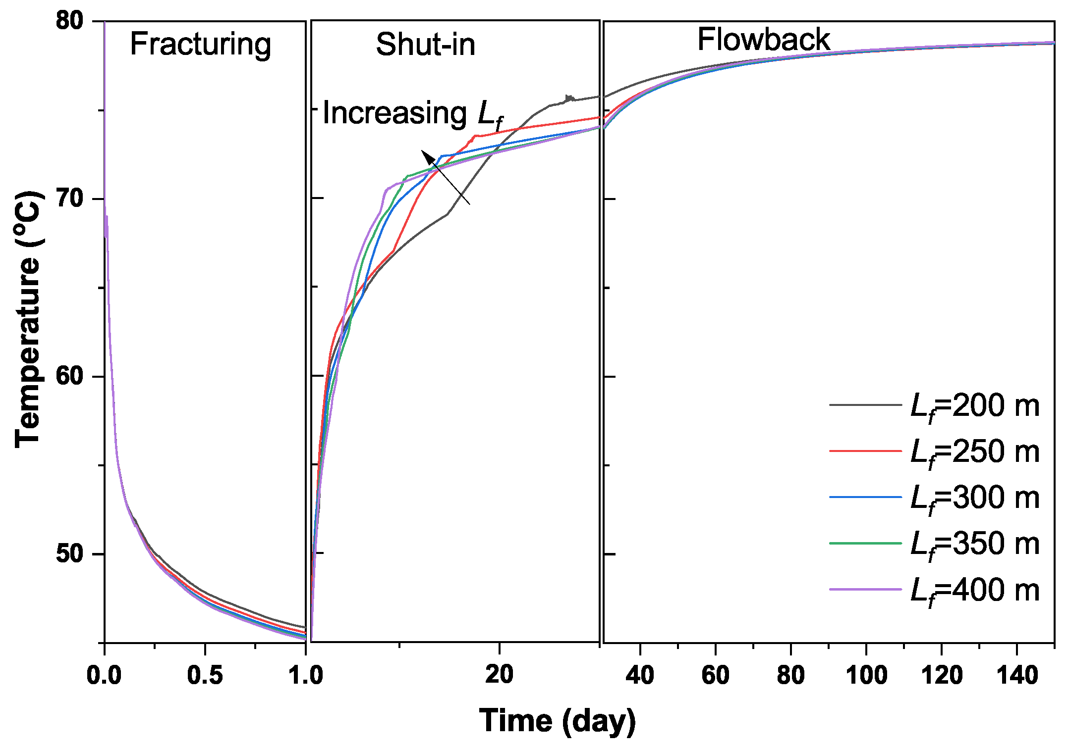
3.3.2. Case 2: Impact of Fracture Length

In this subsection, we investigate the effect of L f on the behaviors of fracture temperature during the fracturing, shut-in, and flowback periods. Five different simulation cases with 200, 250, 300, 350, and 400 m of L f were designed. The values align with the effective fracture length characterized by rate-transient analysis [62,63].
Figure 8 compares various plots of fracture temperature for cases with different L f . In general, L f has a negligible effect on fracture-temperature change during the fracturing period. Simulation cases with a smaller L f show a slower warm-up process during the shut-in period, but a higher fracture temperature at the end of shut-in period. This can be explained by the combined effect of fracture surface area ( A f ) and water volume in fractures: Increasing L f increases A f , which further contributes to a faster warm-up process. On the other hand, more injected water remains in fractures for the cases with longer fractures, which further contributes to a relatively lower fracture temperature at the end of shut-in period.

3.3.3. Case 3: Impact of Thermal Conductivity

In this subsection, we investigate the effect of α on the behaviors of temperature during the fracturing, shut-in, and flowback periods. Therefore, four different simulation cases with 88,992, 148,608, 257,472, and 350,784 J/(m·day·°C) of α were designed. These values align with the variations of α for shales from different basins [64].
Figure 9 compares the profiles of fracture temperature for cases with various α during the periods of fracturing, shut-in, and flowback. Figure 9 shows a higher fracture temperature for the cases with higher α . Mineralogy, porosity and fluid control are among the key factors impacting α of sedimentary rocks [65]. One may further expect a faster warm-up process for gas wells completed in a clay-rich tight reservoir with formation water.

3.3.4. Case 4: Impact of Shut-in Days

In this subsection, we investigate the effect of shut-in days on the behaviors of temperature during the shut-in and flowback periods. Four different simulation cases with 0, 10, 20, 30 days of shut-in days were designed. These shut-in periods correspond to the field practices in different shale reservoirs [16,18,19].
Figure 10 compares fracture temperature for cases with varying shut-in days. Interestingly, these cases show an identical fracture-temperature profile in the early 10 days after the fracturing period. Comparing the gas saturation in fractures ( S a v g ) with shut-in days suggests that the 10-day period corresponds to the period prior to gas breakthrough from matrix into fractures. The identical fracture-temperature profiles among these cases suggest heat conduction remains to be the key mechanism of heat transfer before gas breakthrough. In addition, one may conclude that gas flow from matrix into fracture plays a key role in the fracture-temperature change during the shut-in and flowback periods. After gas breakthrough, the results show a relatively slower warm-up process for cases with a longer shut-in period. After opening well for flowback, an increasing amount of gas is expected to flow from matrix into fractures, accelerating the warm-up process.

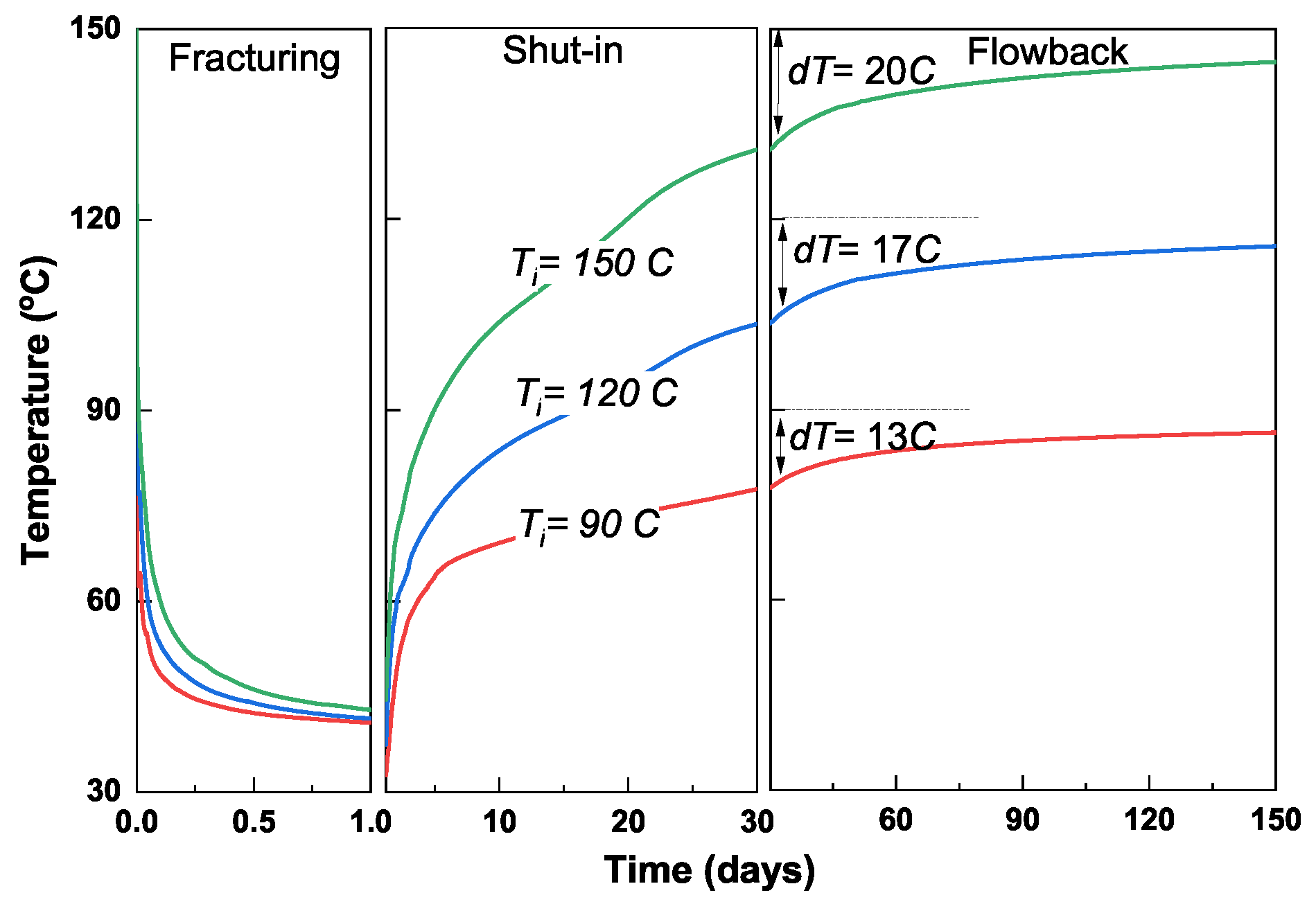
3.3.5. Case 5: Initial Reservoir Temperature

In this subsection, we investigate the effect of T i on the behaviors of temperature during the fracturing, shut-in, and flowback periods. Three different simulation cases with T i = 90, 120 and 150 °C were designed. These values of T i are within the range of formation temperatures for shale reservoirs such as Utica, Bakken, Eagle Ford, and Haynesville (see Figure 1).
Figure 11 compares the fracture-temperature change with different T i . After fracturing treatment, the results show very close values of fracture temperature (at about 40 °C). The cases with a higher T i show a more significant difference between T i and fracture temperature after 30 days of shut-in. This difference is expected to be higher for the well with shorter shut-in days. The results further indicate the wells completed in a relatively hot shale formation may experience a significant change in fracture temperature during flowback, especially for the wells without extended shut-in.

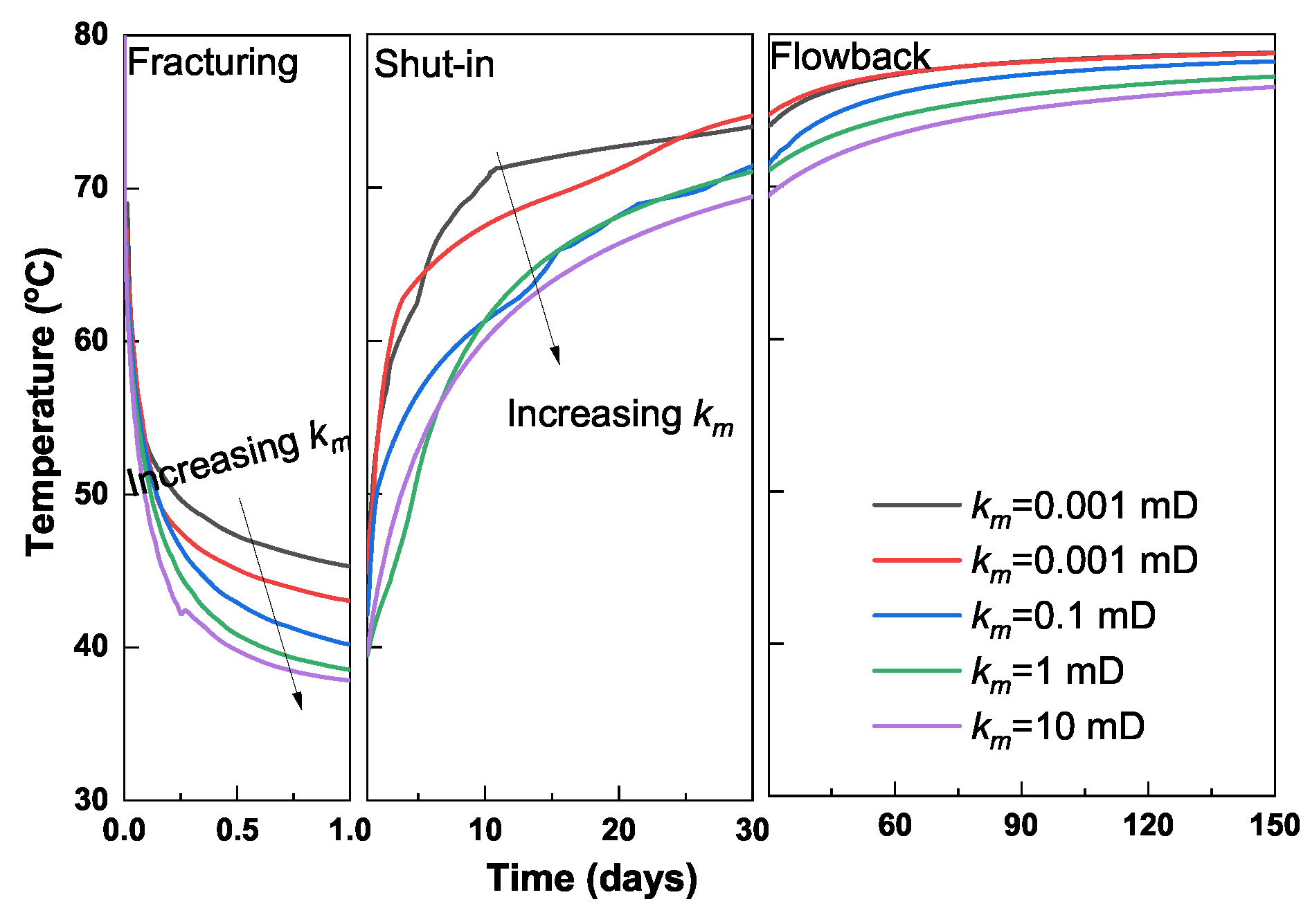
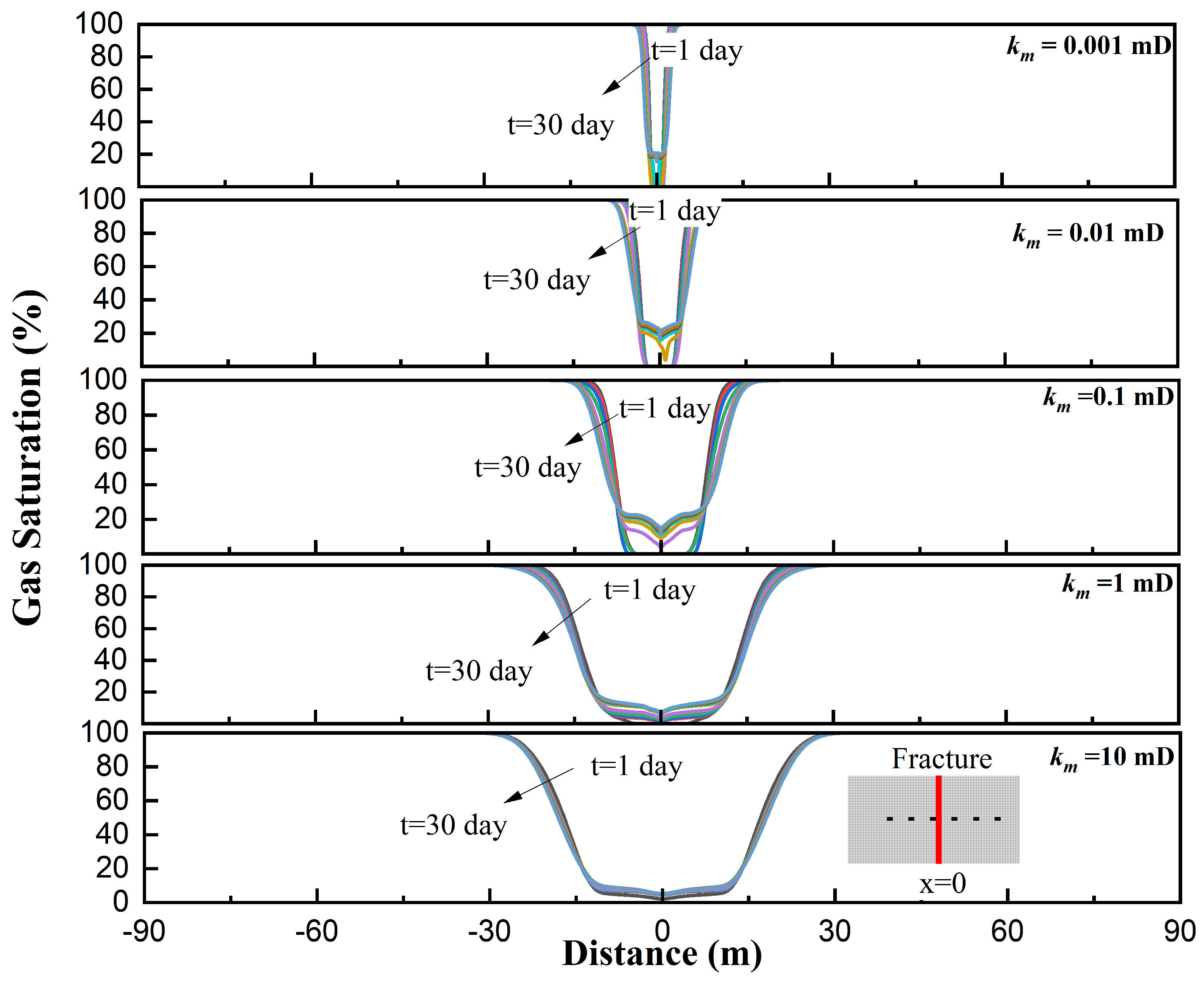
3.3.6. Case 6: Impact of Matrix Permeability

In this subsection, we investigate the effect of k m on the behaviors of temperature during the fracturing, shut-in, and flowback periods. Five different simulation cases with 0.001–10 mD were designed.
Figure 12 compares the fracture-temperature change for cases with different k m . During the fracturing period, we observe a more significant drop in fracture temperature for cases with a larger k m . By contrast, these cases with a larger k m show a relatively faster warm-up process during the shut-in and flowback periods. As shown in Figure A1, increasing k m results in a more significant volume of water lost into matrix, further contributing to an expanded region of matrix cooled down by fracturing water. It then takes a longer time for fractures in these cases to be warmed up during the shut-in and flowback periods. After fracturing treatment, one may thus expect a faster warm-up process for the shale reservoirs with a lower k m .

4. Temperature Impacts Flowback Data Analysis

This section investigates the thermal effect on multiphase-flow modeling during the shut-in and flowback periods. Simulation scenarios are compared to illustrate the effect of temperature on fracture cleanup and early well performance. The results of fracture-volume estimation are also compared to investigate the effect of temperature on flowback data analysis.

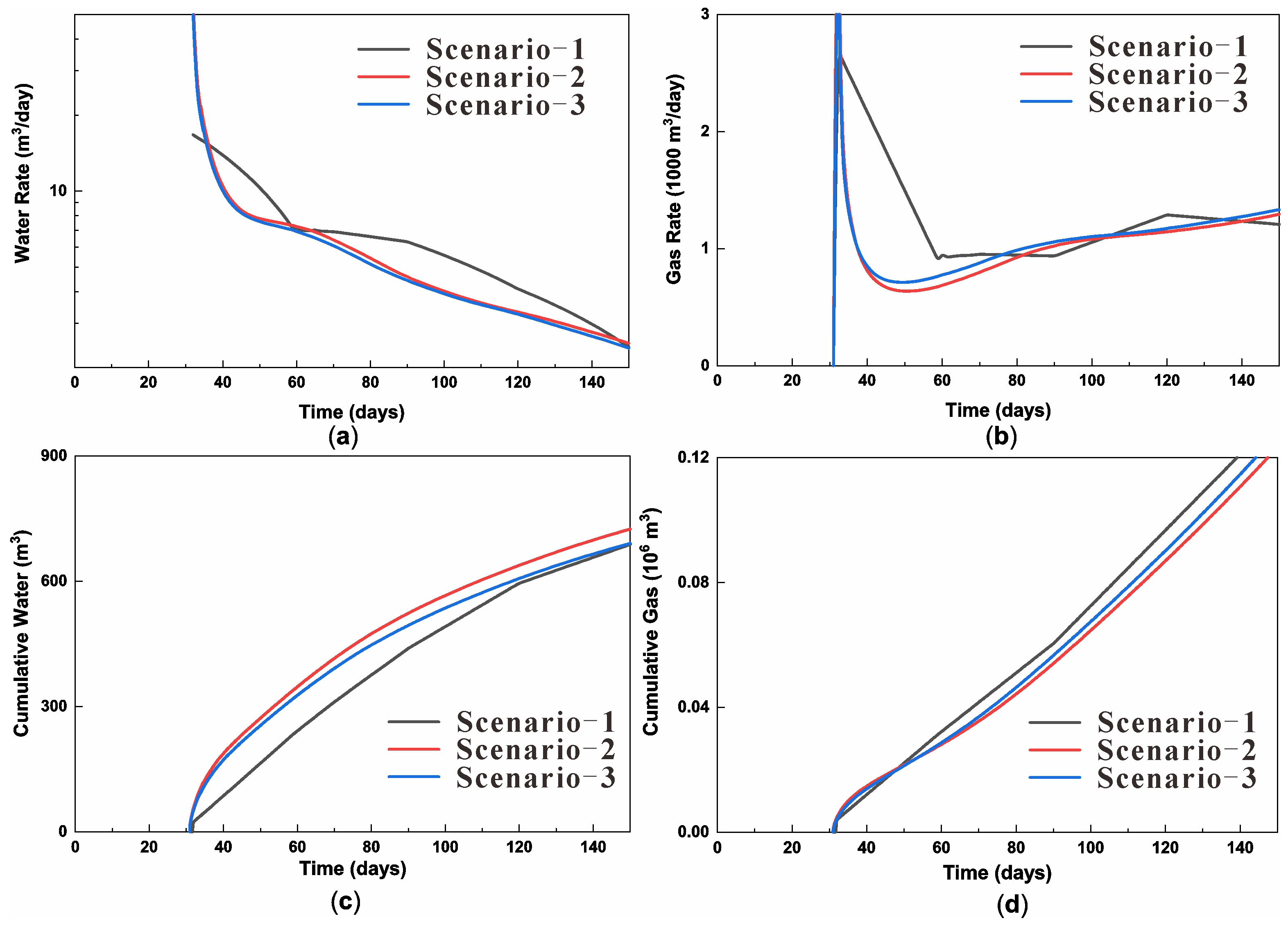
4.1. Flowback Well Performance

Three scenarios of simulation were designed to simulate the fracturing, shut-in, and flowback processes. In Scenario-1, the black-oil model (IMEX) was employed to simulate these processes without considering the thermal effect. In Scenario-2, STARS was employed where fracturing water was injected at the temperature of T i . In Scenario-3, STARS was employed where fracturing water was injected at room temperature. To eliminate the Joule–Tompson effect, the flowing pressure was set at 3000 kPa for these scenarios during the flowback period.
In Figure 13, Scenario-1 shows a relatively lower water production volume and a higher gas production volume compared with Scenarios-2 and -3. The results suggest that not considering the thermal effect may yield an underestimated water production and an overestimated gas production for simulating the shut-in and flowback processes. In addition, Figure 13a,c shows similar water rate and cumulative water volume ( W p ) between Scenarios-2 and -3, implying a negligible effect of temperature on water production. The similar water production volume between Scenarios-2 and -3 may be attributed to the negligible effect of temperature on water mobility.
As shown in Figure 13b,d, Scenario-2 shows a higher gas rate and cumulative gas volume than Scenario-3. The results indicate that not considering the temperature difference between fracturing water and formation rock ( Δ T ) will yield an overestimated gas production. The average gas mobility in Scenario-3 is lower than that in Scenario-2 due to the lower temperature, further contributing to a relatively lower gas production volume. However, Δ T is expected to have negligible effect on gas production at the late period of flowback as the fracture temperature approaches T i . This is supported by the relatively close gas rate after 100 h of flowback (Figure 13b).

4.2. Fracture Cleanup

In this subsection, we investigate the effect of temperature on fracture cleanup during the shut-in and flowback periods. The log-log plot of gas–water ratio (GWR) versus cumulative gas volume ( G p ) is employed to diagnose fracture cleanup [32]. In addition, this subsection investigates the effect of T i on fracture cleanup by comparing the changes in S a v g for simulation cases with various T i .
Figure 14a shows the diagnostic plot of GWR versus G p for Scenarios-2 and -3 (refer to Section 4.1). The results show a relatively higher GWR in Scenario-2 than that in Scenario-3, suggesting that without considering Δ T leads to an optimistic fracture cleanup. GWR is mainly a function of water saturation in fractures [66]. In Figure 14b, we compare the the changes in S a v g for Scenarios-2 and -3. The results show a relatively higher S a v g in Scenario-2 than that in Scenario-3, supporting that it may yield an optimistic fracture cleanup if the shut-in and flowback processes were simulated without considering Δ T .
Figure 15 compares the water saturation in fractures for Scenarios-1 and -3 (refer to Section 4.1) at the end of shut-in, flowback, and long-term production. After 1000 days of production, Scenario-3 shows a relatively higher water saturation in fractures compared with Scenario-1. One may expect that not considering the thermal effects yields an overestimated recovery of fracturing water during long-term production.
Figure 16 compares the profiles of S a v g for simulation cases with various T i . At a higher T i , the results show a higher S a v g during the shut-in and flowback periods. In addition, simulation cases with a higher T i show an earlier gas breakthrough during the shut-in period. The difference in S a v g among these cases can be attributed to the effect of temperature on imbibition during the shut-in period. Experimental studies indicated that increasing temperature decreases the surface tension between water and gas [67,68,69,70]. The change in gas saturation during shut-in is mainly driven by capillary force, which is a function of surface tension further relating to temperature. As supported by the results in Section 3.3.5, increasing T i increases the difference between T i and fracture temperature (Figure 11). This temperature difference is recommended to be considered for future studies of imbibition during the shut-in period, especially for gas wells completed in shales with a relatively high T i .
During the flowback period, one drive mechanism of fracture cleanup is gas vaporizing water [71,72]. This mechanism is described by water in fractures evaporated by flowing gas, which becomes under-saturated with pressure depletion during flowback. However, the solubility of gas in water is a function of temperature. The fluid temperature in fractures is expected to be relatively low during early flowback for the shale gas wells without extended shut-in days. Among such shale gas wells, fracture cleanup driven by gas vaporizing water might thus be negligible due to the relatively low temperature.

4.3. On Fracture-Volume Estimation

In this subsection, we qualitatively investigate the effect of temperature on flowback data analysis. As described in Appendix B, we applied Alkouh et al.’s [15] method of flowback data analysis to estimate effective fracture volume for Scenarios-1, -2, and -3 (refer to Section 4.1).
Figure 17 shows the cartesian plot of rate-normalized pressure ( R N P ) versus material balance time ( M B T ) (refer to Equations (A1) and (A2) in Appendix B). Scenario-1 shows a larger slope (m) between R N P and M B T than Scenarios-2 and -3. In addition, the total compressibility in Scenario-1 is expected to be higher than that in Scenarios-2 and -3 due to the relatively higher S a v g (refer to Equation (A4)). According to Equation (A3), the estimated fracture-volume in Scenario-1 is thus lower than that in Scenarios-2 and -3.
In Figure 17, the fitting results of Scenarios-2 and -3 show relatively close value of slope between R N P and M B T . However, in Figure 16, Scenario-2 shows a higher S a v g compared with Scenario-3. The estimated fracture volume in Scenario-2 is thus expected to be smaller than that in Scenarios-3. One may conclude that not considering Δ T may yield an overestimated fracture volume.

5. Implications

5.1. On Flowback Chemical Analysis

A relatively high salinity of returned water is commonly reported in shale gas wells [39,73,74,75]. In recent years, models have been developed to describe the salt transfer during the shut-in and flowback periods [40,41,42,76,77]. These models have been applied on field salinity data from Marcellus [41,42], Horn River [39,40,42], and Haynesville [42] shales to characterize fractures. However, most of these models assume a constant diffusion coefficient for the mass transfer of ions between formation rock (and/or connate water) and fracturing water, without considering the effect of temperature change during the shut-in and flowback periods. This study suggests that wells may go through a significant change in fracture temperature during the shut-in and flowback periods. The temperature change may significantly affect the outputs when applying these models on field data. This is supported by a recent experimental work which indicated the mass transfer of ions is sensitive to temperature [78]. It is thus recommended to consider this temperature change for modeling the flowback behaviors of salinity for future works.

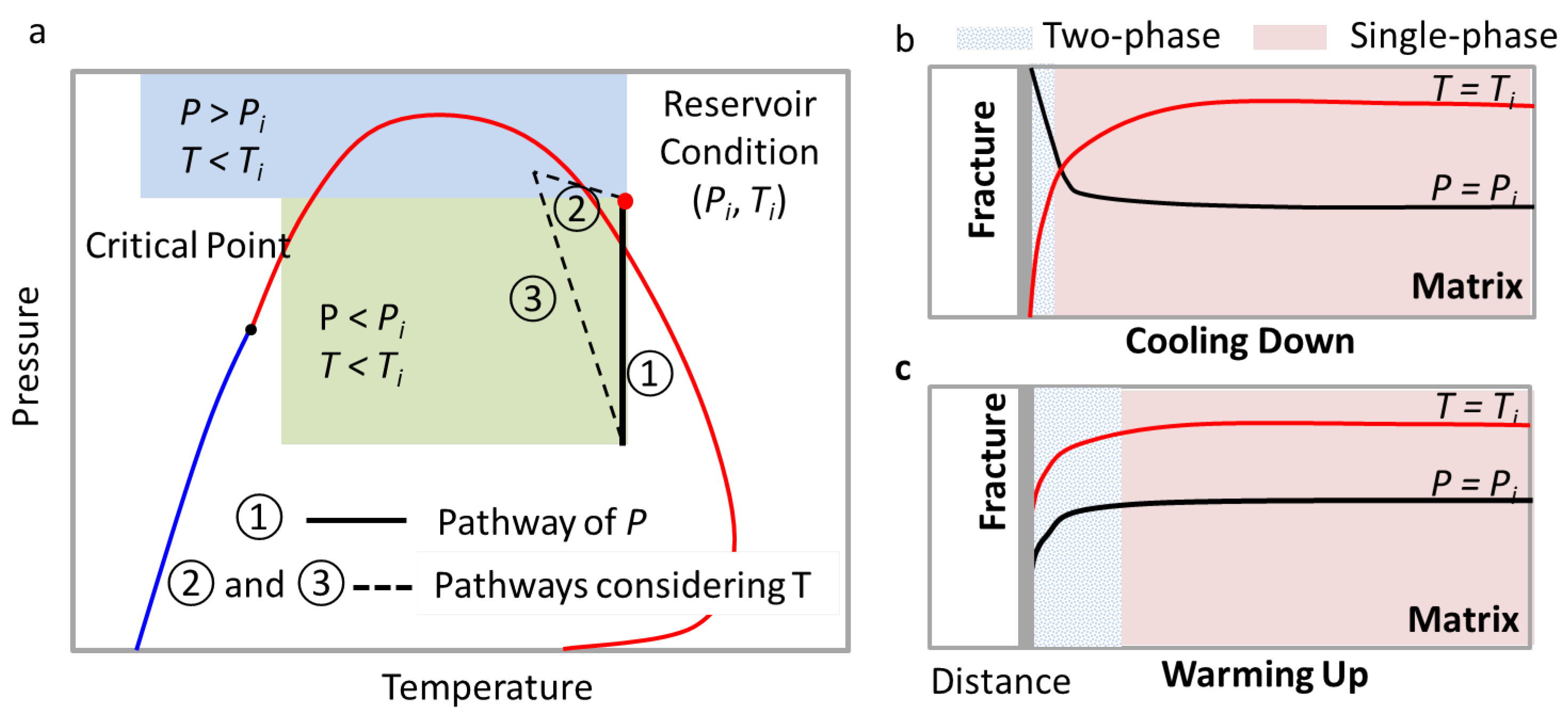
5.2. On Phase Behaviors of Gas-Condensate Wells

Gas-condensate production has been reported from wells completed in Eagle Ford [79], Woodford [80], Duvernay [81], and Montney formations [82,83]. Flowback data from lean-gas wells completed in the Woodford formation have shown condensate production after about 10 days of flowback [80]. Condensate banking can be a critical concern of formation damage for these gas wells if bottomhole pressure drops below the critical pressure during flowback. Managing pressure drawdown through optimizing choke size is the key to eliminate the early condensate banking.
As illustrated by Figure 18, gas-condensate wells may go through a process of pressure change, but also temperature change during the fracturing, shut-in, and flowback periods. This study indicated that the temperature change at the interface of matrix and fracture can be over 40 °C (see Figure 6). This temperature change can be even higher in deep shale reservoirs with a higher T i . Condensate banking may occur at the fracture-matrix interface due to this temperature change for gas-condensate reservoirs where the initial temperature and pressure are close to the phase envelope of reservoir fluids. As such, the pathway of temperature change is also recommended to be considered for the flowback choke-size management of gas-condensate wells.

6. Limitations and Recommendation for Future Studies

This study simulated the fracturing treatment by assuming it as a process of water injection. Fracture growth, typically as a function of time [85], was not considered in this study. In addition, the period of one-day injection can be longer than that in field practice, which generally takes up to several hours for a single fracturing stage. However, the temperature change during the fracturing period obtained from this study is within the ranges reported by DST measurement and modeling studies [4,58,59,60,61]. We thus expect that treating the fracturing process as water injection will not significantly bias our key conclusions on the the fracture temperature during the shut-in and flowback periods. However, expressing fracture growth as a function of time is recommended for future studies to better characterize the temperature behaviors during the fracturing period.
In this study, a planar fracture was assumed to simulate the temperature behaviors in hydraulic fractures for shale gas wells. However, intensive natural fractures are commonly reported in shales [86]. Fracture networks in shale can be quite complex due to the reactivation of natural fractures by hydraulic fracturing. Also, studies suggest that most fracturing water remains in natural fractures after the fracturing treatment [47,87]. The results of temperature change may thus be influenced by the simplified fracture geometry for shale gas wells. The reactivated natural fractures can significantly increase the fracture surface area, further accelerating the warm-up process. Future studies should extend the work by considering natural fractures in the models, and investigate the effect of fracture complexity on the temperature behaviors during the shut-in and flowbak periods.

7. Conclusions

This work conducted simulations to investigate the behaviors of temperature during the fracturing, shut-in, and flowback periods of shale gas wells. The changes of temperature with space and time were characterized through numerical simulations. Sensitivity analysis was then conducted to investigate the effect of fracture and matrix parameters on the temperature change. In addition, this work investigated the effect of temperature change on flowback data analysis through a comparative analysis of various simulation scenarios. The main conclusions are summarized as follows:
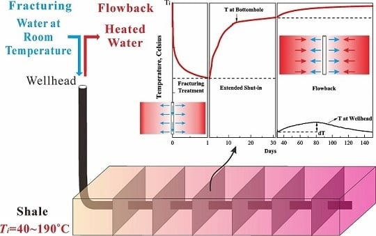
  • Formation is cooled down during the fracturing period. The cool-down region in formation expands with time. However, the change in formation temperature is constrained within the area near the matrix–fracture interface during the shut-in and flowback periods. Fractures are warmed up after the fracturing treatment. The warm-up process mainly occurs during the early shut-in period. Wells without any extended shut-in days can experience a significant increase in fracture temperature during the flowback period.
  • Gas flow from matrix into fracture plays a key role in the fracture-temperature change during the shut-in and flowback periods. Sensitivity analysis indicates that fractures with a smaller width and larger length generally contribute to an accelerated warm-up process, whereas increasing matrix permeability contributes to a slower warm-up process. In addition, the change in fracture temperature is highly related to thermal conductivity of formation rock and initial reservoir temperature.
  • Without considering the temperature change, flowback simulation may yield an overestimated gas production and underestimated water production. The change in fracture temperature also affects the gas saturation in fractures during shut-in, which further affects the process of fracture cleanup during flowback. Flowback data analysis without considering the temperature change may yield an overestimated fracture volume. In addition, it is recommended to consider the thermal effect for flowback chemical analysis and flowback drawdown management.

Author Contributions

S.Y., F.L., and Y.F. conceived and designed the study. S.Y., Z.L., and Y.F. wrote the paper. K.W., L.Z. and Y.L. reviewed and edited the manuscript. All authors read and approved the manuscript.

Acknowledgments

The authors thank for the funding supports from the Fundamental Research Funds of the Central Universities (2-9-2018-210) and National Science and Technology Major Project of China (Grant Nos. 2017ZX05030-003 and 2017ZX05009-005).

Conflicts of Interest

The authors declare no conflict of interest.

Data Availability

All of the data used to support the findings of this study are included in the article.

Abbreviations

AFracture surface area
B w Water formation factor
C t Total compressibility of water, gas, and fracture
V e f Effective fracture volume
T i Initial formation temperature
T 2 Fracture temperature at the end of fracturing operation
R N P Rate-normalized pressure
M B T Material balance time
P w f Flowing pressure at bottomhole
P i Initial reservoir pressure
q w Water rate
q g Gas rate
W p Cumulative water volume
G p Cumulative gas volume
α Thermal conductivity

Appendix A. Gas-Saturation Profiles for Varying km

Figure A1. Comparison of gas-saturation profiles in the formation (dash-line) perpendicular to the fracture wall (red solid-line) for simulation cases with matrix permeability varying from 0.001 to 10 md.
Energies 12 03751 g0a1

Appendix B. Alkouh et al. (2014)’s Method

According to Alkouh et al. [15], the rate-normalized pressure of water and material-balance time are defined by:
R N P = P i P w f q w
M B T = W p q w
where P i is the initial reservoir pressure, k P a ; and P w f is the bottomhole pressure, k P a .
The relationship for estimating fracture volume is described by:
V e f = B w C t · m
where m is the slope between R N P and M B T and C t defines the total compressibility of gas, water, and fracture as:
C t = C f + S a v g · C g + S w · C w
where C f , C g , and C w represent for the compressibility of fracture, gas, and water, respectively; and S a v g is the average gas saturation in fractures.

References

  1. Estrada, J.M.; Bhamidimarri, R. A review of the issues and treatment options for wastewater from shale gas extraction by hydraulic fracturing. Fuel 2016, 182, 292–303. [Google Scholar] [CrossRef]
  2. Bahr, H.A.; Weiss, H.J.; Bahr, U.; Hofmann, M.; Fischer, G.; Lampenscherf, S.; Balke, H. Scaling behavior of thermal shock crack patterns and tunneling cracks driven by cooling or drying. J. Mech. Phys. Solids 2010, 58, 1411–1421. [Google Scholar] [CrossRef]
  3. Tarasovs, S.; Ghassemi, A. Self-similarity and scaling of thermal shock fractures. Phys. Rev. E 2014, 90, 012403. [Google Scholar] [CrossRef] [PubMed] [Green Version]
  4. Enayatpour, S.; van Oort, E.; Patzek, T. Thermal cooling to improve hydraulic fracturing efficiency and hydrocarbon production in shales. J. Nat. Gas Sci. Eng. 2019, 62, 184–201. [Google Scholar] [CrossRef]
  5. Gao, Q.; Tao, J.; Hu, J.; Yu, X.B. Laboratory study on the mechanical behaviors of an anisotropic shale rock. J. Rock Mech. Geotech. Eng. 2015, 7, 213–219. [Google Scholar] [CrossRef] [Green Version]
  6. Qiu, P.; Hu, R.; Hu, L.; Liu, Q.; Xing, Y.; Yang, H.; Qi, J.; Ptak, T. A Numerical Study on Travel Time Based Hydraulic Tomography Using the SIRT Algorithm with Cimmino Iteration. Water 2019, 11, 909. [Google Scholar] [CrossRef]
  7. Sookprasong, P.; Gill, C.C.; Hurt, R.S. Lessons learned from das and dts in multicluster, multistage horizontal well fracturing: Interpretation of hydraulic fracture initiation and propagation through diagnostics. In Proceedings of the IADC/SPE Asia Pacific Drilling Technology Conference, Bangkok, Thailand, 25–27 August 2014. [Google Scholar]
  8. Ugueto, G.A.; Huckabee, P.T.; Molenaar, M.M. Challenging Assumptions About Fracture Stimulation Placement Effectiveness Using Fiber Optic Distributed Sensing Diagnostics: Diversion, Stage Isolation and Overflushing. In Proceedings of the SPE Hydraulic Fracturing Technology Conference, The Woodlands, TX, USA, 3–5 February 2015. [Google Scholar]
  9. Ugueto, C.; Gustavo, A.; Huckabee, P.T.; Molenaar, M.M.; Wyker, B.; Somanchi, K. Perforation cluster efficiency of cemented plug and perf limited entry completions; Insights from fiber optics diagnostics. In Proceedings of the SPE Hydraulic Fracturing Technology Conference, The Woodlands, TX, USA, 9–11 February 2016. [Google Scholar]
  10. Sierra, J.R.; Kaura, J.D.; Gualtieri, D.; Glasbergen, G.; Sarker, D.; Johnson, D. DTS monitoring of hydraulic fracturing: Experiences and lessons learned. In Proceedings of the SPE Annual Technical Conference and Exhibition, Denver, CO, USA, 21–24 September 2008. [Google Scholar]
  11. Holley, E.H.; Molenaar, M.M.; Fidan, E.; Banack, B. Interpreting uncemented multistage hydraulic-fracturing completion effectiveness by use of fiber-optic DTS injection data. SPE Drill. Complet. 2013, 28, 243–253. [Google Scholar] [CrossRef]
  12. Beck, G.; Verma, S. Development and Field Testing Novel Natural Gas (NG) Surface Process Equipment for Replacement of Water as Primary Hydraulic Fracturing Fluid. In Proceedings of the Carbon Storage and Oil and Natural Gas Technologies Review Meeting, Pittsburgh, PA, USA, 16–18 August 2016. [Google Scholar]
  13. Cheng, Y. Impact of water dynamics in fractures on the performance of hydraulically fractured wells in gas shale reservoirs. In Proceedings of the SPE International Symposium and Exhibition on Formation Damage Control, Lafayette, LA, USA, 10–12 February 2010. [Google Scholar]
  14. Cheng, Y. Impact of Water Dynamics in Fractures on the Performance of Hydraulically Fractured Wells in Gas-Shale Reservoirs. J. Can. Pet. Technol. 2012, 51, 143–151. [Google Scholar] [CrossRef]
  15. Alkouh, A.; McKetta, S.; Wattenbarger, R.A. Estimation of Effective-Fracture Volume Using Water-Flowback and Production Data for Shale-Gas Wells. J. Can. Pet. Technol. 2014, 53, 290–303. [Google Scholar] [CrossRef]
  16. Ghanbari, E.; Dehghanpour, H. The fate of fracturing water: A field and simulation study. Fuel 2016, 163, 282–294. [Google Scholar] [CrossRef]
  17. Noe, S.; Crafton, J. Factors Affecting Early Well Productivity in Six Shale Plays. In Proceedings of the SPE Annual Technical Conference and Exhibition, New Orleans, LA, USA, 30 September–2 October 2013. [Google Scholar]
  18. Edwards, R.W.; Celia, M.A. Shale gas well, hydraulic fracturing, and formation data to support modeling of gas and water flow in shale formations. Water Resour. Res. 2018, 54, 3196–3206. [Google Scholar] [CrossRef]
  19. Bertoncello, A.; Wallace, J.; Blyton, C.; Honarpour, M.M.; Kabir, S. Imbibition and Water Blockage in Unconventional Reservoirs: Well-Management Implications During Flowback and Early Production. SPE Reserv. Eval. Eng. 2014, 17, 497–506. [Google Scholar] [CrossRef]
  20. Wang, Q.; Guo, B.; Gao, D. Is Formation Damage an Issue in Shale Gas Development? In Proceedings of the SPE International Symposium and Exhibition on Formation Damage Control, Lafayette, LA, USA, 15–17 February 2012. [Google Scholar]
  21. Cao, P.; Liu, J.; Leong, Y.K. A multiscale-multiphase simulation model for the evaluation of shale gas recovery coupled the effect of water flowback. Fuel 2017, 199, 191–205. [Google Scholar] [CrossRef]
  22. Wijaya, N.; Sheng, J.J. Effect of desiccation on shut-in benefits in removing water blockage in tight water-wet cores. Fuel 2019, 244, 314–323. [Google Scholar] [CrossRef]
  23. Lai, F.; Li, Z.; Wang, Y. Impact of water blocking in fractures on the performance of hydraulically fractured horizontal wells in tight gas reservoir. J. Pet. Sci. Eng. 2017, 156, 134–141. [Google Scholar] [CrossRef]
  24. Fakcharoenphol, P.; Torcuk, M.; Kazemi, H.; Wu, Y.S. Effect of shut-in time on gas flow rate in hydraulic fractured shale reservoirs. J. Nat. Gas Sci. Eng. 2016, 32, 109–121. [Google Scholar] [CrossRef] [Green Version]
  25. Edwards, R.W.; Doster, F.; Celia, M.A.; Bandilla, K.W. Numerical modeling of gas and water flow in shale gas formations with a focus on the fate of hydraulic fracturing fluid. Environ. Sci. Technol. 2017, 51, 13779–13787. [Google Scholar] [CrossRef]
  26. Birdsell, D.T.; Rajaram, H.; Dempsey, D.; Viswanathan, H.S. Hydraulic fracturing fluid migration in the subsurface: A review and expanded modeling results. Water Resour. Res. 2015, 51, 7159–7188. [Google Scholar] [CrossRef]
  27. Taherdangkoo, R.; Tatomir, A.; Taylor, R.; Sauter, M. Numerical investigations of upward migration of fracking fluid along a fault zone during and after stimulation. Energy Procedia 2017, 125, 126–135. [Google Scholar] [CrossRef]
  28. Taherdangkoo, R.; Tatomir, A.; Anighoro, T.; Sauter, M. Modeling fate and transport of hydraulic fracturing fluid in the presence of abandoned wells. J. Contam. Hydrol. 2019, 221, 58–68. [Google Scholar] [CrossRef]
  29. Lan, Q.; Ghanbari, E.; Dehghanpour, H. Water loss versus soaking time: Spontaneous imbibition in tight rocks. In Proceedings of the SPE/EAGE European Unconventional Resources Conference and Exhibition, Vienna, Austria, 25–27 February 2014. [Google Scholar]
  30. Makhanov, K.; Habibi, A.; Dehghanpour, H.; Kuru, E. Liquid uptake of gas shales: A workflow to estimate water loss during shut-in periods after fracturing operations. J. Unconv. Oil Gas Resour. 2014, 7, 22–32. [Google Scholar] [CrossRef]
  31. Crafton, J.W. Modeling Flowback Behavior or Flowback Equals “Slowback”. In Proceedings of the SPE Shale Gas Production Conference, Fort Worth, TX, USA, 16–18 November 2008. [Google Scholar]
  32. Ilk, D.; Currie, S.M.; Symmons, D.; Broussard, N.J.; Blasingame, T.A. A Comprehensive Workflow for Early Analysis and Interpretation of Flowback Data from wells in Tight Gas/Shale Reservoir Systems. In Proceedings of the SPE Annual Technical Conference and Exhibition, Florence, Italy, 20–22 September 2010. [Google Scholar]
  33. Ezulike, D.O.; Dehghanpour, H. A model for simultaneous matrix depletion into natural and hydraulic fracture networks. J. Nat. Gas Sci. Eng. 2014, 16, 57–69. [Google Scholar] [CrossRef]
  34. Abbasi, M.A.; Dehghanpour, H.; Hawkes, R.V. Flowback Analysis for Fracture Characterization. In Proceedings of the SPE Canadian Unconventional Resources Conference, Calgary, AB, Canada, 30 October–1 November 2012. [Google Scholar]
  35. Clarkson, C.R. Modeling 2-Phase Flowback of Multi-Fractured Horizontal Wells Completed in Shale. In Proceedings of the SPE Canadian Unconventional Resources Conference, Calgary, AB, Canada, 30 October–1 November 2012. [Google Scholar]
  36. Williams-Kovacs, J.; Clarkson, C. Stochastic Modeling of Multi-Phase Flowback From Multi-Fractured Horizontal Tight Oil Wells. In Proceedings of the SPE Unconventional Resources Conference-Canada, Calgary, AB, Canada, 5–7 November 2013. [Google Scholar]
  37. Abbasi, M.A.; Ezulike, D.O.; Dehghanpour, H.; Hawkes, R.V. A Comparative Study of Flowback Rate and Pressure Transient Behavior in Multifractured Horizontal Wells Completed in Tight Gas and Oil Reservoirs. J. Nat. Gas Sci. Eng. 2014, 17, 82–93. [Google Scholar] [CrossRef]
  38. Xu, M.; Dehghanpour, H. Advances in Understanding Wettability of Gas Shales. Energy Fuels 2014, 28, 4362–4375. [Google Scholar] [CrossRef]
  39. Bearinger, D. Message in a Bottle. In Proceedings of the Unconventional Resources Technology Conference, Denver, CO, USA, 12–14 August 2013. [Google Scholar]
  40. Zolfaghari, A.; Dehghanpour, H.; Ghanbari, E.; Bearinger, D. Fracture characterization using flowback salt-concentration transient. SPE J. 2016, 21, 233–244. [Google Scholar] [CrossRef]
  41. Balashov, V.N.; Engelder, T.; Gu, X.; Fantle, M.S.; Brantley, S.L. A model describing flowback chemistry changes with time after Marcellus Shale hydraulic fracturing. AAPG Bull. 2015, 99, 143–154. [Google Scholar] [CrossRef]
  42. Merry, H.; Ehlig-Economides, C.; Wei, P. Model for a Shale Gas Formation with Salt-Sealed Natural Fractures. In Proceedings of the SPE Annual Technical Conference and Exhibition, Houston, TX, USA, 28–30 September 2015. [Google Scholar]
  43. Carpenter, C. Model for a Shale-Gas Formation with Salt-Sealed Natural Fractures. J. Pet. Technol. 2016, 68, 62–64. [Google Scholar] [CrossRef]
  44. Wang, J.Y.; Holditch, S.; McVay, D. Modeling fracture-fluid cleanup in tight-gas wells. SPE J. 2010, 15, 783–793. [Google Scholar] [CrossRef]
  45. Wang, T.; Tian, S.; Li, G.; Sheng, M.; Ren, W.; Liu, Q.; Tan, Y.; Zhang, P. Experimental study of water vapor adsorption behaviors on shale. Fuel 2019, 248, 168–177. [Google Scholar] [CrossRef]
  46. Mullen, J. Petrophysical characterization of the Eagle Ford Shale in south Texas. In Proceedings of the Canadian Unconventional Resources and International Petroleum Conference, Calgary, AB, Canada, 19–21 October 2010. [Google Scholar]
  47. Agrawal, S.; Sharma, M.M. Practical insights into liquid loading within hydraulic fractures and potential unconventional gas reservoir optimization strategies. J. Unconv. Oil Gas Resour. 2015, 11, 60–74. [Google Scholar] [CrossRef] [Green Version]
  48. Agrawal, S.; Sharma, M.M. Impact of Liquid Loading in Hydraulic Fractures on Well Productivity. In Proceedings of the SPE Hydraulic Fracturing Technology Conference, The Woodlands, TX, USA, 4–6 February 2013. [Google Scholar]
  49. Korson, L.; Drost-Hansen, W.; Millero, F.J. Viscosity of water at various temperatures. J. Phys. Chem. 1969, 73, 34–39. [Google Scholar] [CrossRef]
  50. Korosi, A.; Fabuss, B.M. Viscosity of liquid water from 25 to 150. degree. measurements in pressurized glass capillary viscometer. Anal. Chem. 1968, 40, 157–162. [Google Scholar] [CrossRef]
  51. Carmichael, L.; Berry, V.; Sage, B. Viscosity of Hydrocarbons. Methane. J. Chem. Eng. Data 1965, 10, 57–61. [Google Scholar] [CrossRef]
  52. Zhao, J.; Peng, Y.; Li, Y.; Tian, Z.; Fu, D. A semi-analytic model of wellbore temperature field based on double-layer unsteady heat conducting process. Nat. Gas Ind. 2016, 36, 68–75. [Google Scholar]
  53. Ramires, M.L.; Nieto de Castro, C.A.; Nagasaka, Y.; Nagashima, A.; Assael, M.J.; Wakeham, W.A. Standard reference data for the thermal conductivity of water. J. Phys. Chem. Ref. Data 1995, 24, 1377–1381. [Google Scholar] [CrossRef]
  54. Golubev, I. A bicalorimeter for determining the thermal conductivity of gases and liquids at high pressures and different temperatures. Teploenergetika 1963, 12, 78–82. [Google Scholar]
  55. Fontanilla, J.P.; Aziz, K. Prediction of bottom-hole conditions for wet steam injection wells. J. Can. Pet. Technol. 1982, 21. [Google Scholar] [CrossRef]
  56. Beggs, D.H.; Brill, J.P. A study of two-phase flow in inclined pipes. J. Pet. Technol. 1973, 25, 607–617. [Google Scholar] [CrossRef]
  57. Fontanilla, J.P. A Mathematical Model for the Prediction of Wellbore Heat Loss and Pressure Drop in Steam Injection Wells. Master’s Thesis, University of Calgary, Calgary, AB, Canada, 1980. [Google Scholar]
  58. Zhang, S.; Zhu, D. Efficient Flow Rate Profiling for Multiphase Flow in Horizontal Wells Using Downhole Temperature Measurement. In Proceedings of the International Petroleum Technology Conference, Beijing, China, 26–28 March 2019. [Google Scholar]
  59. Cui, J.; Yang, C.; Zhu, D.; Datta-Gupta, A. Fracture diagnosis in multiple-stage-stimulated horizontal well by temperature measurements with fast marching method. SPE J. 2016, 21, 2–289. [Google Scholar] [CrossRef]
  60. Yoshida, N. Modeling and Interpretation of Downhole Temperature in a Horizontal Well with Multiple Fractures. Ph.D. Thesis, Texas A & M University, College Station, TX, USA, 2016. [Google Scholar]
  61. Yoshida, N.; Hill, A.D.; Zhu, D. Comprehensive Modeling of Downhole Temperature in a Horizontal Well with Multiple Fractures. SPE J. 2018, 23. [Google Scholar] [CrossRef]
  62. Barree, R.D.; Cox, S.A.; Gilbert, J.V.; Dobson, M.L. Closing the gap: Fracture half length from design, buildup, and production analysis. SPE Prod. Facil. 2005, 20, 274–285. [Google Scholar] [CrossRef]
  63. Bybee, K. Resolving Created, Propped, and Effective Hydraulic-Fracture Length. J. Pet. Technol. 2009, 61, 58–60. [Google Scholar] [CrossRef]
  64. Čermák, V.; Rybach, L. Thermal conductivity and specific heat of minerals and rocks. In Landolt-Börnstein: Numerical Data and Functional Relationships in Science and Technology; New Series, Group V (Geophysics and Space Research), Physical Properties of Rocks; Angenheister, G., Ed.; Springer: Berlin/Heidelberg, Germany, 1982; Volume Ia, pp. 305–343. [Google Scholar]
  65. Brigaud, F.; Vasseur, G. Mineralogy, porosity and fluid control on thermal conductivity of sedimentary rocks. Geophys. J. Int. 1989, 98, 525–542. [Google Scholar] [CrossRef] [Green Version]
  66. Ghanbari, E.; Dehghanpour, H. Impact of Rock Fabric on Water Imbibition and Salt Diffusion in Gas Shales. Int. J. Coal Geol. 2015, 138, 55–67. [Google Scholar] [CrossRef]
  67. Jennings, H.Y., Jr.; Newman, G.H. The effect of temperature and pressure on the interfacial tension of water against methane-normal decane mixtures. Soc. Pet. Eng. J. 1971, 11, 171–175. [Google Scholar] [CrossRef]
  68. Rushing, J.A.; Newsham, K.E.; Van Fraassen, K.C.; Mehta, S.A.; Moore, G.R. Laboratory measurements of gas-water interfacial tension at HP/HT reservoir conditions. In Proceedings of the CIPC/SPE Gas Technology Symposium 2008 Joint Conference, Calgary, AB, Canada, 16–19 June 2008. [Google Scholar]
  69. Shariat, A. Measurement and Modeling Gas-Water Interfacial Tension at High Pressure/High Temperature Conditions. Ph.D. Thesis, University of Calgary, Calgary, AB, Canada, 2014. [Google Scholar]
  70. Babadagli, T.; Hatiboglu, C.U. Analysis of counter-current gas–water capillary imbibition transfer at different temperatures. J. Pet. Sci. Eng. 2007, 55, 277–293. [Google Scholar] [CrossRef]
  71. Zhang, Y.; Ehlig-Economides, C. Accounting for remaining injected fracturing fluid in shale gas wells. In Proceedings of the Unconventional Resources Technology Conference, Denver, CO, USA, 25–27 August 2014; pp. 2365–2377. [Google Scholar]
  72. Mahadevan, J.; Sharma, M.M.; Yortsos, Y.C. Evaporative cleanup of water blocks in gas wells. SPE J. 2007, 12, 209–216. [Google Scholar] [CrossRef]
  73. Blauch, M.E.; Myers, R.R.; Moore, T.; Lipinski, B.A.; Houston, N.A. Marcellus shale post-frac flowback waters—Where is all the salt coming from and what are the implications? In Proceedings of the SPE Eastern Regional Meeting, Charleston, WV, USA, 23–25 September 2009. [Google Scholar]
  74. Haluszczak, L.O.; Rose, A.W.; Kump, L.R. Geochemical evaluation of flowback brine from Marcellus gas wells in Pennsylvania, USA. Appl. Geochem. 2013, 28, 55–61. [Google Scholar] [CrossRef]
  75. Hayes, T.D. Sampling and Analysis of Water Streams Associated with the Development of Marcellus Shale Gas; Gas Technology Institute: Des Plaines, IL, USA, 2009. [Google Scholar]
  76. Phan, T.T.; Vankeuren, A.N.P.; Hakala, J.A. Role of water- rock interaction in the geochemical evolution of Marcellus Shale produced waters. Int. J. Coal Geol. 2018, 191, 95–111. [Google Scholar] [CrossRef]
  77. Vazquez, O.; McCartney, R.A.; Mackay, E. Produced-Water-Chemistry History Matching Using a 1D Reactive Injector/Producer Reservoir Model. SPE Prod. Oper. 2013, 28, 369–375. [Google Scholar]
  78. Zolfaghari, A.; Dehghanpour, H.; Bearinger, D. Produced Flowback Salts vs. Induced-Fracture Interface: A Field and Laboratory Study. SPE J. 2019. [Google Scholar] [CrossRef]
  79. Tian, Y.; Ayers, W.B.; McCain, D., Jr. The Eagle Ford Shale play, south Texas: Regional variations in fluid types, hydrocarbon production and reservoir properties. In Proceedings of the IPTC 2013: International Petroleum Technology Conference, Beijing, China, 26–28 March 2013. [Google Scholar]
  80. Jones, R.; Pownall, B.; Franke, J. Estimating reservoir pressure from early flowback data. In Proceedings of the Unconventional Resources Technology Conference, Denver, CO, USA, 25–27 August 2014; pp. 2140–2155. [Google Scholar]
  81. Rodriguez, A.; Maldonado, F. Evaluating Pressure Drawdown Strategy for Hydraulically Fracture Shale Gas Condensate Producers. In Proceedings of the SPE Oklahoma City Oil and Gas Symposium, Oklahoma City, OK, USA, 9–10 April 2019. [Google Scholar]
  82. Reynolds, M.; Bachman, R.; Buendia, J.; Peters, W. The full montney—A critical review of well performance by production analysis of over 2000 montney multi-stage fractured horizontal gas wells. In Proceedings of the SPE/CSUR Unconventional Resources Conference, Calgary, AB, Canada, 20–22 October 2015. [Google Scholar]
  83. Fu, Y.; Dehghanpour, H.; Motealleh, S.; Lopez, C.M.; Hawkes, R. Evaluating Fracture Volume Loss During Flowback and Its Relationship to Choke Size: Fastback vs. Slowback. SPE Prod. Oper. 2019, 34, 615–624. [Google Scholar] [CrossRef]
  84. Fan, L.; Harris, B.W.; Jamaluddin, A.; Kamath, J.; Mott, R.; Pope, G.A.; Shandrygin, A.; Whitson, C.H. Understanding gas-condensate reservoirs. Oilfield Rev. 2005, 17, 14–27. [Google Scholar]
  85. Amini, K.; Soliman, M.Y.; House, W.V. A Three-Dimensional Thermal Model for Hydraulic Fracturing. In Proceedings of the SPE Annual Technical Conference and Exhibition, Houston, TX, USA, 28–30 September 2015. [Google Scholar]
  86. Olson, J.E.; Laubach, S.E.; Lander, R.H. Natural fracture characterization in tight gas sandstones: Integrating mechanics and diagenesis. AAPG Bull. 2009, 93, 1535–1549. [Google Scholar] [CrossRef]
  87. Fu, Y.; Dehghanpour, H.; Ezulike, D.O.; Jones, R.S., Jr. Estimating effective fracture pore volume from flowback data and evaluating its relationship to design parameters of multistage-fracture completion. SPE Prod. Oper. 2017, 32, 423–439. [Google Scholar] [CrossRef]
Figure 1. Comparing the range of formation temperature with average formation depth for shale and tight plays in North America (data source: [12]).
Energies 12 03751 g001
Figure 2. Schematics illustrating the model for numerical simulation: (a) the section of reservoir volume between two fracturing stages was selected for this study (modified from [24]); (b) the grid system with dimensions; and (c) the section view of fracture surface wall (in pink).
Energies 12 03751 g002
Figure 3. Schematics illustrating the wellbore model (modified from [55]).
Energies 12 03751 g003
Figure 4. Comparing the bottomhole and wellhead temperature during the fracturing, shut-in, and flowback periods. In the simulation, the bottomhole temperature is represented by the formation temperature at the grid of wellbore. Wellhead temperature is only simulated for the flowback period.
Energies 12 03751 g004
Figure 5. Comparing the temperature profiles along the fracture wall (refer to Figure 2c) with distance away from wellbore ( x = 0 ) during the fracturing (top), shut-in (middle), and flowback (bottom) periods. The positive and negative values of x represent the distance away from wellbore at different sides. Each color represents the temperature profile at the different time.
Energies 12 03751 g005
Figure 6. Comparing the cross-section profiles of temperature in the formation perpendicular to the fracture wall during the fracturing (top), shut-in (middle), and flowback (bottom) periods (the dash-line describes the location of the cross-section profiles). The positive and negative values of x represent the relative distance away from wellbore at different sides of fracture. Each color represents the temperature profile at the different time.
Energies 12 03751 g006
Figure 7. Fracture temperature versus time for simulation cases with different fracture width during the fracturing, shut-in, and flowback periods ( w f = 1, 2, 3, 4, and 5 cm).
Energies 12 03751 g007
Figure 8. Comparing fracture temperature with fracture length during the fracturing, shut-in, and flowback periods. Fracture length varies from 250 to 400 m.
Energies 12 03751 g008
Figure 9. Fracture temperature versus time for simulation cases with various thermal conductivity during the fracturing, shut-in, and flowback periods.
Energies 12 03751 g009
Figure 10. Comparing fracture temperature (top) and average gas saturation in fractures (bottom) with shut-in days (1–30 days) after fracturing treatment.
Energies 12 03751 g010
Figure 11. Comparing fracture temperature with initial reservoir temperature during the fracturing, shut-in, and flowback periods. Initial reservoir temperature varies from 40 to 120 °C.
Energies 12 03751 g011
Figure 12. Comparing fracture temperature during the fracturing, shut-in, and flowback periods with matrix permeability varying from 0.001 to 10 mD.
Energies 12 03751 g012
Figure 13. Comparisons of: (a) water rate; (b) gas rate; (c) cumulative water volume; and (d) cumulative gas volume, for simulation scenarios with and without considering the thermal effect: Scenario-1 (IMEX), Scenario-2 (STARS with hot-water injection), and Scenario-3 (STARS with cold-water injection).
Energies 12 03751 g013
Figure 14. Comparisons of: (a) gas–water ratio (GWR); and (b) average gas saturation in fractures, for simulation cases with and without considering the temperature difference between formation and fracturing fluid.
Energies 12 03751 g014
Figure 15. Comparisons of water-saturation profiles in fracture at the end of shut-in (31 days), flowback (150 days) and long-term production (1000 days) for: (a) Scenario-3; and (b) Scenario-1 (refer to Section 4.1).
Energies 12 03751 g015
Figure 16. Comparisons of average gas saturation in fractures for simulation cases with different T i .
Energies 12 03751 g016
Figure 17. Cartesian plots of rate-normalized pressure versus material-balance time for Scenarios-1, -2, and -3 (refer to Section 4.1). Rate-normalized pressure of is defined as the pressure difference between initial reservoir pressure and bottom hole pressure over water rate, and material-balance time is defined by dividing cumulative water volume by water rate [15].
Energies 12 03751 g017
Figure 18. Schematics illustrating the effect of temperature on the phase-behavior of gas-condensate reservoirs: (a) Phase envelope of a gas-condensate reservoir reported by Fan et al. [84]. The solid-line in black represents the pathway of pressure depletion without considering the temperature effect. The dash-line illustrates the possible pathway of pressure and temperature change during the processes of fracturing (cooling down), shut-in and flowback (warming up). (b,c) The pressure and temperature profiles normal to the fracture wall during the cooling-down and warming-up processes. During the cooling-down process, wells may experience a two-phase region (light-blue region) near the interface between fracture and matrix.
Energies 12 03751 g018
Table 1. Summary of inputs for simulating the injection, shut-in, and flowback periods (these reservoir parameters are mainly obtained from [47,48]).
ParametersValueParametersValue
Grid Number46 × 16 × 20Fracture Height, m55
Dimensions, m400 × 400 × 100Fracture Half-length, m175
Matrix Porosity, %5Fracture Width, m0.01
Fracture Porosity, %60Initial Water Saturation, 10.2
Matrix Permeability, mD0.001Residual Water Saturation, 10.2
Fracture Permeability, mD2000Pressure Gradient, kPa/m6.6
Table 2. Fluid viscosity changes with temperature (from [49,50,51]).
TemperatureWater ViscosityGas ViscosityTemperatureWater ViscosityGas Viscosity
°CmPa·smPa·s°CmPa·smPa·s
01.78650.01024800.35460.01279
101.30610.01058900.31430.01310
201.00200.010901000.28200.01340
300.79750.011231100.25480.01369
400.65270.011551200.23170.01398
500.54670.011861300.21250.01427
600.46650.012181400.19610.01456
700.40450.012491500.18150.01484
Table 3. Thermodynamic parameters of formation and fluids.
Thermodynamic ParametersValuesReference
Volumetric Heat Capacity, J/(m 3 · °C)1840,000[52]
Thermal Conductivity of Rock, J/(m·day·°C)148,608[52]
Thermal Conductivity of Water, J/(m·day·°C)51,840[53]
Thermal Conductivity of Gas, J/(m·day·°C)2592[54]
Table 4. Summary of inputs for the wellbore model [52,57].
ParametersValueParametersValue
Wellbore Depth, m975Radius of Inner Tubing, m0.0635
Wellbore Length, m1000Radius of Outer Tubing, m0.08
Casing Length, m1000Radius of Inner Casing, m0.14
Radius of Hole, m0.3Radius of Outer Casing, m0.16
Conductivity of Tubing Wall, J/(m·day·°C)3,738,387Conductivity of Casing Wall, J/(m·day·°C)3,738,387
Conductivity of Cement, J/(m·day·°C)123,120Conductivity of Formation, J/(m·day·°C)148,608

