Evolutionary Analysis for Residential Consumer Participating in Demand Response Considering Irrational Behavior

Abstract

Demand response (DR) has been recognized as a powerful tool to relieve energy imbalance in the smart grid. Most previous works have ignored the irrational behavior of energy consumers in DR project implementation. Accordingly, in this paper, we focus on solving two questions during the execution of DR. Firstly, considering the bounded rationality of residential users, a population dynamic model is proposed to describe the decision behavior on whether to participate in the DR project, and then the evolutionary process of consumers participating in DR is analyzed. Secondly, for the DR participants, they have to compete dispatching amounts for maximal profit in a day-ahead bidding market, hence, a non-cooperative game model is proposed to describe the competition behavior, and the uniqueness of the Nash equilibrium is analyzed with mathematical proof. Then, the distributed algorithm is designed to search the evolutionary result and the Nash equilibrium. Finally, a case study is performed to show the effectiveness of the formulated models.

1. Introduction

As the development of the economy and society continues, energy demand is growing explosively in all walks of life. Consequently, the power grid has to face the serious challenge in balancing energy supply and demand. Especially in peak demand hours, the tense situation of supply and demand happens from time to time, which affects the stability of the grid. In order to relieve the pressure of energy supply and demand, the power grid can promote energy supply ability by building new power plants or reduce the energy demand of consumers. However, peak demand hours only take a tiny proportion in a whole year, and meanwhile, building new power plants needs a lot of manpower and material resources. Therefore, it is uneconomical to build new plants to solve the energy supply problem in such peak hours. For this reason, demand response (DR), which is one of the core technologies in the smart grid, is taking an increasingly important role in digging up demand-side resources and relieving the tension problem of supply and demand [1,2]. Generally, energy consumers include residential users, commercial users, and industrial users. In which, residential users have abundant flexible resources, hence, residential DR can effectively reduce energy demand in peak hours [3,4].

In recent years, there exists abundant research on the energy consumption scheduling or mechanism design of residential DR [5,6,7]. The authors in [8] proposed a reward mechanism for residential customers to shave peak loads, in which users’ consumption characteristics were modeled by survey questionnaires. In order to aggregate a large number of households in the DR project, Mhanna et al. [9] designed a distributed algorithm from the perspective of the DR aggregator, through which households were aggregated and coordinated as a whole and then scheduled based on the objective of the aggregator. Moreover, Reference [10] studied residential DR with consideration of the power distribution network and the associated constraints, and proposed a distributed scheme where the load service entity and the households interactively communicate to compute an optimal demand schedule. However, the above research lacks consideration on the mutual effect of consumers’ strategies and does not capture the dynamic property. To answer this issue, different game-theoretic frameworks have been proposed [11,12,13,14,15]. Authors in [16] formulated an energy consumption scheduling program with game theory, where players are residential users and their strategies are the daily schedules of household appliances. Authors in [17] proposed an event-triggered game-theoretic strategy for managing the power grid’s demand side, capable of responding to changes in consumer preferences or the price parameters coming from the wholesale market. Reference [18] adopted a dynamic non-cooperative repeated game with Pareto-efficient pure strategies as the decentralized approach to optimize the energy consumption and energy trading amounts for the next day. Reference [19] focused on an hourly billing mechanism for DR management to solve several theoretical and practical questions, including the uniqueness of the consumption profile corresponding to the Nash equilibrium and the computational issue of the equilibrium profile. While in [20], the trading problem was formulated as a bargaining-based cooperative model, where DR aggregators and the generation company collaboratively decide the amounts of energy trade and the associated payments. Authors in [21] formulated a Stackelberg game among the DR aggregator and electricity generators, in which the DR aggregator plays as the leader to optimize the bidding strategy, and generators play as the followers to maximize their own profits.

By reviewing the above literature, it is found that the research hides a common assumption, that is, all DR participants are absolutely rational and their irrational behavior has been abandoned completely. However, in a real system, consumers on the demand side, residential users in particular, rarely have absolute rationality. Actually, a consumer’s irrational behavior has a great influence on the decision-making process in the implementation of the DR project. One consumer may be affected to be in DR by its neighbors who have participated in the DR project. That is, the decision on whether consumers participate in DR is not only related with individual circumstances, but is also closely interrelated with the other group consumers. Although several papers have focused on the DR program considering consumers’ irrationality [22,23], they mainly concentrated on the design of the DR mechanism to relieve the effect of irrationality and ignored the analysis of irrational behavior characteristics. 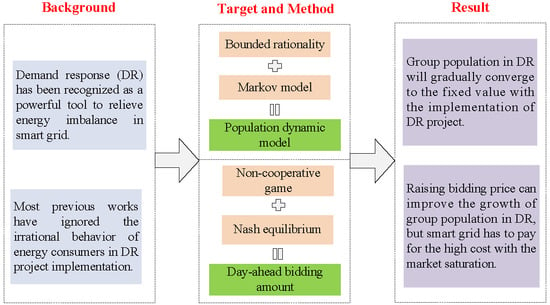For example, Reference [22] proposed a novel non-cooperative game among customers with prospect theory to incorporate the impact of customer irrational behavior, and Reference [23] put forward a dynamic pricing mechanism based on game theory, considering the existence of inexperienced or irrational users. Different from the existing research, this paper mainly concentrates on the analysis of irrational human behavior for residential users in the decision-making process of DR. In our proposed framework, a residential community is responsible for the load aggregation of internal users, and the DR project is divided into multiple stages. The residential community can independently decide whether it will participate in each stage of the DR project. In order to describe the irrationality of communities in the decision on whether to be in DR, a novel decision-making behavior model in each stage of the DR project is proposed based on the Markov chain. Accordingly, the population evolution result of being in DR can be obtained with the implementation of the DR project. Such an evolutionary process of the population is very significant for the grid to measure the feasibility of the designed DR mechanism. Furthermore, in each stage of the DR project, residential communities who are willing to be in DR have to participate in the day-ahead DR market to determine the bidding amount. To reduce the risk of participants’ unreasonable bidding amount and price, a non-cooperative game approach is proposed to describe the competition behavior among communities in the day-ahead DR market. In brief, the contributions of this paper are as follows:

(1) A scenario is proposed for the multi-stage DR project to analyze the population evolution participating in DR considering the residential community’s irrational behavior in the decision-making process, which can provide decision guidance in the design of the DR mechanism for dispatching the center of the smart grid.

(2) A novel decision-making behavior model is formulated with the Markov chain to forecast whether the residential community will participate in DR, which can provide a better understanding of the practical performance of the DR project.

(3) A non-cooperative game approach is formulated to search the bidding equilibrium among residential communities willing to participate in DR, which can contribute to the stability of the DR bidding market.

The rest of this paper is organized as follows. The system model is introduced in Section 2. In Section 3, we formulate the non-cooperative game approach and prove the existence of the Nash equilibrium. And then, the Markov model for the population evolution is given in Section 4. The case study and simulation results are presented in Section 5. Finally, this paper is concluded in Section 6.

2. System Model

A DR framework for residential community is proposed in Figure 1. Assume that there are total I residential communities with the set I = N ∪ M, in which group N contains N residential communities who are willing to participate in DR, while group M contains M communities who are unwilling to participate. Each community contains many residential users with a rich flexible load, such as air condition and an electrical vehicle. The dispatching center of the smart grid is mainly responsible for DR transaction with the residential communities in group N [24,25]. In the day-ahead DR market, since only the bidding price and amount are exchanged between the dispatching center and community, each community does not reveal the details about the energy consumption of native users’ appliances. Therefore, privacy can be protected from the residential community level [26]. Furthermore, the members in each group do not always remain unchanged. After a period of time, each community obtains the opportunity to choose to participate in DR or not. In the paper, such a time slot is set to one week. Since the residential community in the scenario has bounded rationality, we assume that a community can be infected with probability β by each neighboring community in group N, while a community in group N will transfer to group M with probability α. That is, at the beginning of each week, each community will make a new choice with the corresponding probability. Accordingly, in the proposed framework, there exists two time scales: one is a short-time scale for daily energy consumption scheduling with the set T = [1, 2, ..., T]; the other is long-time scale for residential community decision-making with the set H = [1, 2, ..., H].

2.1. Energy Dispatching Model

Assume that residential community n ∈ N chooses to participate in DR in week h ∈ H, then its bidding amount is $L_n^{h,t}$ in time slot t ∈ T. Considering the limitation of flexible DR resources on the residential side, the bidding amount has to satisfy the following constraint:

$$L_n^{h,\min }\le L_n^{h,t}\le L_n^{h,\max }$$

(1)

where $L_n^{h,\min }$ and $L_n^{h,\max }$ represent the minimal and maximal bidding amount of community n in week h, respectively. Therefore, the individual feasible bidding amount set of community n in week h can be expressed as follows:

$${ℒ}_n^h=\left\{{\mathit{L}}_n^h:L_n^{h,\min }\le L_n^{h,t}\le L_n^{h,\max },\forall t\in \mathit{T}\right\}$$

(2)

where ${\mathit{L}}_n^h=\left[L_n^{h,1},L_n^{h,2},\cdots ,L_n^{h,T}\right]$ is the bidding amount set of community n in all dispatching slots. Accordingly, the feasible bidding amount set of all residential communities in group N can be expressed as follows:

$${ℒ}^h={ℒ}_1^h\times {ℒ}_2^h\times \cdots \times {ℒ}_N^h$$

(3)

Note that this paper mainly concentrates on peak load shaving, hence, bidding amount refers to the dispatching amount that will be cut down in real time.

2.2. Bidding Price Model

When a residential community agrees to be scheduled by the dispatching center of the smart grid, it can obtain an economic benefit from the grid, but it firstly has to take part in the day-ahead bidding market. In order to maintain bidding market stability, it is necessary for the dispatching center to design a reasonable bidding price model. In the paper, we assume that the bidding price mechanism must satisfy the following conditions:

(1)

The bidding price model should be smooth or at least piecewise smooth.

(2)

The bidding price in a certain time slot should be a decreasing model with respect to the total bidding amount of all communities in group N.

Accordingly, a linear function is employed as the bidding price model. Since the bidding amount of community n in week h is $L_n^{h,t}$, the total bidding amount of all communities in time slot t can be expressed as:

$$L_h^t={\displaystyle \sum _{n=1}^N{L}_n^{h,t}}$$

(4)

Therefore, the bidding price in the market can be expressed as follows:

$$p_h^t=a_h^t{L}_h^t+b_h^t$$

(5)

where $a_h^t<0$ and $b_h^t>0$ are constants correlated with time slot t and week h. Parameter $a_h^t<0$ can guarantee the bidding price decreases with the increase of the bidding amount and, at the same time, can also effectively reduce the implementation cost of the DR project for the dispatching center.

2.3. Utility Model of Energy Consumption

A residential community receives utility when it consumes energy in its own ways. When the energy consumption of the community is scheduled by the dispatching center of the smart grid, consumption utility will be affected. In order to quantitatively measure the utility, a utility model needs to be formulated. In many DR studies [27,28], quadratic and logarithmic utility functions are frequently used, because they are non-decreasing and their marginal benefits are non-decreasing. In this paper, without loss of generality, the quadratic function is adopted as the utility model. That is:

$$u_n^{h,t}=c_h^t{\left(L_n^{h,t}\right)}^2+d_h^t{L}_n^{h,t}$$

(6)

where $c_h^t>0$ and $d_h^t>0$ are time-varying parameters. Utility Equation (6) shows that, when a residential community shaves $L_n^{h,t}$ energy, then the utility will lose $u_n^{h,t}$. Therefore, the whole utility of community n in all time slots T can be calculated as:

$$u_n^h={\displaystyle \sum _{t=1}^T{u}_n^{h,t}}$$

(7)

Utility Equation (7) shows that community n will lose utility $u_n^h$ when it shaves ${\displaystyle \sum _{t=1}^T{L}_n^{h,t}}$ energy in the daily dispatching period.

3. Non-Cooperative Game for Group N Participating in Day-Ahead Bidding

In this section, we focus on the model formulation for residential communities who participate in DR. According to Figure 1, all communities in group N have to take part in the day-ahead bidding market. Generally, the game-theoretic approach can be divided into a cooperative game and non-cooperative game [18,29]. In this paper, we assume that each community is only concerned about self-interest, and the non-cooperative game approach is employed to optimize communities’ bidding strategy.

3.1. Day-Ahead Bidding Optimization Problem

Load aggregators taking part in DR usually have different optimization targets, such as energy cost or load factor [30]. In the proposed scenario, the main purpose of residential community participating in DR is to obtain extra economic profit. Considering energy consumption scheduling affects residents’ satisfaction, the dispatching center will give corresponding economic compensation to communities in group N. Based on the bidding price Equation (5), economic compensation of community n in all time slots T can be calculated as:

$$e_n^h={\displaystyle \sum _{t=1}^T{p}_h^t{L}_n^{h,t}}={\displaystyle \sum _{t=1}^T\left(a_h^t{L}_h^t+b_h^t\right)L_n^{h,t}}$$

(8)

Since a community’s utility will be reduced in DR participation, each community will take the maximization of the comprehensive income as the target to compete with other communities in the bidding market. That is:

$$\begin{array}{l}\mathrm{maximize}{e}_n^h\left(L_n^{h,t}\right)-u_n^h\left(L_n^{h,t}\right)\\ s.t. L_n^{h,\min }\le L_n^{h,t}\le L_n^{h,\max }\end{array}$$

(9)

Each community will obtain the optimal bidding strategy in each time slot t ∈ T by solving the optimization Equation (9).

3.2. Non-Cooperative Game Formulation

The bidding price in the market is determined by the total bidding amount of all communities in group N. Therefore, the economic compensation of community n is determined not only by its own bidding strategy, but also the bidding strategies of other communities in group N. That is, community n has to take other communities’ strategies into consideration when it makes its bidding strategy. Hence, the bidding strategy problem for residential communities belongs to the typical non-cooperative game. Based on the objective Equation (9), the non-cooperative game can be formulated as follows [31]:

• Players: all residential communities in group N;
• Strategies: the bidding amount $L_n^{h,t}$;
• Payoffs: comprehensive income of community n:

$$R_n^h\left({\mathit{L}}_n^h,{\mathit{L}}_{-n}^h\right)={\displaystyle \sum _{t=1}^T\left[\left(a_h^t-c_h^t\right)L_n^{h,t}+\left(b_h^t-d_h^t\right)+a_h^t{L}_{-n}^{h,t}\right]L_n^{h,t}}$$

(10)

where ${\mathit{L}}_{-n}^h=\left[{\mathit{L}}_1^h,\cdots ,{\mathit{L}}_{n-1}^h,{\mathit{L}}_{n+1}^h,\cdots ,{\mathit{L}}_N^h\right]$ represents the bidding strategy set of other communities except n in group N; $L_{-n}^{h,t}$ represents the total bidding amount of N − 1 communities with:

$$L_{-n}^{h,t}={\displaystyle \sum _{i=1,i\ne n}^N{L}_i^{h,t}}$$

(11)

All residential communities will constantly update their own strategy for the higher economic compensation based on payoff Equation (10). Once all communities in group N obtain their own maximal profit, no one will change the strategy. Such an equilibrium state is called the Nash equilibrium, which can be expressed as:

$$R_n^h({\mathit{L}}_n^{h*},{\mathit{L}}_{-n}^{h*})\ge R_n^h({\mathit{L}}_n^h,{\mathit{L}}_{-n}^{h*})$$

(12)

where $\left({{\mathit{L}}_n^h}^{*},{\mathit{L}}_{-n}^{h*}\right)$ represents the Nash equilibrium of a formulated non-cooperative game.

3.3. Nash Equilibrium

According to the above definition of the Nash equilibrium, this section focuses on the mathematical proof of the existence and uniqueness of the Nash equilibrium.

Lemma 1.

For each residential community n ∈ N, the function $R_n^h\left({\mathit{L}}_n^h,{\mathit{L}}_{-n}^h\right)$ is continuously differentiable in ${\mathit{L}}_n^h$. For the fixed value of ${\mathit{L}}_{-n}^{h,t}$, the function $R_n^h\left({\mathit{L}}_n^h,{\mathit{L}}_{-n}^h\right)$ is concave about ${\mathit{L}}_n^h$.

Proof. 

It is obvious that, $R_n^h\left({\mathit{L}}_n^h,{\mathit{L}}_{-n}^h\right)$ is continuously differentiable in ${\mathit{L}}_n^h$. As for the concavity of $R_n^h\left({\mathit{L}}_n^h,{\mathit{L}}_{-n}^h\right)$, we just need to prove the Hessian matrix of $R_n\left({\mathit{L}}_n,{\mathit{L}}_{-n}\right)$ is negative definite. The Hessian matrix of $R_n^h\left({\mathit{L}}_n^h,{\mathit{L}}_{-n}^h\right)$ is:

$${\nabla }_{L_n^h}^2{R}_n^h\left({\mathit{L}}_n^h,{\mathit{L}}_{-n}^h\right)=\mathrm{diag}{\left[2\left(a_h^t-c_h^t\right)\right]}_{t=1}^T$$

(13)

Due to the negative value of $2\left(a_h^t-c_h^t\right)$, Equation (13) is a diagonal matrix with all diagonal elements being negative. Hence, the Hessian matrix of $R_n^h\left({\mathit{L}}_n^h,{\mathit{L}}_{-n}^h\right)$ is negative definite. Consequently, function $R_n^h\left({\mathit{L}}_n^h,{\mathit{L}}_{-n}^h\right)$ is concave about ${\mathit{L}}_n^h$. □

Definition 1.

The variational inequality (VI), denoted by $\mathrm{VI}\left(ℒ,\mathit{F}\right)$, is to find a vector ${\mathit{x}}^{*}\in ℒ$ such that:

$${\left(\mathit{x}-{\mathit{x}}^{*}\right)}^T\mathit{F}\left({\mathit{x}}^{*}\right)\le 0\hspace{1em}\forall \mathit{x}\in ℒ$$

(14)

According to Lemma 1 and Definition 1, we can obtain the following lemma:

Lemma 2.

The optimization problem of the non-cooperative model (10) is equivalent to the VI problem $\mathrm{VI}\left(ℒ,\mathit{F}\right)$ where:

$$\mathit{F}\left({\mathit{L}}^h\right)={\left[{\mathit{F}}_n\left({\mathit{L}}_n^h,{\mathit{L}}_{-n}^h\right)\right]}_{n=1}^N$$

(15)

where ${\mathit{L}}^h=\left({\mathit{L}}_n^h,{\mathit{L}}_{-n}^h\right)$ and ${\mathit{F}}_n^h\left({\mathit{L}}_n^h,{\mathit{L}}_{-n}^h\right)$ are expressed as follows:

$${\mathit{F}}_n^h\left({\mathit{L}}_n^h,{\mathit{L}}_{-n}^h\right)={\nabla }_{{\mathit{L}}_n^h}{R}_n^h\left({\mathit{L}}_n^h,{\mathit{L}}_{-n}^h\right)$$

(16)

Proof. 

The proof can be found in [32]. □

Based on Lemma 2, the following proposition can be obtained.

Proposition 1.

In the formulated non-cooperative model (10), its Nash equilibrium is unique.

Proof. 

According to Lemma 2, VI problem $\mathrm{VI}\left(ℒ,\mathit{F}\right)$ has the same solution with the solution of Equation (10). That is, we just need to prove the uniqueness of $\mathrm{VI}\left(ℒ,\mathit{F}\right)$’s solution, then Proposition 1 can be proved. According to [33], we know that $\mathrm{VI}\left(ℒ,\mathit{F}\right)$ will have a unique solution when $\mathit{F}\left({\mathit{L}}^h\right)$ is strictly monotone about feasible set $ℒ$.

To prove the strict monotone of $\mathit{F}\left({\mathit{L}}^h\right)$ is to prove:

$${\displaystyle \sum _{t=1}^T{\displaystyle \sum _{n=1}^N\left[\left(x_n^{h,t}-y_n^{h,t}\right)\left({\nabla }_{x_n^{h,t}}{R}_n^h\left({\mathit{x}}^h\right)-{\nabla }_{y_n^{h,t}}{R}_n^h\left({\mathit{y}}^h\right)\right)\right]}}>0$$

(17)

where ${\mathit{x}}^h={\left\{{\mathit{x}}_n^h\right\}}_{n=1}^N\in {ℒ}^h$,${\mathit{y}}^h={\left\{{\mathit{y}}_n^h\right\}}_{n=1}^N\in {ℒ}^h$.

Let ${\mathit{l}}^{h,t}=\left\{x_1^{h,t},x_2^{h,t},\cdots ,x_N^{h,t}\right\}$ and ${\mathit{j}}^{h,t}=\left\{y_1^{h,t},y_2^{h,t},\cdots ,y_N^{h,t}\right\}$, then Equation (17) can be rewritten as follows:

$${\displaystyle \sum _{t=1}^T\left[\left({\mathit{l}}^{h,t}-{\mathit{j}}^{h,t}\right)\left({\nabla }_{{\mathit{l}}^{h,t}}{R}_n^{h,t}\left({\mathit{l}}^{h,t}\right)-{\nabla }_{{\mathit{j}}^{h,t}}{R}_n^{h,t}\left({\mathit{j}}^{h,t}\right)\right)\right]}>0$$

(18)

where:

$$R_n^{h,t}\left({\mathit{l}}^{h,t}\right)=p_h^t{x}_n^{h,t}-u_n^{h,t}$$

and:

$${\nabla }_{{\mathit{l}}^{h,t}}{R}_n^{h,t}\left({\mathit{l}}^{h,t}\right)={\left[{\nabla }_{x_1^{h,t}}{R}_n^{h,t}\left({\mathit{l}}^{h,t}\right),{\nabla }_{x_2^{h,t}}{R}_n^{h,t}\left({\mathit{l}}^{h,t}\right),\cdots {\nabla }_{x_N^{h,t}}{R}_n^{h,t}\left(l^{h,t}\right)\right]}^T$$

If the following condition is satisfied, then Equation (18) will hold:

$$\left({\mathit{l}}^{h,t}-{\mathit{j}}^{h,t}\right)\left({\mathit{g}}_{h,t}\left({\mathit{l}}^{h,t}\right)-{\mathit{g}}_{h,t}\left({\mathit{j}}^{h,t}\right)\right)>0\hspace{1em}\forall t\in \mathit{T}$$

(19)

where ${\mathit{g}}_{h,t}\left({\mathit{l}}^{h,t}\right)={\nabla }_{{\mathit{l}}^{h,t}}{R}_n^{h,t}\left({\mathit{l}}^{h,t}\right)$.

If the Jacobian matrix of ${\mathit{g}}_{h,t}\left({\mathit{l}}^{h,t}\right)$ is negative definite, then Equation (19) will be satisfied. Assume that ${\mathit{G}}_{h,t}\left({\mathit{l}}^{h,t}\right)={\nabla }_{{\mathit{l}}^{h,t}}{\mathit{g}}_{h,t}\left({\mathit{l}}^{h,t}\right)$, then:

$${\mathit{G}}_{h,t}\left({\mathit{l}}^{h,t}\right)+{\mathit{G}}_{h,t}{\left({\mathit{l}}^{h,t}\right)}^T=2\left(a_h^t-c_h^t\right)\left({11}^T+I\right)$$

(20)

where I is a unit matrix and 1 is a N × 1 matrix where all elements are 1. Since characteristic values of 11^T + I are 1 and N + 1, the characteristic values of ${\mathit{G}}_{h,t}\left({\mathit{l}}^{h,t}\right)+{\mathit{G}}_{h,t}{\left({\mathit{l}}^{h,t}\right)}^T$ are $2\left(a_h^t-c_h^t\right)$ and $2\left(N+1\right)\left(a_h^t-c_h^t\right)$. Consequently, ${\mathit{G}}_{h,t}\left({\mathit{l}}^{h,t}\right)+{\mathit{G}}_{h,t}{\left({\mathit{l}}^{h,t}\right)}^T$ is negative definite. That is, $\mathit{F}\left(\mathit{L}\right)$ is a strictly monotone function. Therefore, the Nash equilibrium of the formulated non-cooperative game is unique. □

Based on the above analysis, the Nash equilibrium for the game can be solved. Equation (9) is to search the maximal value of the comprehensive income in all dispatching slots T. But, when the comprehensive income achieves the maximal value in each time slot t ∈ T, then the comprehensive income in all dispatching slots will also achieve the maximal value. That is, Equation (9) can be translated into the following optimization problems:

$$\{\begin{array}{l}\mathrm{maximize}{w}_n^{h,t}=\left[\left(a_h^t-c_h^t\right)L_n^{h,t}+\left(b_h^t-d_h^t\right)+a_h^t{L}_{-n}^{h,t}\right]L_n^{h,t}\\ s.t.\hspace{1em}{L}_n^{h,\min }\le L_n^{h,t}\le L_n^{h,\max }\end{array}\hspace{1em}\forall t\in \mathit{T}$$

(21)

Furthermore, when the bidding strategies of other communities ${\mathit{L}}_{-n}^{h,t}$ are regarded as fixed values, then the optimal bidding strategy of community n can be expressed as follows:

$${\phi }_n\left({\mathit{L}}_{-n}^{h,t}\right)=\arg \underset{L_n^{h,t}}{\mathrm{maximize}}{w}_n^{h,t}\left(L_n^{h,t},{\mathit{L}}_{-n}^{h,t}\right)\hspace{1em}\forall n\in \mathit{N}$$

(22)

where ${\phi }_n\left({\mathit{L}}_{-n}^{h,t}\right)$ represents the optimal bidding strategy of community n corresponding to strategies ${\mathit{L}}_{-n}^{h,t}$; ${\mathit{L}}_{-n}^{h,t}=\left[{\mathit{L}}_1^{h,t},\cdots ,{\mathit{L}}_{n-1}^{h,t},{\mathit{L}}_{n+1}^{h,t},\cdots ,{\mathit{L}}_N^{h,t}\right]$ represents the bidding strategies of other communities in time slot t.

4. Evolution Analysis between Groups N and M

According to the above analysis, the economic compensation of each residential community in group N is correlated not only with the bidding price parameters, but also with the total bidding amount in the market. Therefore, a community’s economic compensation will be influenced when the population of group N changes. In the initial period of the DR project, communities will obtain high economic compensation for participating in DR. Hence, the neighboring communities may be infected to participate in DR for the high economic compensation. However, when the population of group N has consistent growth, the economic compensation of each community will be reduced gradually. Consequently, those residential communities who care more about energy consumption satisfaction will not choose to participate in DR anymore. Finally, the population of group N and group M will reach a dynamic balance. In this section, communities’ transition probability model between group N and group M is formulated, and then the group population is analyzed.

4.1. Transition Probability Model

To describe the population evolution briefly, we define the state of residential community i ∈ I at week h as S_i(h), in which S_i(h) = 0 represents community i belonging to group M is unwilling to participate in DR, S_i(h) = 1 represents community i belonging to group N adopts the DR project. Then, the transition probability can be calculated following four cases.

(1) Case 1: S_i(h) = 0 → S_i(h + 1) = 1

When the state of community i is S_i(h) = 0 at week h, then it may participate in DR if some of its neighboring communities have adopted it. That is, community i can be infected by each neighboring community with probability β, where 0 ≤ β ≤ 1. Such probability shows the effect of social networking or mutual imitation among DR communities. Note that the probability β is a networking-related parameter. Therefore, the greater the number of neighboring communities who participate in DR, the higher the probability community i will adopt the DR project. Consequently, the corresponding transition probability can be expressed as follows:

$$P\left(S_i\left(h+1\right)=1|S_i\left(h\right)=0\right)=1-{\left(1-\beta \right)}^{N_i^h}$$

(23)

where $N_i^h$ is the total number of neighboring communities in group N that have connection to the community i; 1 − β represents the probability that community i is not infected by one neighboring community; ${\left(1-\beta \right)}^{N_i^h}$ represents the probability that community i is not infected by $N_i^h$ neighboring communities.

(2) Case 2: S_i(h) = 0 → S_i(h + 1) = 0

Since community i with S_i(h) = 0 can only choose S_i(h + 1) = 1 or S_i(h + 1) = 0, the probability that community i still remains in group M can be obtained according to Equation (23). That is:

$$P\left(S_i\left(h+1\right)=0|S_i\left(h\right)=0\right)=1-P\left(S_i\left(h+1\right)=1|S_i\left(h\right)=0\right)={\left(1-\beta \right)}^{N_i^h}$$

(24)

(3) Case 3: S_i(h) = 1 → S_i(h + 1) = 0

When the state of community i is S_i(h) = 1 at week h, it may switch back to S_i(h + 1) = 0 at week h + 1. For example, a community may find the DR project is inconvenient or uneconomical and thus abandon it. In this paper, we assume that the probability from S_i(h) = 1 to S_i(h + 1) = 0 are correlated with economic compensation and energy consumption utility. If a community in the group N switches from state 1 to state 0, it will lose economic compensation, but will obtain the corresponding utility. Hence, when economic compensation decreases due to the increasing of group N’s population, the probability from S_i(h) = 1 to S_i(h + 1) = 0 will increase gradually. To quantitatively measure such probability, the average comprehensive income for all communities in group N is defined as:

$${\overline{w}}^h=\frac{1}{N}{\displaystyle \sum _{i\in N}\left(e_i^h-u_i^h\right)}$$

(25)

Basically, the probability from S_i(h) = 1 to S_i(h + 1) = 0 is defined as:

$$\alpha =\eta \left(1-\frac{{\overline{w}}^h}{{\overline{w}}^{h,\max }}\right)$$

(26)

where $\eta$ is a constant parameter; ${\overline{w}}^{h,\max }=\mathrm{maximize}[{\overline{w}}^1,{\overline{w}}^2,\dots ,{\overline{w}}^{\mathrm{h}}]$ represents the maximal value of group N’s average income in the preceding h weeks. Equation (26) shows that the lower income group N receives, the higher probability the community switches from state 1 to state 0. Specifically, when the average income in group N reaches the maximal value, the corresponding probability will reach the minimal value. According to Equations (25) and (26), the transition probability from state 1 to state 0 can be expressed as:

$$P\left(S_i\left(h+1\right)=0|S_i\left(h\right)=1\right)=\alpha =\eta \left(1-\frac{{\overline{w}}^h}{{\overline{w}}^{h,\max }}\right)$$

(27)

(4) Case 4: S_i(h) = 1 → S_i(h + 1) = 1

Similarly, since community i with S_i(h) = 1 can only choose S_i(h + 1) = 1 or S_i(h + 1) = 0, the probability that community i still remains in group N can be obtained according to Equation (27). That is:

$$P\left(S_i\left(h+1\right)=1|S_i\left(h\right)=1\right)=1-P\left(S_i\left(h+1\right)=0|S_i\left(h\right)=1\right)=1-\alpha$$

(28)

In summary, the transition probability model from S_i(h) to S_i(h + 1) can be expressed as follows:

$$P\left(S_i\left(h+1\right)|S_i\left(h\right)\right)=\{\begin{array}{cc}1-{\left(1-\beta \right)}^{N_i^h}& \left(S_i\left(h\right),S_i\left(h+1\right)\right)=\left(0,1\right)\\ {\left(1-\beta \right)}^{N_i^h}& \left(S_i\left(h\right),S_i\left(h+1\right)\right)=\left(0,0\right)\\ \alpha & \left(S_i\left(h\right),S_i\left(h+1\right)\right)=\left(1,0\right)\\ 1-\alpha & \left(S_i\left(h\right),S_i\left(h+1\right)\right)=\left(1,1\right)\end{array}$$

(29)

4.2. Markov Model for Group Population

In reality, the state of a residential community in past weeks has no effect on the decision in future weeks, and the decision result in week h + 1 is only correlated with a community’s state in week h. Therefore, this paper adopts the Markov chain to describe the decision-making process of residential community. The Markov chain mainly indicates that the future decision-making state is independent of the past state and is only dependent on the current state [34]. In our proposed scenario, the Markov chain can be expressed as:

$$P\left(S_i\left(h+1\right)|S_i\left(1\right),\cdots ,S_i\left(h\right)\right)=P\left(S_i\left(h+1\right)|S_i\left(h\right)\right)$$

(30)

where $S_i\left(1\right),\cdots ,S_i\left(h\right)$ are decision-making states from week 1 to week h. Assume that ${\mathrm{Pr}}_N^i\left(h\right)$ and ${\mathrm{Pr}}_M^i\left(h\right)$ are the probabilities of residential community i in group N and group M in week h. Then, the Markov state evolution can be described as:

$$\begin{array}{ll}{\mathrm{Pr}}_N^i\left(h+1\right)& ={\mathrm{Pr}}_N^i\left(h\right)P\left(S_i\left(h+1\right)=1|S_i\left(h\right)=1\right)+{\mathrm{Pr}}_M^i\left(h\right)P\left(S_i\left(h+1\right)=1|S_i\left(h\right)=0\right)\\ & =\left(1-\alpha \right){\mathrm{Pr}}_N^i\left(h\right)+\left(1-{\left(1-\beta \right)}^{N_i^h}\right){\mathrm{Pr}}_M^i\left(h\right)\end{array}$$

(31)

and:

$$\begin{array}{ll}{\mathrm{Pr}}_M^i\left(h+1\right)& ={\mathrm{Pr}}_M^i\left(h\right)P\left(S_i\left(h+1\right)=0|S_i\left(h\right)=0\right)+{\mathrm{Pr}}_N^i\left(h\right)P\left(S_i\left(h+1\right)=0|S_i\left(h\right)=1\right)\\ & ={\left(1-\beta \right)}^{N_i^h}{\mathrm{Pr}}_M^i\left(h\right)+\alpha {\mathrm{Pr}}_N^i\left(h\right)\end{array}$$

(32)

In Equations (31) and (32), ${\left(1-\beta \right)}^{N_i^h}$ can be rewritten as:

$$\begin{array}{ll}{\left(1-\beta \right)}^{N_i^h}& ={\displaystyle {\prod }_{i\in I_i}\left({\mathrm{Pr}}_N^i\left(h\right)\left(1-\beta \right)+{\mathrm{Pr}}_M^i\left(h\right)\right)}={\displaystyle {\prod }_{i\in I_i}\left({\mathrm{Pr}}_N^i\left(h\right)\left(1-\beta \right)+\left(1-{\mathrm{Pr}}_N^i\left(h\right)\right)\right)}\\ & ={\displaystyle {\prod }_{i\in I_i}\left(1-\beta {\mathrm{Pr}}_N^i\left(h\right)\right)}\approx 1-\beta {\displaystyle {\sum }_{i\in I_i}{\mathrm{Pr}}_N^i\left(h\right)}\end{array}$$

(33)

where $I_i$ represents the set of community i’s neighbors in set I. Therefore, Equations (31) and (32) can also be expressed as follows:

$${\mathrm{Pr}}_N^i\left(h+1\right)=\left(1-\alpha \right){\mathrm{Pr}}_N^i\left(h\right)+\left(1-\left(1-\beta {\displaystyle {\sum }_{i\in I_i}{\mathrm{Pr}}_N^i\left(h\right)}\right)\right){\mathrm{Pr}}_M^i\left(h\right)$$

(34)

and:

$${\mathrm{Pr}}_M^i\left(h+1\right)=\left(1-\beta {\displaystyle {\sum }_{i\in I_i}{\mathrm{Pr}}_N^i\left(h\right)}\right){\mathrm{Pr}}_M^i\left(h\right)+\alpha {\mathrm{Pr}}_N^i\left(h\right)$$

(35)

According to the Markov state Equations (34) and (35), the probability for each community i in groups N or M can be calculated. However, the decision of a single community is not our concern and the main purpose in this section is to analyze the group population. For simplification, assume that I residential communities have good communication and each community can be infected by any other I−1 communities. Then, each residential community in I has equal probability to participate in DR. Consequently, we have:

$${\overline{\mathrm{Pr}}}_N={\mathrm{Pr}}_N^i,{\overline{\mathrm{Pr}}}_M={\mathrm{Pr}}_M^i,{\mathit{I}}_i=\mathit{I}$$

(36)

where ${\overline{\mathrm{Pr}}}_N$ and ${\overline{\mathrm{Pr}}}_M$ represent the probability of any community being in group N or M. Then, Equations (34) and (35) are simplified to:

$${\overline{\mathrm{Pr}}}_N\left(h+1\right)=\left(1-\alpha \right){\overline{\mathrm{Pr}}}_N\left(h\right)+\beta I{\overline{\mathrm{Pr}}}_N\left(h\right){\overline{\mathrm{Pr}}}_M\left(h\right)$$

(37)

and:

$${\overline{\mathrm{Pr}}}_M\left(h+1\right)=\left(1-\beta I{\overline{\mathrm{Pr}}}_N\left(h\right)\right){\mathrm{Pr}}_M^i\left(h\right)+\alpha {\overline{\mathrm{Pr}}}_N\left(h\right)$$

(38)

Therefore, the average number of residential communities in groups N and M in week h can be expressed as:

$$\{\begin{array}{c}N\left(h\right)={\overline{\mathrm{Pr}}}_N\left(h\right)I\\ M\left(h\right)={\overline{\mathrm{Pr}}}_M\left(h\right)I\end{array}$$

(39)

According to Equations (37) and (38), the average number of residential communities in groups N and M in week h + 1 can be calculated as:

$$\{\begin{array}{c}N\left(h+1\right)=\left(1-\alpha \right)N\left(h\right)+\beta N\left(h\right)M\left(h\right)\\ M\left(h+1\right)=\left(1-\beta N\left(h\right)\right)M\left(h\right)+\alpha N\left(h\right)\end{array}$$

(40)

Equation (40) is used to describe the population evolution in groups N and M.

4.3. Distributed Algorithm

To search the Nash equilibrium of the formulated non-cooperative game and population evolution result of the residential communities participating in DR, a distributed algorithm is proposed which is shown in Algorithm 1. In the algorithm, an interior point method is employed to solve Equation (22), which has superior performance in solving convex optimization problems. In addition, steps 2–10 are designed to search the Nash equilibrium among communities in the day-ahead bidding market, and steps 11–14 are designed to obtain the population evolution result of residential communities participating in DR.

Algorithm 1: Searching for Nash equilibrium and population evolution result

Input: Parameters $a_h^t$, $b_h^t$, $L_n^{h,\min }$, $L_n^{h,\max }$, etc.

Output: Nash equilibrium, population evolution result.

Initialization: Number of group N in week 1.

1  h = 1; 2   Repeat 3    n = 1;

4     forn ≤ N(h) do

5      Initialize bidding strategy vector ${\mathit{L}}_n^h$;

6      Each community n ∈ N updates ${\mathit{L}}_n^h$ by solving Equation (22); 7      n = n + 1; 8     end 9    Until No community changes its strategy; 10   Return Nash equilibrium $\left({\mathit{L}}_n^{h*},{\mathit{L}}_{-n}^{h*}\right)$; 11  Calculate transition probability α and β; 12  Update group population with Equation (40); 13  h = h + 1; 14  Go back to step 2 until |N(h+1) − N(h)| changes in a termination criterion.

5. Case Study

The performance of the proposed approach is evaluated in this section. In the simulation, assume that there are |I| = 50 residential communities. At the beginning of the DR project (i.e., the 1st week), there are |N| = four residential communities who are willing to participate in DR, and other |M| = 46 communities are in a waiting state. For these communities participating in DR, they have to take part in the day-ahead bidding market to obtain the dispatching amount. Generally, the daily peak hours appear in 10:00–14:00 and 18:00–21:00. Here, energy consumption scheduling during 18:00–21:00 in one day of each week is taken as an example. Accordingly, suppose that peak shaving hours are 18:00–21:00 and a scheduling interval is 15 minutes. That is, residential communities in group N will bid for a load shaving amount in time slots T = [1, 2, ..., 12]. Furthermore, bidding price parameters are shown as (unit: 10³ dollars/MWh): $a_h^t$ = −0.068, $b_h^t$ = 0.553 (t = 1–5 and 11–12); $a_h^t$ = −0.058, $b_h^t$ = 0.774 (t = 6–10). Utility model parameters are shown as (unit: 10^3 dollars/MWh): $c_h^t$ = 0.012, $d_h^t$ = 0.117 (t = 1–5 and 11–12); $c_h^t$ = 0.013, $d_h^t$ = 0.126 (t = 6–10). Transition probability model parameters are shown as: β is in [0.02,0.04], η is in [0.3,0.4]. As for the available DR resource in the community, we assume that the maximal value and minimal value of the DR resource are set as in Figure 2. And each community’s DR resource is given with a random value among the range.

5.1. Evolution Result in Groups N and M

Based on the above simulation parameters, the population evolution result and the Nash equilibrium was obtained by performing Algorithm 1. Note that Algorithm 1 is set to 70 iterations and each iteration means one week. Accordingly, Figure 3 is the convergence process of the population in groups N and M. It depicts that the population in each group gradually converged to the evolutionary equilibrium in 42 weeks. Specifically, in the first 20 weeks, group N’s population increased rapidly from four communities to 36 communities, while between the 21st week and 42nd week, group N’s population increased slowly from 37 communities to 44 communities. Note that, since the average number of communities in a group is deduced from Equation (45), in which the probability ${\overline{\mathrm{Pr}}}_N$ and ${\overline{\mathrm{Pr}}}_M$ are non-integral values, the group’s population in Figure 2 was also a non-integral value. But the group’s population was rounded as an integral value when searching the Nash equilibrium in the day-ahead bidding market.

Figure 4 is the convergence process of the total bidding amount in group N in all dispatching time slots T. From the figure, one can see that, at the beginning of the DR project, the total bidding amount of four communities was only about 20 MWh, while the bidding amount reached 80 MWh after performing the DR project for about 10 weeks. The main reason for such rapid growth was due to the increase of the population in group N. However, the bidding amount tends to reach saturation after 10 weeks. It was because the bidding price was reduced gradually with the further increase of group N’s population and the bidding amount of each community was declined as well. Moreover, the comprehensive income of group N in all dispatching time slots T is shown in Figure 5. It demonstrates that the total income of group N increased firstly and then decreased dramatically in 10 weeks, and finally converged to the fixed value in the weeks after 10 weeks. The reason for such a trend was mainly related with the variation of economic compensation and utility. In the first five weeks, the bidding amount in the market was not very large, then the bidding price was relatively high and the economic compensation increased dramatically with the increase of group N’s population. Therefore, the income in the first five weeks was mainly dependent on the economic compensation. However, with the increase of the bidding amount, the utility that the community lost in DR increased gradually but the economic compensation increased slowly. Therefore, the comprehensive income in the 6th weeks and 10th weeks decreased rapidly. Since the bidding amount tends to be stable after 10 weeks, the total income of group N was also convergent.

From the above evolution result, it is clear that most of the residential communities will be attracted to participate in DR with the implementation of the DR project. However, not all communities in the set I will be involved in DR. When residential communities in the bidding market become saturated, the average economic compensation of each community will be decreased to the minimal value. Consequently, some members in group N will be unwilling to participate in DR and switch from group N to group M with a high probability. At last, the population of groups N and M will reach the dynamic balance.

5.2. Equilibrium Result for Group N

This section shows the Nash equilibrium among the residential communities in group N. In our proposed scenario, at the beginning of each week, the community will choose to participate in DR or not, and then, communities participating in DR have to bid for the dispatching amount in the day-ahead market. Therefore, in each week exists one equilibrium solution and there are altogether 70 equilibrium solutions, considering the DR project was conducted in 70 weeks. For the limitation of paper space, we took the equilibrium solutions of two special weeks (i.e., 1st week and 70th week) as examples to illustrate the optimal bidding strategy.

Figure 6 and Figure 7 are the optimal bidding amounts of each community in the 1st week and 70th week, respectively. In which, communities 1–4 are the communities who were willing to participate in DR at the beginning of the DR project. From the figures, we can see that the bidding amount in the 1st week was much more than that in the 70th week in all 12 time slots. Additionally, the bidding strategies of four communities in each time slot were all different in the 1st week, while four communities had the same bidding strategies in the 70th week. The main reason was that, at the beginning of the DR project, the bidding market needed a large amount of DR resources, hence the community with more DR resources will compete for more dispatching amount. However, when the DR project was conducted for 70 weeks, the DR resource in the market was saturated and the bidding price was also saturated with the lowest value. Consequently, the bidding amount of the community was reduced to the minimal value, even for those communities with abundant DR resources. Actually, in this case study, the bidding amount of each community was only related with bidding price parameters and utility model parameters after the bidding market reached saturation. The bidding amount changed with the change of bidding price parameters. For example, we see that from Figure 7, the values of bidding price parameters were different between t = 1–5 and t = 6–10, then the bidding amount between t = 1–5 and t = 6–10 were also different. Concretely, the average bidding amount of all communities in group N is presented in

Table 1. Average bidding amount of all communities in group N.

Time	Average Bidding Amount (1st Week)	Average Bidding Amount (70th Week)
18:00–18:15	0.256	0.121
18:15–18:30	0.238	0.121
18:30–18:45	0.344	0.121
18:45–19:00	0.371	0.121
19:00–19:15	0.366	0.121
19:15–19:30	0.522	0.203
19:30–19:45	0.692	0.203
19:45–20:00	0.739	0.203
20:00–20:15	0.428	0.203
20:15–20:30	0.543	0.203
20:30–20:45	0.283	0.121
20:45–21:00	0.327	0.121

. From the table, it shows that the maximal bidding amount was 0.739 MWh between 19:45–20:00 in the 1st week, while the maximal bidding amount was only 0.203 MWh between 19:15–20:30 in the 70th week.

In addition, the bidding price in the 1st week and 70th week is shown in Figure 8. It depicts that the bidding price in the 1st week was much higher than the price in 70th week. For example, the highest bidding price in the 1st week was 675 dollars/MWh during 20:00–20:15, while the highest price in the 70th week was only 203 dollars/MWh. Therefore, from the aspect of the dispatching center of the smart grid, the designed bidding price mechanism can effectively reduce the dispatching cost of the grid. Of course, the dispatching center of the smart grid can also control the DR resource amount in the market by regulating price parameters. The next section analyzes the influence of bidding price parameters on DR.

5.3. Impact of Bidding Price Parameters

According to the above analysis, it is clear that bidding price plays an important role in the DR project. It is necessary to analyze how the bidding price affects the DR. Therefore, this section analyzes the influence of bidding price parameters on the population evolution result and the Nash equilibrium. Here, we took initial price parameters (i.e., $a_h^t$ = −0.068, $b_h^t$ = 0.553 (t = 1–5 and 11–12); $a_h^t$ = −0.058, $b_h^t$ = 0.774 (t = 6–10)) as the benchmark, then varied the price parameters by 1.1–2.0 times the benchmark. The corresponding result is presented as follows.

Figure 9 shows the bidding amount of each community and population in group N for different bidding price parameters. Note that the optimal bidding strategy in the figure was the Nash equilibrium in the week that evolution equilibrium was reached. Since the bidding strategies of different communities were all the same under the same price parameters, each community had the same bidding amount in dispatching slots T. From the figure, it depicts that the bidding amount increased gradually with 1.1–2.0 times the benchmark. Specifically, the population in group N increased from 44 to 45 communities when the parameters reached 1.3 times the benchmark. However, the population in group N still had only 45 communities even when price parameters reached 2 times the benchmark. Figure 10 shows the total bidding amount of all communities for different bidding price parameters. It is clear that, although the total bidding amount achieved consistent growth, the increment was declined gradually. By analyzing the above result, it demonstrates that raising the bidding price can improve the growth of the bidding amount, but with the market saturation, the dispatching cost increased for the same increment. Therefore, for the dispatching center of the smart grid, it was very necessary to optimize the bidding price parameters to make a balance between the DR amount and the dispatching cost.

6. Conclusions

This paper not only focused on the evolutionary analysis of group population participating in the DR project, but also the optimization of the bidding strategy in a day-ahead bidding market. In the proposed scenario, a residential community’s irrationality was considered in the decision-making process. In particular, the dynamic evolutionary process of group population was described with the Markov model, and the bidding strategy for communities participating in DR was optimized with the non-cooperative game approach. Furthermore, the uniqueness of the Nash equilibrium was proved with the mathematical method. Finally, a case study was performed to verify the effectiveness of formulated models. It showed that the group population in DR gradually converges to the fixed value with the implementation of the DR project. In addition, by analyzing the influence of bidding price parameters on DR, it showed that raising the bidding price can improve the growth of the group population in DR and the bidding amount, but the smart grid had to pay for the high dispatching cost with market saturation.