Robust Perturbation Observer-based Finite Control Set Model Predictive Current Control for SPMSM Considering Parameter Mismatch

Abstract

In order to improve the dynamics of the surface-mounted permanent magnet synchronous motors (SPMSM) used in servo systems, finite control set model predictive current control (FCS-MPCC) methods have been widely adopted. However, because the FCS-MPCC is a model-based strategy, its performance highly depends on the machine parameters, such as the winding resistance, inductance and flux linkage. Unfortunately, the parameter mismatch problem is common due to the measurement precision and environmental impacts (e.g., temperature). To enhance the robustness of the SPMSM FCS-MPCC systems, this paper proposes a Lundberg perturbation observer that is seldom used in the FCS model predictive control situations to remove the adverse effects caused by resistance and inductance mismatch. Firstly, the system model is established, and the FCS-MPCC mechanism is illustrated. Based on the machine model, the sensitivity of the control algorithm to the parameter mismatch is discussed. Then, the Luenberger perturbation observer that can estimate the general disturbance arising from the parameter uncertainties is developed, and the stability of the observer is analyzed by using the discrete pole assignment technique. Finally, the proposed disturbance observer is incorporated into the FCS-MPCC prediction plant model for real-time compensation. Both simulation and experiments are conducted on a three-phase SPMSM, verifying that the proposed strategy has marked control performance and strong robustness.

1. Introduction

Surface-mounted permanent magnet synchronous motors (SPMSM) that are characterized by high torque density, high efficiency, and a flexible structure have been widely adopted in electric vehicles (EVs), computer numerical control machines, and servo drives [1,2,3]. Usually, excellent control performance (e.g., high dynamic and steady-state characteristics) is highly needed in these applications, placing great demands upon high-performance control strategies [4]. Because of the advantages of fast response and remarkable constraint handling capability, model predictive control (MPC), first proposed in the 1970s, has been developed significantly in the PMSM drives [5,6].

Now, an MPC controller is adopted to achieve varieties of functions, such as flux and power control [7], speed regulation [8], and torque control [9]. In addition, another commonly used application is model predictive current control (MPCC), which contributes to rapid current dynamics [10,11]. There are two typical methods to achieve an MPCC controller, the first of which extends on the traditional vector control method by replacing the proportional integrate (PI) regulator in the current control loop with an MPCC controller but still retaining a modulator for pulse width modulation (PWM) signal generation [12,13]. The other totally eliminates the modulator, directly using the output of the MPCC controller to select the optimal switching states. This method is called finite control set MPCC (FCS-MPCC) [14,15]. Comparatively speaking, because the latter strategy is so easy to understand and implement that it does not require the users to acquire an in-depth knowledge of the optimal control theory [16], FCS-MPCC methods are gaining increasing attention in the industry.

Generally, the implementation of an MPCC controller must include the prediction process, which is based on the machine model, leading to that the system control performance relying highly on the accurate machine parameters, including the winding resistance and inductance and flux linkage. In practice, the PMSM parameter values for MPCC are usually obtained by measurement using meters (except flux linkage, which needs to be tested or observed). However, the parameter (especially the inductance) detection precision varies greatly in terms of different measurement schemes. Even worse, the machine parameters will change in a nonlinear trend when the operating temperature shifts. On these grounds, there will inevitably exist errors between the measured parameters and the real-time values, resulting in current divergence and static errors. Since the control performance of the MPCC approach is sensitive to parameter uncertainties, many scholars are focusing on eliminating the adverse effects caused by the parameter mismatch problems. For example, the adaptive control principle and online parameter identification technology are incorporated into the modulator-based MPCC controllers to suppress the current ripples caused by parameter mismatch [17,18]. By directly observing the motor flux and inductance and then substituting them into the prediction plant, the MPCC algorithm is endowed with high robustness. However, the parameter identification algorithms are usually complex and time-consuming, so when they are executed in each switching frequency, the calculation delay problem gets unexpectedly exacerbated. Papers [19] and [20] use current errors to estimate the real-time flux so as to remove the d-axis current static errors, but integrators have to be adopted, lowering the system bandwidth and dynamics. In addition, another interesting solution to the parameter mismatch issue is to construct the perturbation observers that can be integrated into the prediction plant model [21,22,23]. This method is capable of detecting the general disturbances caused not only by parameter uncertainties but also the system nonlinearities and even external disturbances. Paper [21] proposes a disturbance observer based on feedback compensation to solve the inductance and bus voltage variation problem, and a discrete extended state observer is constructed in [22] to detect the current and disturbances in conditions of parameter variations and improve the robustness of the MPC controller. A discrete Luenberger observer is designed to estimate the future values of stator current and the disturbance for induction machines in [23], but this method has only been used in the modulator-retained MPCC systems, which needs to be deeply investigated in the FCS-MPCC algorithms for PMSM applications.

This paper develops a Luenberger perturbation observer–based FCS-MPCC for SPMSM to improve the robustness against the machine resistance and inductance mismatch that stems from the inaccurate measurement or variations along with the working environment. It is worth mentioning that the disturbance observer is innovatively used for PMSM FCS-MPCC situations. In order to analyze the sensitivity of the FCS-MPCC method to the resistance and inductance variations, the system model in the rotating frame is first established. Then, the relationship between the performance characteristics and parameter errors is theoretically discussed, posing the necessity to employ a disturbance observer for compensation; this is not available in previous studies. Third, a Lundberg observer is designed to obtain the system disturbance, and by the use of pole placement approach, the intrinsic parameters of the observer are designed to guarantee the system stability. Finally, by integrating the estimated disturbance into the prediction model, the robust FCS-MPCC algorithm is achieved. Compared to the traditional FCS-MPCC algorithms, the current divergence and static errors will get suppressed in the resistance and inductance, even flux linkage mismatch situations.

The structure of the rest paper is as follows. Section 2 introduces a system model that is suitable for designing the improved FCS-MPCC algorithms. In Section 3, the impacts of winding resistance and inductance mismatch on the control performance are detailed. Section 4 presents the perturbation observer and the observer-based FCS-MPCC algorithm. Section 5 discusses the simulation and experimental results of the proposed FCS-MPCC algorithms, and Section 6 is the conclusion part.

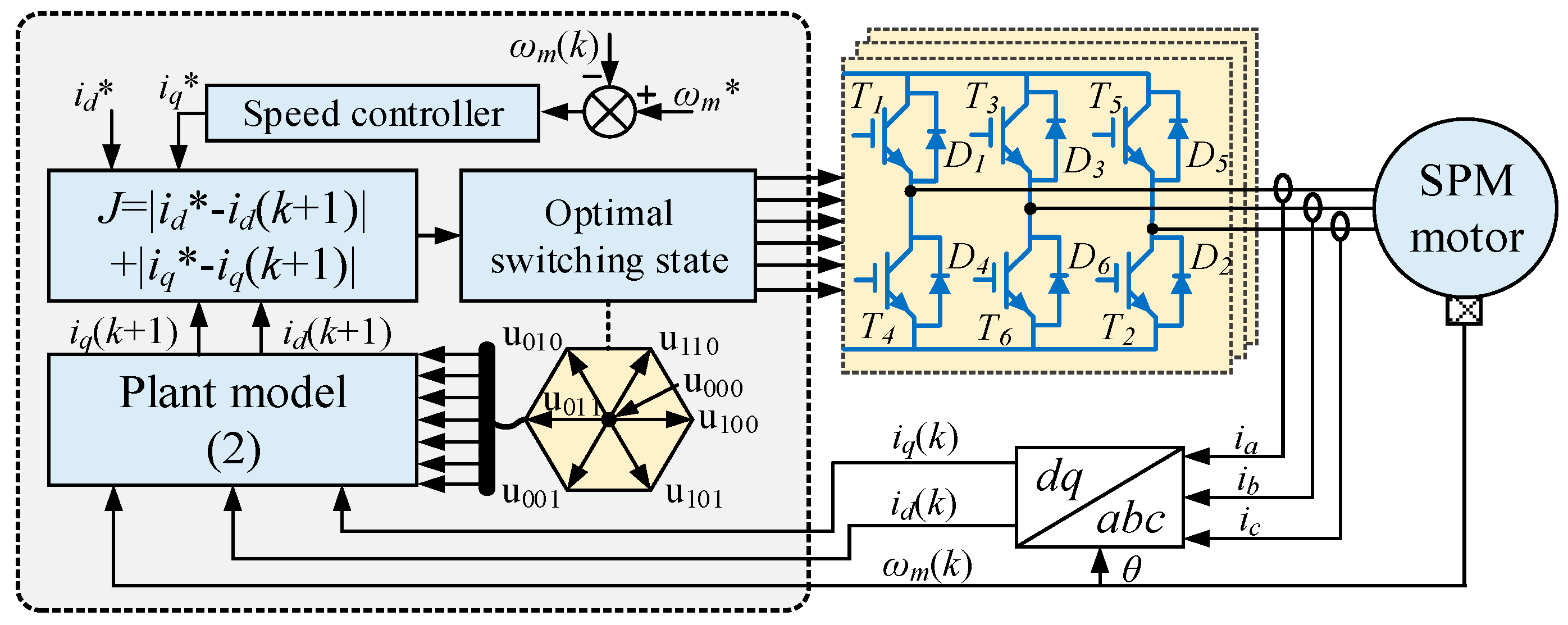
2. Modelling for FCS-MPCC

A state-space model has the advantage that it is explicit and easy to exploit the general behaviors of a multivariable system. In order to estimate the future current states, the electrical dynamics of SPMSMs should be employed for analysis, and the differential equations are as follows, where the iron saturation, eddy current and hysteresis loss are assumed to be negligible:

$$\{\begin{array}{l}\frac{\mathrm{d}{i}_d}{\mathrm{d}t}=-\frac{R_s}{L}{i}_d+p{\omega }_m{i}_q+\frac{u_d}{L}\\ \frac{\mathrm{d}{i}_q}{\mathrm{d}t}=-p{\omega }_m{i}_d-\frac{R_s}{L}{i}_q+\frac{u_q}{L}-\frac{{\mathsf{\Psi }}_f}{L}p{\omega }_m\end{array}$$

(1)

where i_d, i_q are stator dq-axis current and u_d, u_q are dq-axis control voltage. L is the winding inductance, and the stator winding resistance is R_s. ω_m is the rotor mechanical angular speed. Additionally, p represents the number of pole pairs, and ψ_f is the permanent magnet flux linkage. Practically, the continuous machine model must be discretized in a time step of T (switching time) to calculate the future states. When forward Euler discretization is used, the prediction plant model is derived as follows:

$$\{\begin{array}{l}{i}_d(k+1)=\frac{L-T{R}_s}{L}{i}_d(k)+Tp{\omega }_m(k)i_q(k)+\frac{T}{L}{u}_d(k)\\ i_q(k+1)=-Tp{\omega }_m(k)i_d(k)+\frac{L-T{R}_s}{L}{i}_q(k)+\frac{T}{L}{u}_q(k) -\frac{T{\mathsf{\Psi }}_{f}p}{L}{\omega }_m(k)\end{array}$$

(2)

where i_d(k), i_q(k) and ω_m(k) are the measured states at the kth sampling instant. i_d(k + 1) and i_q(k + 1) are the predicting values at the (k + 1)th period.

When an FCS-MPCC algorithm is implemented, the candidate control voltages are directly substituted into the machine model one by one to predict the next-step states. As for a two-level inverter, a total of seven phase voltage vectors that are denoted as v₀₀₀, v₁₀₀, v₁₁₀, v₀₁₀, v₀₁₁, v₀₀₁, and v₁₀₁ are among the alternatives:

$$u_{s_a{s}_b{s}_c}=\left[\begin{array}{l}{u}_a\\ u_b\\ u_c\end{array}\right]=\frac{U_{dc}}{3}\left[\begin{array}{l} 2 1 1\\ -1 2 1\\ -1 1 2\end{array}\right]\left[\begin{array}{l}{s}_a\\ s_b\\ s_c\end{array}\right]$$

(3)

where [s_a, s_b, s_c]^T includes [0, 0, 0]^T, [1, 0, 0]^T, [1, 1, 0]^T, [0, 1, 0]^T, [0, 1, 1]^T, [0, 0, 1]^T, and [1, 0, 1]^T, and they are the switching states. U_dc is the DC source voltage. [u_a, u_b, u_c]^T are the terminal phase voltages. By the use of abc/dq transformation, the control voltage sets used for prediction can be expressed as

$$\left[\begin{array}{l}{u}_d(k)\\ u_q(k)\end{array}\right]=\sqrt{\frac{2}{3}}\left[\begin{array}{l} \cos \theta \frac{ \sqrt{3}\sin \theta -\cos \theta }{2} \frac{ -\sqrt{3}\sin \theta -\cos \theta }{2}\\ -\sin \theta \frac{ \sin \theta +\sqrt{3}\cos \theta }{2} \frac{ \sin \theta -\sqrt{3}\cos \theta }{2}\end{array}\right]\cdot u_{s_a{s}_b{s}_c}$$

(4)

where θ is the rotor position.

The block diagram of the FCS-MPCC implementation is shown in Figure 1. Taking the kth period as an example, the mechanism of the method can be divided into the following four stages:

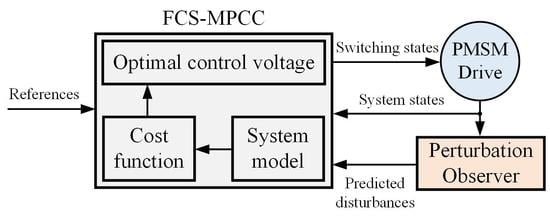
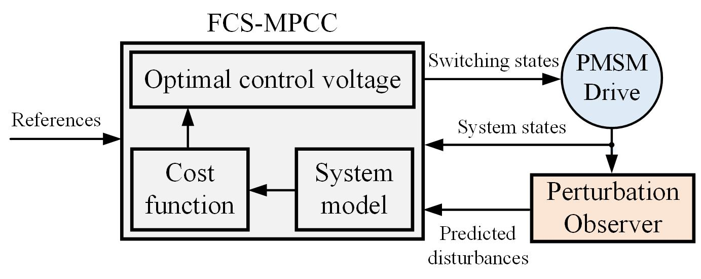
• Measurement and abc/dq transformation: the current and position sensors are used to measure the phase currents (i_a, i_b and i_c), rotor position (θ) and speed ω_m(k). Then, the measured currents are transformed to the dq-axis currents (i_d(k) and i_q(k)) according to the real-time rotor position.
• Prediction: use i_d (k), i_q (k) and ω_m(k) to estimate the future current states i_d (k + 1) and i_q (k + 1) for all the seven candidate voltage vectors.
• Evaluation: substitute the seven the predicted values into the cost function (5) and determine the optimal voltage vector that minimizes the value of J.

  $$J=|i_d{}^{*}-i_d(k+1)|+|i_q{}^{*}-i_q(k+1)|$$

  (5)

  where i_d^* and i_q^* are the reference d- and q-axis currents, respectively.
• Switching state application: apply the corresponding optimum switching state to the drive system.

3. Impacts of Parameter Mismatch on FCS-MPCC Properties

This section will theoretically analyze the impacts of winding resistance and inductance disturbance on the control performance of the FCS-MPCC strategy. Under the verification of the simulation, a crucial conclusion that the parameter disturbance needs to be compensated by the use of perturbation observers can be drawn.

3.1. Analysis on Stability

Assuming that the real winding resistance and inductance of the machine are R_s and L, respectively, the future states can be calculated directly by model (2). The measured resistance and inductance used for FCS-MPCC controller are denoted as R_s0 and L₀, and the predicted d, q-axis currents are i_d0 (k + 1) and i_q0 (k + 1), respectively. The prediction plant can be rewritten as

$$\{\begin{array}{l}{i}_{d0}(k+1)=\frac{L_0-T{R}_{s0}}{L_0}{i}_d(k)+Tp{\omega }_m(k)i_q(k)+\frac{T}{L_0}{u}_d(k)\\ i_{q0}(k+1)=-Tp{\omega }_m(k)i_d(k)+\frac{L_0-T{R}_{s0}}{L_0}{i}_q(k)+\frac{T}{L_0}{u}_q(k) -\frac{T{\mathsf{\Psi }}_{f}p}{L_0}{\omega }_m(k)\end{array}$$

(6)

It can be noticed that the control voltages in Equation (2) equal those in Equation (6), so it can be further derived that

$$\{\begin{array}{l}{i}_d(k+1)=\frac{L_0}{L}{i}_{d0}(k+1)+\frac{\Delta L-T\Delta R_s}{L}{i}_d(k)+\frac{\Delta L}{L}Tp{\omega }_m(k)i_q(k)\\ i_q(k+1)=\frac{L_0}{L}{i}_{q0}(k+1)+\frac{\Delta L-T\Delta R_s}{L}{i}_q(k)-\frac{\Delta L}{L}Tp{\omega }_m(k)i_d(k)\end{array}$$

(7)

where ∆R_s = R_s − R_s0, ∆L = L − L₀, and they represent the deviation magnitude between the real machine parameters and the measured values.

Generally, the sampling time T is very short, so the influence of it can be ignored. Take the z-transformation of (7), the discrete transfer function from i_d0,_q0 to i_d,_q can be derived as

$$G(z)=\frac{i_{d,q}(z)}{i_{d,q0}(z)}=\frac{L_0}{Lz+(L_0-L)}$$

(8)

It can be seen that the pole of the system is $z=1-\frac{L_0}{L}$. According to the stability criterion, the magnitude of the pole should less than 1, that is, |z| < 1. Therefore, the condition that stabilizes a model-based FCS-MPCC controller should be

$$0<L_0<2L$$

(9)

According to Equation (9), when the measured inductance that is substituted into the plant model for prediction is less than twice the real values, the system will remain stable. However, as the inductance deviation enlarges, the stability of the system will degrade, and the larger the deviation is, the more seriously the system oscillates. Moreover, due to the sampling time effect, the resistance disturbance scarcely influences the stability of the FCS-MPCC controller. In order to verify the theoretical results, a simulation is carried out on a three-phase SPMSM whose real parameters are shown in

Table 1. Surface-mounted permanent magnet synchronous motor (SPMSM) parameters.

Variable	Description	Value	Unit
Udc	DC-link voltage	310	V
L	real inductance	2.4	mH
Rs	real resistance	0.175	Ω
T	sampling time	0.1	ms
p	number of pole pairs	3	-
ωrated	rated speed	520	rad/s
Trated	rated torque	5	Nm
Ψf	PM flux	0.075	Wb

.

Figure 2 illustrates the current control performance when different measured inductance values are adopted for the traditional SPMSM FCS-MPCC algorithm. At first, the machine speeds up from standstill to 520 rad/s, and the speed levels off until 2 s. At 1 s, the rated load is imposed on the rotor shaft. When the inductance used for prediction equals the real value, the q-axis reference current generated by the speed controller is zero under no-load condition and 15.3 A with rated load imposed (as in Figure 2a). Besides, the currents can be controlled to track the given position with low ripples. For example, the d-axis current ripples are within ±1.8 A under the load condition. These mean that there are no static errors and the system is of high stability. Figure 2b shows that when L₀ is set as 2L (∆L = L), even though the q-axis reference current is still zero under no load, it witnesses a slight increase to 15.6 A under load compared to Figure 2a. More importantly, the current ripples grow to (+3, −2) A, representing that the stability of the system decreases. When the inductance used for prediction increases to 5L, the q-axis reference current cannot level off at zero but fluctuates around 7 A, and meanwhile, it fluctuates around 21.3 A under load (as in Figure 2c). In this case, although the system still works, the current cannot keep stable any longer, which can be regarded to indicate that the system FCS-MPCC controller is not convergent. As for the d-axis current, the current ripples have increased to (+20, −10) A. By contrast, when assuming that the measured inductance decreases to 0.5L, the q-axis reference current does not show fluctuations, and the current ripples are still small, although a static error appears (as in Figure 2d). The results illustrate that the theoretical analysis on the system stability is effective.

3.2. Analysis on Steady-State Performance

Figure 2 indicates that the parameter mismatch can not only lead to the reduction of an FCS-MPCC based system stability but also the increase of the steady-state errors. Although paper [24] discusses the several sources (inductance and flux disturbance, etc.) of the current static errors, it neglects the impact of winding resistance. This part will comprehensively explain the relationship between the static errors and both resistance and inductance.

After the machine reaches the stable operating region, the currents of two adjacent switching periods can be regarded to be the same since the sampling time is very short, namely,

$$\{\begin{array}{l}{i}_d(k+1)=i_d(k)\\ i_q(k+1)=i_q(k)\end{array}$$

(10)

By substituting Equation (10) into Equation (7), the relationship between the real currents and the estimated values can be described as follows:

$$\{\begin{array}{l}\Delta i_d=i_d(k+1)-i_{d0}(k+1)=(-\frac{\Delta R_s}{L_0}{i}_d(k)+\frac{\Delta L}{L_0}p{\omega }_m(k)i_q(k))\cdot T\\ \Delta i_q=i_q(k+1)-i_{q0}(k+1)=(-\frac{\Delta R_s}{L_0}{i}_q(k)-\frac{\Delta L}{L_0}p{\omega }_m(k)i_d(k))\cdot T\end{array}$$

(11)

According to Equation (11), first, the currents’ static errors are proportionally related to the switching period in the stable conditions. Luckily, the switching period is usually small (0.1 ms), so the current static errors can be small unless the parameter disturbances are significant. When the machine works at the rated points and the d-axis current is controlled to remain zero, Equation (11) can be simplified as

$$\{\begin{array}{l}\Delta i_d=\frac{\Delta L}{L_0}Tp{\omega }_{m\_rated}\cdot i_{q\_rated}=\frac{\Delta L}{L-\Delta L}Tp{\omega }_{m\_rated}\cdot i_{q\_rated}\\ \Delta i_q=-\frac{\Delta R_s}{L-\Delta L}T{i}_{q\_rated}\end{array}$$

(12)

where i_{q_rated} and ω_{m_rated} are the rated q-axis current and speed, respectively. In terms of i_d, the static error is closely relevant to inductance mismatch, while the resistance disturbance has little influence. Obviously, the lower the magnitude of ∆L, the smaller the d-axis current static error becomes. That can be verified by the simulation results in Figure 2. Another interesting phenomenon is that once inductance disturbance occurs, the static error is also influenced by the machine speed, and it will reach the peak position when the speed is at the maximum value. As for the q-axis current, the resistance and the inductance deviations have a more complex impact on the static error, which are determined by the magnitude of ∆L and ∆R_s. These represent that parameter mismatch will greatly reduce the steady-state control performance of the FCS-MPCC controller.

For the sake of intuitive analysis, on the condition that the system is stable, that is, |∆L| < L, the simulation results of the current control performance are depicted in Figure 3 when different measured resistance and inductance values are considered. The simulation setup is the same to the above. In Figure 3a,b, the inductance used for prediction equals the real value, but the resistance R_s0 is 0.5R_s and 5R_s, respectively. It can be seen that the static errors nearly stand at zero. This means that the resistance disturbance scarcely influences the steady-state performance, which complies with the theoretical results. Figure 3c,d illustrate the simulation results when the measured inductance equals the half of real value and R_s0 is 0.5R_s and 5R_s, respectively. The d- and q-axis current static errors are 0.7 A and −0.55 A in Figure 3c, while they are 0.5 A and −0.65 A in Figure 3d, which are similar to the errors in Figure 2d. These further prove that the impact of the inductance mismatch on the control performance is more significant than that of the resistance disturbance. As for the cases that ∆L = −L, Figure 3e,f illustrate that the current static errors get larger. In detail, when ∆R_s=0.5R_s, the d- and q-axis current static errors are 0.95 A and −0.9A, and when ∆R_s = 5R_s, the d- and q-axis current static errors are 0.95 A and −1.1 A, respectively.

Overall, if the winding inductance and resistance used in FCS-MPCC controllers do not accurately comply with the real parameters, current static errors will appear, and even worse, the system will become unstable when the parameter deviations are very large. Therefore, it is necessary to introduce a perturbation observer to detect the real-time disturbance caused by the parameter mismatch and compensate the FCS-MPCC algorithms.

4. Luenberger Perturbation Observer–based FCS-MPCC

Luenberger observer is constructed depending on the state equations of a system, and it takes the errors between the measurable and observable states as the feedback. By selecting an appropriate gain, the feedback errors can quickly approach zero so as to ensure that the observed variables constantly move to the accurate states, and the required variables that are hard to detect can finally be obtained. In this section, a stable Luenberger observer is designed to first observe the system disturbances. Then, the estimated disturbances are directly used to compensate the FCS-MPCC controller, enhancing its robustness against the resistance and inductance deviations.

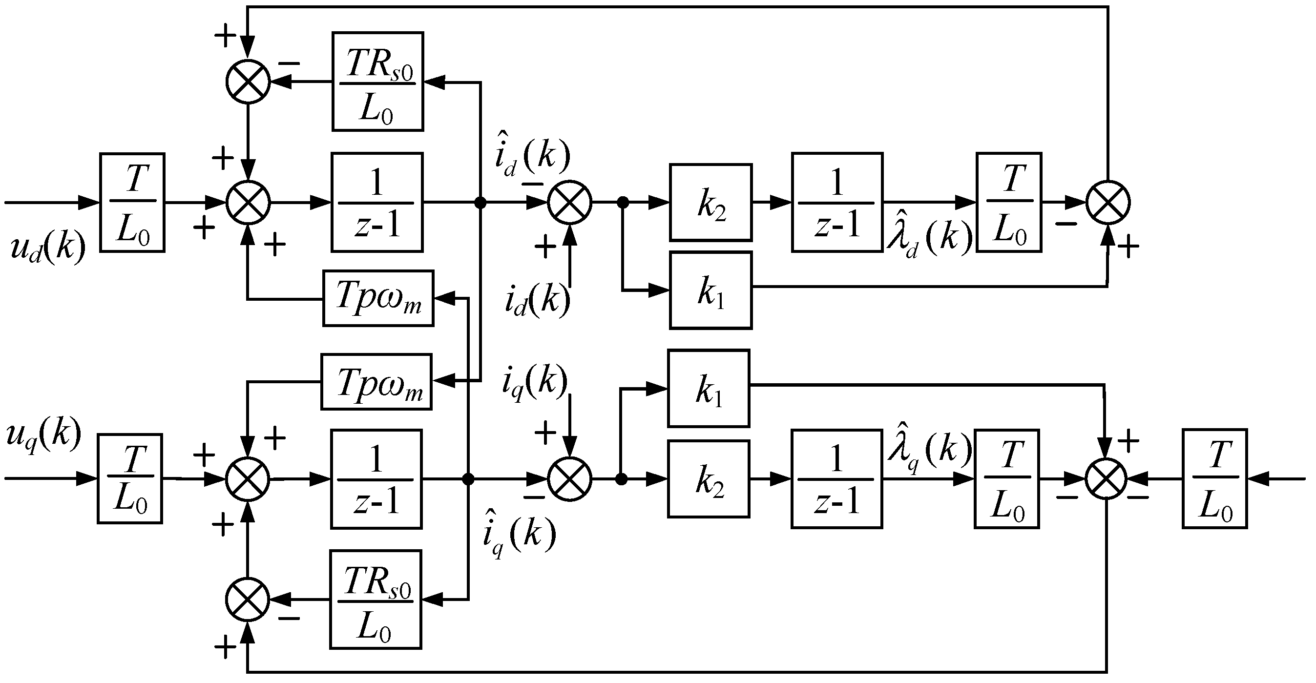
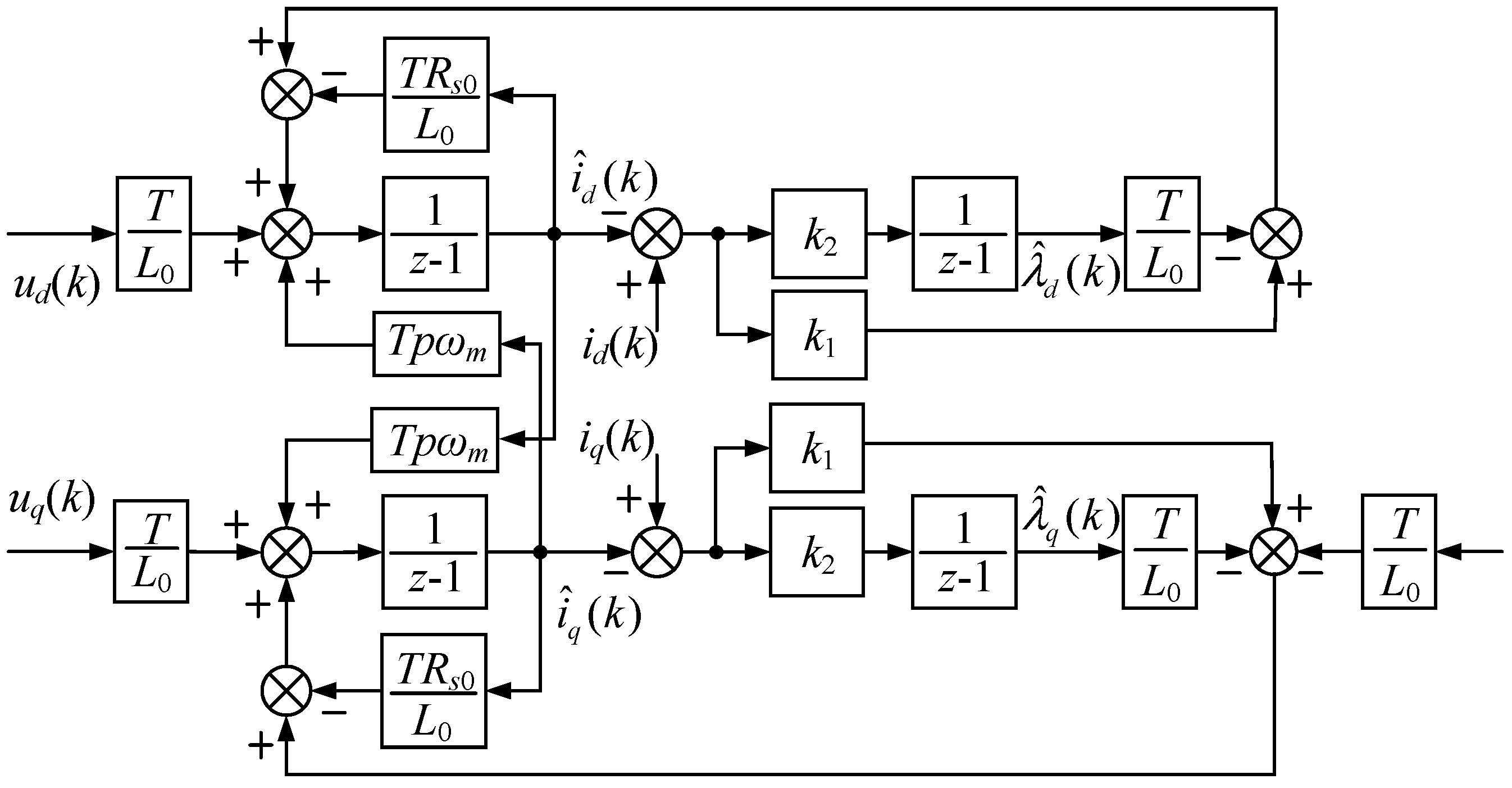
4.1. Design of Luenberger Observer for SPMSM

Taking ∆R_s and ∆L into account, the machine model (1) can be rewritten as

$$\{\begin{array}{l}\frac{\mathrm{d}{i}_d}{\mathrm{d}t}=-\frac{R_{s0}+\Delta R_s}{L_0+\Delta L}{i}_d+p{\omega }_m{i}_q+\frac{u_d}{L_0+\Delta L}\\ \frac{\mathrm{d}{i}_q}{\mathrm{d}t}=-p{\omega }_m{i}_d-\frac{R_{s0}+\Delta R_s}{L_0+\Delta L}{i}_q+\frac{u_q}{L_0+\Delta L}-\frac{{\mathsf{\Psi }}_f}{L_0+\Delta L}p{\omega }_m\end{array}$$

(13)

Obviously, it is difficult to extract the d, q-axis disturbance terms in Equation (13) which can be treated as a current equation. Therefore, expand (13) to a voltage equation as follows:

$$\{\begin{array}{l}{u}_d=(L_0+\Delta L)\frac{\mathrm{d}{i}_d}{\mathrm{d}t}+(R_{s0}+\Delta R_s)i_d-(L_0+\Delta L)p{\omega }_m{i}_q\\ u_q=(L_0+\Delta L)\frac{\mathrm{d}{i}_q}{\mathrm{d}t}+(L_0+\Delta L)p{\omega }_m{i}_d+(R_{s0}+\Delta R_s)i_q+p{\omega }_m{\mathsf{\Psi }}_f\end{array}$$

(14)

Then, the disturbance terms which can be denote as λ_d and λ_q are as follows:

$$\{\begin{array}{l}{\lambda }_d=\Delta L\frac{\mathrm{d}{i}_d}{\mathrm{d}t}+\Delta R_s{i}_d-\Delta Lp{\omega }_m{i}_q\\ {\lambda }_q=\Delta L\frac{\mathrm{d}{i}_q}{\mathrm{d}t}+\Delta Lp{\omega }_m{i}_d+\Delta R_s{i}_q\end{array}$$

(15)

And the SPMSM model containing the disturbances can be derived as

$$\{\begin{array}{l}\frac{\mathrm{d}{i}_d}{\mathrm{d}t}=-\frac{R_{s0}{i}_d}{L_0}+p{\omega }_m{i}_q-\frac{{\lambda }_d}{L_0}+\frac{u_d}{L_0}\\ \frac{\mathrm{d}{i}_q}{\mathrm{d}t}=-p{\omega }_m{i}_d-\frac{R_{s0}{i}_q}{L_0}-\frac{p{\omega }_m{\mathsf{\Psi }}_f}{L_0}-\frac{{\lambda }_q}{L_0}+\frac{u_q}{L_0}\end{array}$$

(16)

Apart from i_d and i_q, set λ_d and λ_q as the state variables, that is, x = [i_d, i_q, λ_d, λ_q]^T. Paper [25] proves that it is appropriate to assume that the change rate of λ_d and λ_q equals zero. On this ground the state equations of the system will get changed to

$$\begin{array}{l}\frac{\mathrm{d}x}{\mathrm{d}t}=Ax+{\rm B}u+D\\ y=Cx\end{array}$$

(17)

where y = [i_d, i_q, i_d, i_q]^T, u [u_d, u_q, 0, 0]^T and $A=\left[\begin{array}{cccc}-\frac{R_{s0}}{L_0}& p{\omega }_m& -\frac{1}{L_0}& 0\\ -p{\omega }_m& -\frac{R_{s0}}{L_0}& 0& -\frac{1}{L_0}\\ 0& 0& 1& 0\\ 0& 0& 0& 1\end{array}\right]$, $B=\left[\begin{array}{cccc}\frac{1}{L_0}& 0& 0& 0\\ 0& \frac{1}{L_0}& 0& 0\\ 0& 0& 0& 0\\ 0& 0& 0& 0\end{array}\right]$, $C=\left[\begin{array}{cccc}1& 0& 0& 0\\ 0& 1& 0& 0\\ 1& 0& 0& 0\\ 0& 1& 0& 0\end{array}\right],$ $D=\left[\begin{array}{c}0\\ -\frac{p{\omega }_m{\mathsf{\Psi }}_f}{L_0}\\ 0\\ 0\end{array}\right]$. According to the standard construction approach of a Luenberger observer [26], the perturbation observer can be described as

$$\begin{array}{l}\frac{\mathrm{d}\widehat{x}}{\mathrm{d}t}=A\widehat{x}+{\rm B}u+D+F(y-\widehat{y})\\ \widehat{y}=C\widehat{x}\end{array}$$

(18)

where $\widehat{x}={[{\widehat{i}}_d, {\widehat{i}}_q,{\widehat{\lambda }}_d,{\widehat{\lambda }}_q]}^{\mathrm{T}}$ and it represents the observed variables, $\widehat{y}={[{\widehat{i}}_d, {\widehat{i}}_q,{\widehat{i}}_d, {\widehat{i}}_q]}^{\mathrm{T}}$ and F is the feedback gain matrix, $F=\left[\begin{array}{cccc}{k}_1& 0& 0& 0\\ 0& k_2& 0& 0\\ 0& 0& k_1& 0\\ 0& 0& 0& k_2\end{array}\right]$. k₁ and k₂ are constants that need to be adjusted to make the observer stable. After applying the Euler discretization to the observer, the discrete disturbance observer turns out to be

$$\widehat{x}(k+1)=E\widehat{x}(k)+T{\rm B}u(k)+TD+TF(y(k)-\widehat{y}(k))$$

(19)

where $E=\left[\begin{array}{cccc}1+\frac{R_{s0}T}{L_0}& -Tp{\omega }_m(k)& -\frac{T}{L_0}& 0\\ -Tp{\omega }_m(k)& 1-\frac{T{R}_{s0}}{L_0}& 0& -\frac{T}{L_0}\\ 0& 0& 1& 0\\ 0& 0& 0& 1\end{array}\right]$. The block diagram of the proposed disturbance observer is shown in Figure 4.

4.2. Stability Analysis of Observer

In order to discuss the stability of the observer, expand Equation (19), and it can be derived that

$$\left[\begin{array}{l}{\widehat{i}}_d(k+1)\\ {\widehat{i}}_q(k+1)\\ {\widehat{\lambda }}_d(k+1)\\ {\widehat{\lambda }}_q(k+1)\end{array}\right]=E^{\prime }\left[\begin{array}{l}{\widehat{i}}_d(k)\\ {\widehat{i}}_q(k)\\ {\widehat{\lambda }}_d(k)\\ {\widehat{\lambda }}_q(k)\end{array}\right]+\left[\begin{array}{l}\frac{T{u}_d(k)}{L_0}\\ \frac{T{u}_q(k)}{L_0}\\ \hspace{0.17em}\hspace{0.17em}\hspace{0.17em}0\\ \hspace{0.17em}\hspace{0.17em}\hspace{0.17em}0\end{array}\right]+\left[\begin{array}{l}{k}_{1}T{i}_d(k)\\ k_{2}T{i}_q(k)\\ k_{1}T{i}_d(k)\\ k_{2}T{i}_q(k)\end{array}\right]$$

(20)

where $E^{\prime }=\left[\begin{array}{cccc}1+\frac{R_{s0}T}{L_0}-k_{1}T& -Tp{\omega }_m(k)& -\frac{T}{L_0}& 0\\ -Tp{\omega }_m(k)& 1-\frac{T{R}_{s0}}{L_0}-k_{2}T& 0& -\frac{T}{L_0}\\ -k_1& 0& 1& 0\\ 0& -k_2& 0& 1\end{array}\right]$. E^’ is the eigenmatrix of the discrete observer model. Only when the eigenvalues of E^’ are all distributed in the unit circle in z-domain will the observer remain stable. Since T is small, an appropriate assumption that $\frac{R_{s0}T}{L_0}=0$ and $Tp{\omega }_m(k)=0$ can be made. Further, the eigenvalues of E^’ can be obtained by solving the following characteristic equation:

$$|\lambda I-E^{\prime }|=-{({\lambda }^2+(k_1-2)\lambda +1-k_1-\frac{T}{L_0}{k}_2)}^2=0$$

(21)

Then, the values of the poles P for the discrete observer are equal to those eigenvalues, namely,

$$P(z)={\lambda }_{1,2}=1-\frac{k_1}{2}\pm \frac{\sqrt{L_0{k}_1{}^2+4k_{2}T}}{2L_0{}^2}$$

(22)

where λ₁ and λ₂ are the solutions of Equation (21). It can be noticed that the poles of the observer are mainly determined by the gains k₁, k₂ and the measured inductance L₀. In the process of control, L₀ is fixed. In order to maintain the observer stable, k₁ and k₂ need to be properly designed. The condition that places the two pole points into the unit circle is that

$$\{\begin{array}{l}0<k_1<4\\ k_2>-\frac{(4+k_1)(L-\Delta L)}{4T}\end{array}$$

(23)

In addition to the system stability, we should consider the dynamic performance of the observer as well. According to the control theory in [27], in order to ensure marked dynamic performance, the pole points should be in the right half of the unit circle. Now, there exist two ways to design the poles: (1) assign two complex poles of which real part is over zero. (2) assign two real poles that are larger than zero. In terms of the first method, the following equations need to be satisfied:

$$\{\begin{array}{l}1-\frac{k_1}{2}>0\\ L_0{k}_1{}^2+4k_{2}T<0\end{array}\to \{\begin{array}{l}{k}_1<2\\ k_2<-\frac{(L-\Delta L)k_1{}^2}{4T}\end{array}$$

(24)

However, because the sign of (L − ∆L) is uncertain, it is impossible to design a fixed k₂ to simultaneously meet the requirements in both Equation (23) and Equation (24).

When the two poles are real, the following equations can be obtained:

$$\{\begin{array}{l}1-\frac{k_1}{2}>0\\ L_0{k}_1{}^2+4k_{2}T\ge 0\end{array}\to \{\begin{array}{l}{k}_1<2\\ k_2\ge -\frac{(L-\Delta L)k_1{}^2}{4T}\end{array}$$

(25)

According to Equation (23) and Equation (25), the values of k₁ and k₂ should satisfy the conditions of

$$\{\begin{array}{l}0<k_1<2\\ k_2>\max (-\frac{(L-\Delta L)k_1{}^2}{4T},-\frac{(4+k_1)(L-\Delta L)}{4T})\end{array}$$

(26)

Thus, k₁ and k₂ can be selected as

$$\{\begin{array}{l}{k}_1=1\\ k_2=\frac{3(4+k_1)}{4T}|L-\Delta L|=\frac{15}{4T}|L-\Delta L|\end{array}$$

(27)

Generally speaking, the motor inductance is not large (0.1 mH–200 mH) [1,2,3,4,6,8,10]. Hence, the realistic error between the real inductance and measured inductance should not exceed 1 H. In this paper, let k₂ equal $\frac{15}{4T}$. Now, both the stability and good dynamics of the observer can be guaranteed.

4.3. Implementation of Luenberger-based FCS-MPCC

After obtaining the disturbances caused by parameter mismatch, they can be used to compensate the prediction plant model used for FCS-MPCC. In this case, the measured parameters are still used for future state calculation, but the improved algorithm becomes more robust. With disturbance compensation, the machine plant model can be described as

$$\{\begin{array}{l}{i}_d(k+1)=\frac{L_0-T{R}_{s0}}{L_0}{i}_d(k)+Tp{\omega }_m(k)i_q(k)+\frac{T}{L_0}{u}_d(k)-\frac{T}{L_0}{\widehat{\lambda }}_d(k)\\ i_q(k+1)=-Tp{\omega }_m(k)i_d(k)+\frac{L_0-T{R}_{s0}}{L_0}{i}_q(k)+\frac{T}{L_0}{u}_q(k) -\frac{T{\mathsf{\Psi }}_{f}p}{L_0}{\omega }_m(k)-\frac{T}{L_0}{\widehat{\lambda }}_q(k)\end{array}$$

(28)

The block diagram of the Luenberger disturbance observer–based FCS-MPCC implementation is illustrated in Figure 5. The implementation procedures are still in accordance with those in Section 2.

5. Simulation and Experimental Results

In this part, simulation and experiments are conducted on a three-phase SPMSM whose parameters are also consistent with Table 1 to verify the effectiveness of the proposed Luenberger observer–based FCS-MPCC strategy working under parameter mismatch situations. The test bench is shown Figure 6. Insulated gate bipolar transistor (IGBT) modules, FP25R12KT3, constitute the voltage inverter with the switching frequency of 10 kHz. The proposed observer algorithm and the FCS-MPCC algorithm are implemented on an RT Lab–based control board. The motor d, q-axis currents are calculated by the digital controller. Another motor driven by an Automation Drive FC 301 with torque control mode is coupled to the test machine, providing the required load torque.

In order to comprehensively verify that the proposed observer is able to compensate different types of disturbances, the following four cases are considered: (1) L₀ = 2L, R_s0 = 0; (2) L₀ = 0, R_s0 = 5R_s; (3) L₀ = 0.5L, R_s0 = 0.5R_s; 4) L₀ = 2L, R_s0 = 5R_s.

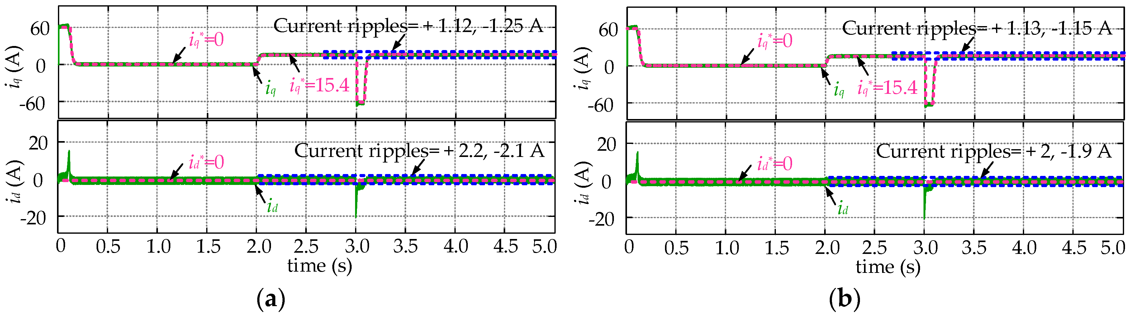
5.1. Simulation Results

The simulation setup is as follows: Between 0 and 3 s, the reference speed is set as the rated value (high speed) under no-load conditions. The rated load (5 Nm) is suddenly imposed on the shaft at 2 s, and afterward, the machine starts to decelerate to 50 rad/s from 3 s. Figure 7a shows the simulation results of case 1), and in Figure 7b, only the resistance mismatch problem is considered. As far as the individual parameter mismatch phenomenon is concerned, the proposed FCS-MPCC strategy shows significant compensation capacity. In detail, first, the d- and q-axis reference currents are nearly equal to those when no parameter disturbances appear, and the reference currents see no fluctuations, indicating that the proposed perturbation observer–based FCS-MPCC system is highly stable. Moreover, the d, q-axis current static errors are 0.05 A and −0.065 A in Figure 7a, and they are 0.05 A and −0.01 in Figure 7b. The current ripples and static errors have been greatly suppressed in comparison with those in Figure 2b and Figure 3b, although they do not completely remove the static errors. Overall, the steady-state performance has been improved greatly. Finally, during the acceleration and deceleration process, the currents can track the reference values quickly (within 0.1 s), representing that the system has remarkable dynamics.

Figure 8 illustrates the current control performance of the proposed FCS-MPCC algorithm considering the combined parameter disturbances. In these two cases, the Luenberger observer also shows excellent capacity to make the system stable and attenuate the current static errors. When both the measured resistance and inductance are smaller than the real values (as in Figure 8a), the d, q-axis current static errors are 0.05 A and −0.025 A, respectively, which are smaller than those in Figure 3c (0.2 A and −0.55 A). Compared to the traditional FCS-MPCC method, the static errors are only 0.05 A and −0.01 A when the measured parameters are larger than the real values in Figure 8b. An interesting phenomenon that should not be ignored is that the current ripples in Figure 8a are slightly larger than those for the traditional method. We believe that this phenomenon is caused by the particular parameter combination, and the proposed method is able to suppress the current ripples in most cases. Similar to the individual parameter mismatch situations, Figure 8 illustrates that the reference q-axis current is stable and approaches the desired levels.

In order to test whether the proposed perturbation observer is able to solve the other kinds of parameter mismatch problems, the simulation results concerning the flux linkage deviations (winding resistance and inductance comply with the real values) are discussed as well. The simulation setup is consistent with that in Chapter 3. Figure 9a shows the current performance when the flux linkage used for control is 0.03 Wb lower than the real values and Figure 9b shows the results when the flux linkage is 0.03 Wb higher than the real values. Although the system is still stable, obvious static errors can be witnessed. In detail, in Figure 9a, the d, q-axis current static errors are −0.7 A and 0.55 A, and they are −0.5 A and 0.5 A in Figure 9b, respectively. Figure 10 illustrates the current performance after compensation. In addition to that the system is stable as well, it is interesting to see that the static errors are greatly reduced. Specifically, the d, q-axis current static errors are −0.075 A and 0.05 A in Figure 10a and −0.15 A and 0.05 A, respectively. According to the above-mentioned analysis, although the proposed disturbance observer is proposed to tackle the resistance and inductance mismatch problems, it is capable of dealing with the other kinds of disturbances. This happens because the intrinsic properties of this kind of compensation method, which is illustrated in Section 1.

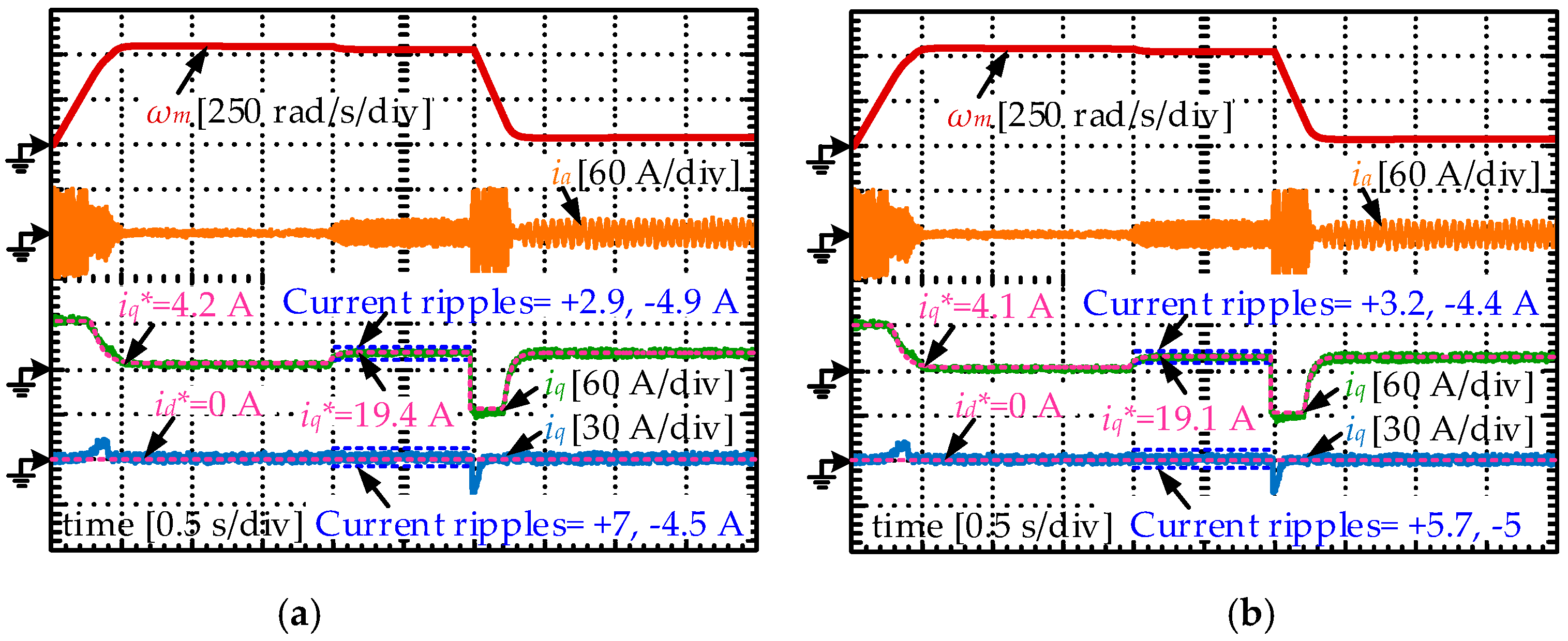
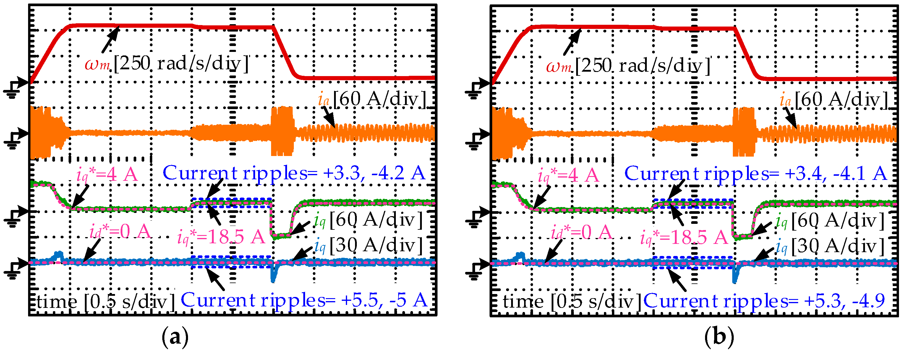
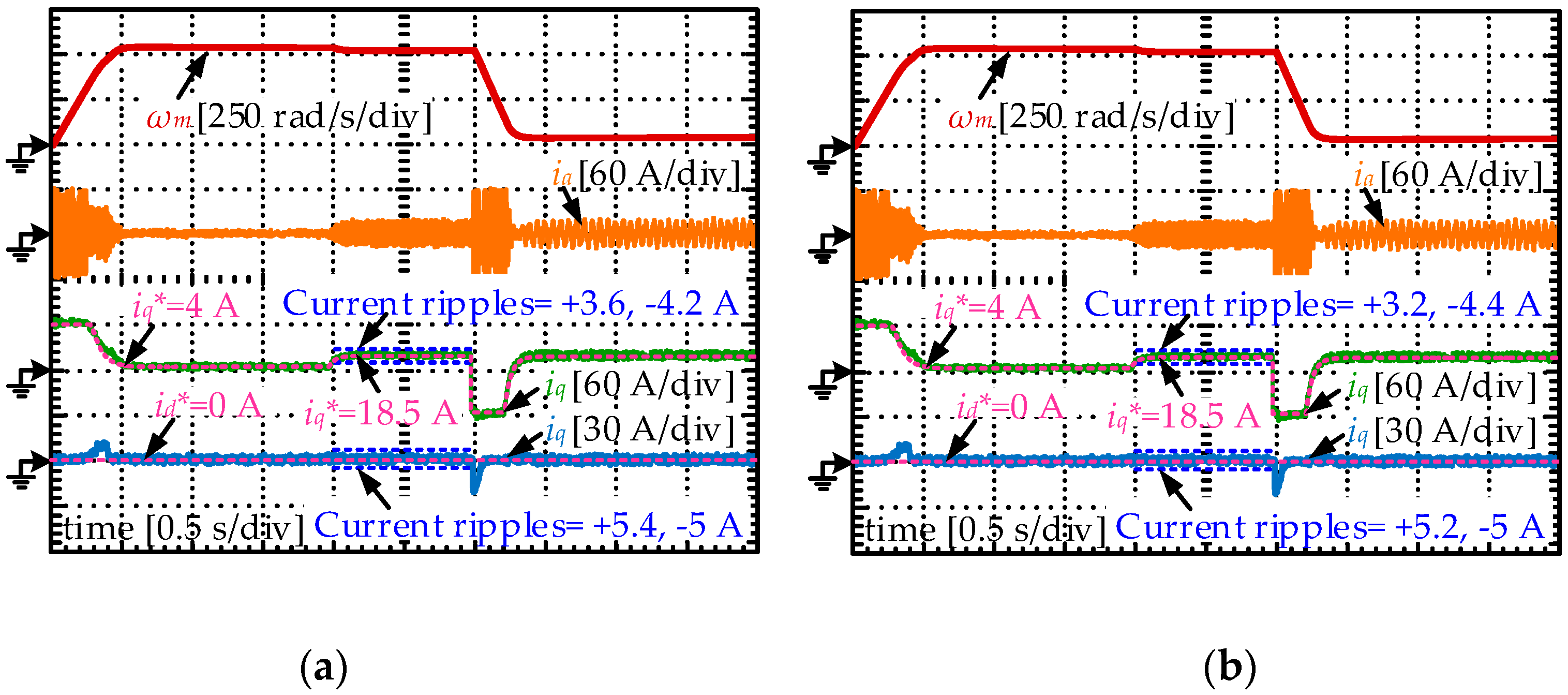
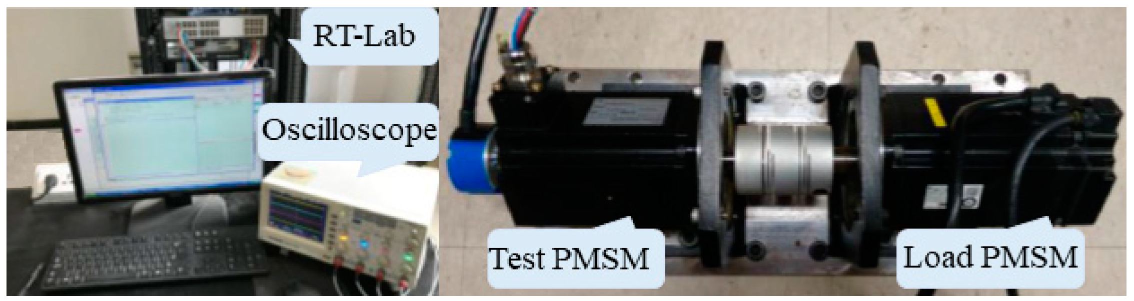
5.2. Experimental Results

The experimental setup is as follows: Between 0 and 3 s, the reference speed is set as the rated value (high speed) under no-load conditions. The rated load (5 Nm) is suddenly imposed on the shaft at 2 s, and afterwards, the machine starts to decelerate to 50 rad/s from 3 s. In order to comparatively discuss the proposed FCS-MPCC method, first, the overall control performance of the traditional PI-based double loop method (as in Figure 11a) and FCS-MPCC method (as in Figure 11b) are compared. It can be noticed that both of the strategies can keep the system stable. Then, in terms of the steady-state control performance, the current ripples of the PI-based method are slightly smaller than those of the FCS-MPCC method. This is reasonable because, for the traditional PI-based method, three voltage vectors are applied in each switching period, while there is only one voltage vector applied for the FCS-MPCC-based technique. However, in light of the easiness of an FCS-MPCC method without modulation operation, the FCS-MPCC method is still widely used in practice, and it is valuable to study this kind of control method. As far as the transient performance characteristics are concerned, speed overshoot occurs because of the intrinsic properties of the PI controllers, while no overshoot is witnessed for the FCS-MPCC-based method.

In order to explain the disturbance compensation capability of the proposed strategy. Before leaving Figure 11b, it should be noted that the d, q-axis static errors under the rated operation condition are only 0.25 A and −0.25 A, respectively. Second, the q-axis reference current generated by the speed controller are slightly higher than those in simulation (4 A for the no-load condition and 18.5 A for the loaded condition). This happens because of the viscous friction in the practical devices.

Figure 12a,b show the experimental results of case (1) and (2) under the traditional control strategy, and the control performance of the proposed strategy concerning the same cases is depicted in Figure 13a,b, respectively. First, the d, q-axis current statics errors for the traditional method in Figure 12a,b are −1 and 1.25 A, which are much larger than those in Figure 11. However, with the compensation of the disturbance observer, the current control performance in this case is similar to that without parameter disturbances. The reference q-axis currents in Figure 13a,b are both 4 A, and the current static errors stand at the same level. Finally, it should be noticed that the current ripples of the improved method are smaller than those of the traditional method in these two cases.

In terms of case (3) and (4), the control performance of the traditional method and the improved method is shown in Figure 14 and Figure 15, respectively. First, the larger current static errors can be witnessed in Figure 14. Moreover, the q-axis reference currents are 4.1 and 4.3 A for case (3) and case 4), respectively, while they are 4 A in Figure 15. Interestingly, the current ripples in Figure 14a are slightly smaller than those in Figure 15a, and as for case (4), the current ripples experience a great decrease when the proposed method is applied, which comply to the simulation results. Generally speaking, the control performance after compensation gets much more similar to that without parameter mismatch. These represent that the proposed disturbance observer can ensure high system stability, robustness, and steady-state control performance for the SPMSM FCS-MPCC controllers.

6. Conclusions

This paper proposes a Luenberger perturbation observer–based FCS-MPCC method for SPMSMs to enhance the system robustness against the winding inductance and resistance mismatch. The main contributions are as follows:

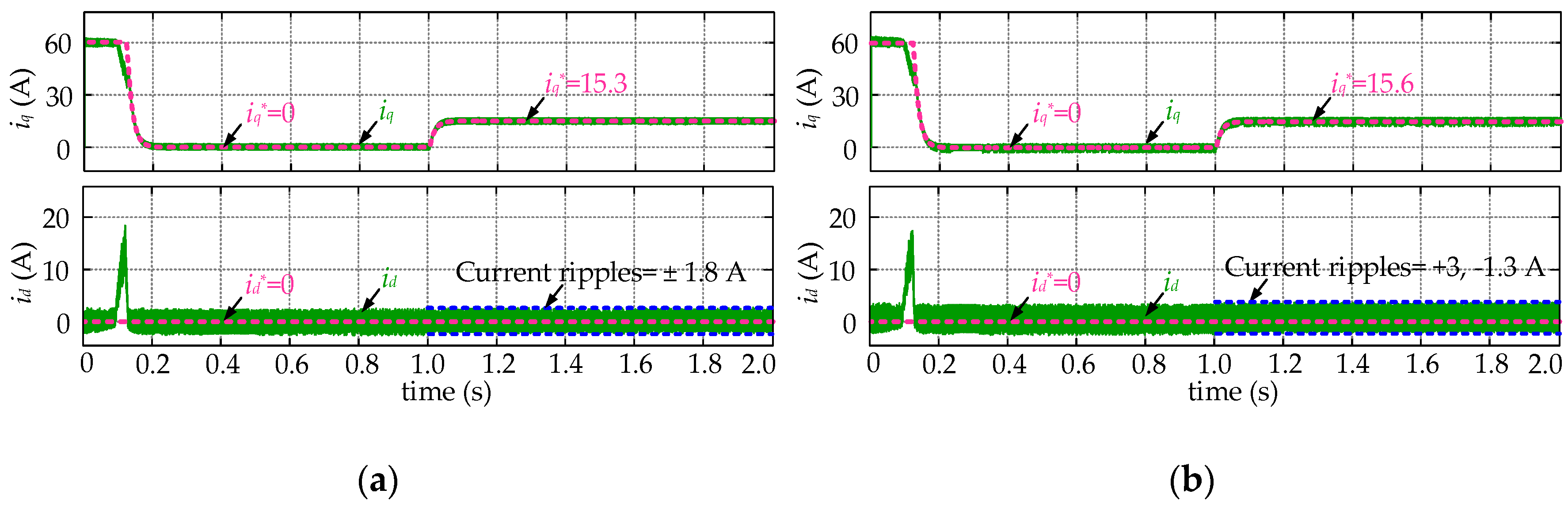
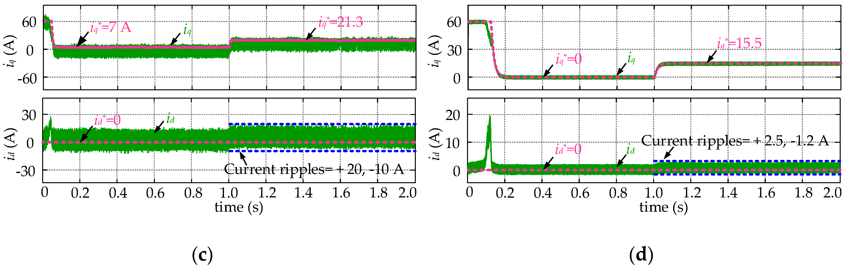
• After establishing the discrete model for the SPMSM drives and explaining the mechanism of FCS-MPCC strategies, the sensitivity of the FCS-MPCC controller to the resistance and inductance disturbances are theoretically analyzed. It is found that the parameter mismatch problem will lead to obvious control performance reduction. In detail, the current static errors grow significantly when the parameter disturbance occurs, and even worse the system stability will be influenced when the inductance deviations are sufficiently large. Therefore, the necessity to employ a disturbance observer for compensation is clarified.
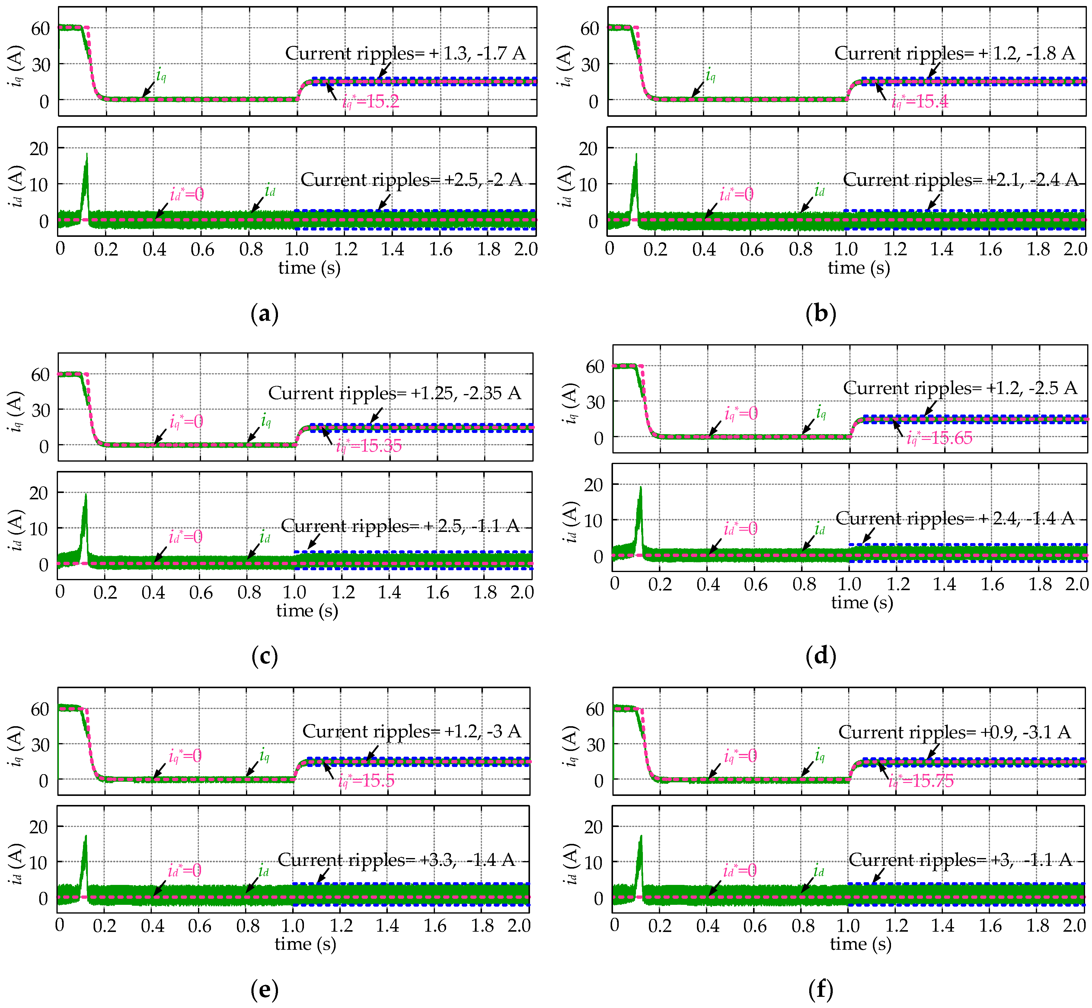
• A Lundberg observer is designed to obtain the system disturbances caused by the winding inductance and resistance mismatch problems. By using the pole assignment method, the parameters of the discrete observer are designed according to the stability condition as well as the fast response requirement. These pave the way for the relevant researches about observer-based FCS-MPCC controllers.
• The designed Luenberger observer is integrated into the prediction process of the FCS-MPCC controller to compensate the disturbances arising from parameter mismatch. Compared to the traditional FCS-MPCC algorithm, the current divergence and static errors will disappear in the parameter mismatch situations.

References

1. Liang, D.; Li, J.; Qu, R.; Kong, W. Adaptive Second-Order Sliding-Mode Observer for PMSM Sensorless Control Considering VSI Nonlinearity. IEEE Trans. Power Electron. 2018, 33, 8994–9004. [Google Scholar] [CrossRef]
2. Gong, C.; Hu, Y.; Chen, G.; Wen, H.; Wang, Z.; Ni, K. A DC-Bus Capacitor Discharge Strategy for PMSM Drive System with Large Inertia and Small System Safe Current in EVs. IEEE Trans. Ind. Inform. 2019, 15, 4709–4718. [Google Scholar] [CrossRef]
3. Wang, D.; Yuan, T.; Wang, X.; Wang, X.; Ni, Y. Performance Improvement of Servo Control System Driven by Novel PMSM-DTC Based On Fixed Sector Division Criterion. Energies 2019, 12, 2154. [Google Scholar] [CrossRef]
4. Mun, J.M.; Park, G.J.; Seo, S.; Kim, D.W.; KIM, Y.J.; Jung, S.Y. Design Characteristics of IPMSM with Wide Constant Power Speed Range for EV Traction. IEEE Trans. Magn. 2017, 53, 8105104. [Google Scholar] [CrossRef]
5. Geyer, T. Model Predictive Direct Current Control: Formulation of the Stator Current Bounds and the Concept of the Switching Horizon. IEEE Ind. Appl. Mag. 2012, 18, 47–59. [Google Scholar] [CrossRef]
6. Mynar, Z.; Vesely, L.; Vaclavek, P. PMSM Model Predictive Control with Field-Weakening Implementation. IEEE Trans. Ind. Electron. 2016, 63, 5156–5166. [Google Scholar] [CrossRef]
7. Zhang, Z.; Fang, H.; Gao, F.; Rodríguez, J.; Kennel, R. Multiple-Vector Model Predictive Power Control for Grid-Tied Wind Turbine System with Enhanced Steady-State Control Performance. IEEE Trans. Ind. Electron. 2017, 64, 6287–6298. [Google Scholar] [CrossRef]
8. Tarczewski, T.; Grzesiak, L.M. Constrained State Feedback Speed Control of PMSM Based on Model Predictive Approach. IEEE Trans. Ind. Electron. 2016, 63, 3867–3875. [Google Scholar] [CrossRef]
9. Li, H.; Lin, J.; Lu, Z. Three Vectors Model Predictive Torque Control Without Weighting Factor Based on Electromagnetic Torque Feedback Compensation. Energies 2019, 12, 1393. [Google Scholar] [CrossRef]
10. Zhang, X.; Hou, B.; Mei, Y. Deadbeat Predictive Current Control of Permanent-Magnet Synchronous Motors with Stator Current and Disturbance Observer. IEEE Trans. Power Electron. 2017, 32, 3818–3834. [Google Scholar] [CrossRef]
11. Cortes, P.; Rodriguez, J.; Silva, C.; Flores, A. Delay Compensation in Model Predictive Current Control of a Three-Phase Inverter. IEEE Trans. Ind. Electron. 2012, 59, 1323–1325. [Google Scholar] [CrossRef]
12. Scoltock, J.; Geyer, T.; Madawala, U.K. A Comparison of Model Predictive Control Schemes for MV Induction Motor Drives. IEEE Trans. Ind. Inform. 2013, 9, 909–919. [Google Scholar] [CrossRef]
13. Liu, J.; Gong, C.; Han, Z.; Yu, H. IPMSM Model Predictive Control in Flux-Weakening Operation Using an Improved Algorithm. IEEE Trans. Ind. Electron. 2018, 65, 9378–9387. [Google Scholar] [CrossRef]
14. Zhang, Y.; Yang, H. Model Predictive Torque Control of Induction Motor Drives with Optimal Duty Cycle Control. IEEE Trans. Power Electron. 2014, 29, 6593–6603. [Google Scholar] [CrossRef]
15. Zhang, Y.; Yang, H. Two-Vector-Based Model Predictive Torque Control Without Weighting Factors for Induction Motor Drives. IEEE Trans. Power Electron. 2016, 31, 1381–1390. [Google Scholar] [CrossRef]
16. Gao, J.; Gong, C.; Li, W.; Liu, J. Novel Compensation Strategy for Calculation Delay of Finite Control Set Model Predictive Current Control in PMSM. IEEE Trans. Ind. Electron. 2019, in press. [Google Scholar] [CrossRef]
17. Weihua, W.; Xi, X.; Youshuang, D. An adaptive incremental predictive current control method of PMSM. In Proceedings of the 2013 15th European Conference on Power Electronics and Applications (EPE), Lille, France, 2–6 September 2013; pp. 1–8. [Google Scholar]
18. Wang, W.; Xiao, X. Research on predictive control for PMSM based on online parameter identification. In Proceedings of the IECON 2012—38th Annual Conference on IEEE Industrial Electronics Society, Montreal, QC, Canada, 25–28 October 2012; pp. 1982–1986. [Google Scholar]
19. Wang, G.; Yang, M.; Niu, L.; Gui, X.; Xu, D. A Static Current Elimination Algorithm for PMSM Predictive Current Control. Proc. CSEE 2015, 35, 2544–2550. [Google Scholar]
20. Niu, L.; Yang, M.; Liu, K. A Predictive Current Control Scheme for Permanent Magnet Synchronous Motors. Proc. CSEE 2012, 32, 131–137. [Google Scholar]
21. Ju, Z.; Lv, X.; Wu, B.; Pu, L.; Duan, W.; Yang, P. Advanced Model Predictive Control for Three-Phase Inverter Circuit Based on Disturbance Observer. In Proceedings of the 2019 IEEE 10th International Symposium on Power Electronics for Distributed Generation Systems (PEDG), Xi’an, China, 3–6 June 2019; pp. 900–904. [Google Scholar]
22. Chen, H.; Qu, J.; Liu, B.; Xu, H. A robust predictive current control for PMSM based on extended state observer. In Proceedings of the 2015 IEEE International Conference on Cyber Technology in Automation, Control, and Intelligent Systems (CYBER), Shenyang, China, 8–12 June 2015; pp. 1698–1703. [Google Scholar]
23. Wang, B.; Chen, X.; Yu, Y.; Wang, G.; Xu, D. Robust Predictive Current Control with Online Disturbance Estimation for Induction Machine Drives. IEEE Trans. Power Electron. 2017, 32, 4663–4674. [Google Scholar] [CrossRef]
24. Wipasuramonton, P.; Zhu, Z.Q.; Howe, D. Predictive current control with current-error correction for PM brushless AC drives. IEEE Trans. Ind. Appl. 2006, 42, 1071–1079. [Google Scholar] [CrossRef]
25. Lee, K.; Park, B.; Kim, R.; Hyun, D. Robust Predictive Current Controller Based on a Disturbance Estimator in a Three-Phase Grid-Connected Inverter. IEEE Trans. Power Electron. 2012, 27, 276–283. [Google Scholar] [CrossRef]
26. Bernard, P.; Andrieu, V. Luenberger Observers for Nonautonomous Nonlinear Systems. IEEE Trans. Autom. Control 2019, 64, 270–281. [Google Scholar] [CrossRef]
27. Lu, J. Automatic Control Theory, 2nd ed.; Machinery Industry Press: Xi’an, China, 2009; pp. 238–241. [Google Scholar]
Figure 1. Block diagram of finite control set model predictive current control (FCS-MPCC) implementation.
Energies 12 03711 g001
Figure 2. Current control performance versus different measured inductance values: (a) L0 = L, ∆L = 0; (b) L0 = 2L, ∆L = −L; (c) L0 = 5L, ∆L = −4L; (d) L0 = 0.5L, ∆L = 0.5L.
Energies 12 03711 g002aEnergies 12 03711 g002b
Figure 3. Current control performance under different resistance and inductance set values: (a) L0 = L, ∆L = 0, Rs0 = 0.5Rs, ∆Rs = 0.5Rs; (b) L0 = L, ∆L = 0, Rs0=5Rs, ∆Rs = −4Rs; (c) L0 = 0.5L, ∆L = 0.5L, Rs0 = 0.5Rs, ∆Rs = 0.5Rs; (d) L0 = 0.5L, ∆L = 0.5L, Rs0 = 5Rs, ∆Rs = −4Rs; (e) L0 = 2L, ∆L = −L, Rs0 = 0.5Rs, ∆Rs = 0.5Rs; (f) L0 = 2L, ∆L = −L, Rs0 = 5Rs, ∆Rs = −4Rs.
Energies 12 03711 g003
Figure 4. Block diagram of the proposed disturbance observer.
Energies 12 03711 g004
Figure 5. Block diagram of the robust observer-based FCS-MPCC strategy.
Energies 12 03711 g005
Figure 6. Test bench.
Energies 12 03711 g006
Figure 7. Current control performance of the proposed FCS-MPCC method under different resistance and inductance disturbances: (a) L0 = 2L, ∆L = −L, Rs0 = Rs, ∆Rs = 0; (b) L0 = L, ∆L = 0, Rs0 = 5Rs, ∆Rs = −4Rs.
Energies 12 03711 g007
Figure 8. Current control performance of the proposed FCS-MPCC method under different resistance and inductance disturbances: (a) L0 = 0.5L, ∆L = 0.5L, Rs0 = 0.5Rs, ∆Rs = 0.5 Rs; (b) L0 = 2L, ∆L = −L, Rs0 = 5Rs, ∆Rs = −4Rs.
Energies 12 03711 g008
Figure 9. Current control performance of FCS-MPCC without disturbance compensation under different flux linkage disturbances: (a) Flux linkage used for control decreases 0.03 Wb (0.045 Wb); (b) Flux linkage used for control increases 0.03 Wb (0.105 Wb).
Energies 12 03711 g009
Figure 10. Current control performance of proposed FCS-MPCC with disturbance compensation under different flux linkage disturbances: (a) Flux linkage for control decreases 0.03 Wb (0.045 Wb); (b) Flux linkage for control increases 0.03 Wb (0.105 Wb).
Energies 12 03711 g010
Figure 11. Experimental results under no parameter disturbances: (a) Traditional proportional integrate (PI)-based method. (b) FCS-MPCC method.
Energies 12 03711 g011aEnergies 12 03711 g011b
Figure 12. Experimental results of the traditional FCS-MPCC method under different resistance and inductance disturbances: (a) L0 = 2L, ∆L = −L, Rs0=Rs, ∆Rs = 0; (b) L0 = L, ∆L = 0, Rs0 = 5Rs, ∆Rs = −4Rs.
Energies 12 03711 g012
Figure 13. Experimental results of the proposed FCS-MPCC method under different resistance and inductance disturbances: (a) L0 = 2L, ∆L = −L, Rs0 = Rs, ∆Rs = 0; (b) L0 = L, ∆L = 0, Rs0 = 5Rs, ∆Rs = −4Rs.
Energies 12 03711 g013
Figure 14. Experimental results of the traditional FCS-MPCC method under different resistance and inductance disturbances: (a) L0 = 0.5L, ∆L = 0.5L, Rs0 = 0.5Rs, ∆Rs = 0.5 Rs; (b) L0 = 2L, ∆L = −L, Rs0 = 5Rs, ∆Rs = −4Rs.
Energies 12 03711 g014
Figure 15. Experimental results of the proposed FCS-MPCC method under different resistance and inductance disturbances: (a) L0 = 0.5L, ∆L = 0.5L, Rs0 = 0.5Rs, ∆Rs = 0.5 Rs; (b) L0 = 2L, ∆L = −L, Rs0 = 5Rs, ∆Rs = −4Rs.
Energies 12 03711 g015