Article

Analysis Application of Controllable Load Appliances Management in a Smart Home

by
Gerardo J. Osório
1,
Miadreza Shafie-khah
2,*,
Gonçalo C. R. Carvalho
3 and
João P. S. Catalão
3,4
1
C-MAST, University of Beira Interior, Calcada Fonte Lameiro, 6201-001 Covilha, Portugal
2
School of Technology and Innovations, University of Vaasa, 65200 Vaasa, Finland
3
Faculty of Engineering of University of Porto, R. Dr. Roberto Frias, 4200-465 Porto, Portugal
4
INESC-TEC, R. Dr. Roberto Frias, 4200-465 Porto, Portugal
*
Author to whom correspondence should be addressed.
Energies 2019, 12(19), 3710; https://doi.org/10.3390/en12193710
Submission received: 5 August 2019 / Revised: 19 September 2019 / Accepted: 26 September 2019 / Published: 27 September 2019
(This article belongs to the Special Issue Intelligent Energy Systems)

Abstract

:
The residential sector is one of the sectors with the highest rates of electricity consumption worldwide. For years, many studies have been presented in order to minimize energy consumption at the residential level. The idea of such studies is that the residential customer (RC) is the interested party of their own consumption. Moreover, the algorithms that have been developed to predict and manage the energy consumption, also analyze the behavior of the loads, with the objective of minimizing the energy costs, with good safety, robustness, and comfort levels. In the context of the smart house (SH), one of the objectives of smart grids (SGs) is to enable the RC, with home energy management systems (HEM), to actively participate, allowing for higher reliability at different levels. In this work, a new model that simulates the behavior of an SH, considering heating, ventilation and air conditioning (HVAC) and sanitarian water heater (SWH) devices, is presented. For this purpose, the proposed model considers realistic physical parameters of the SH, together with customer comfort, in order to mitigate the RC disinterest. The proposed model considers the electric vehicle (EV), a battery-based energy storage system (ESS), a micro production unit, and different types of tariffs that the RC might choose, aiming to maximize the benefits, and temporarily shifting the proposed loads.

1. Introduction

1.1. Framework and the State-of-the-Art

Nowadays, there is a need to optimize the energy consumption of houses in order to minimize the energy costs and reduce the greenhouse gas emissions. For that purpose, the European Union members are increasing renewable energy production, starting with more variable power generation [1]. It is at this point that a new concept emerges—the concept of the smart house (SH).
The SH is a technology where everything can be controlled and monitored in different areas, such as home appliances, energy-consuming devices such as heating, ventilation and air conditioning (HVAC), dishwashers, washers and dryers, all through the use of networks [2]. The consumers have access to in-house device controllers, which results in a better quality of life and better cost saving. In the last decade, a competitive energy market has been established. During the day, there is a variation in the energy prices which facilitates the idea of buying electricity when it is cheaper. Based on that, SHs are being integrated into a smart grid (SG) eco-system, in terms of the households’ energy consumption and management [3].
Therefore, it is necessary to create a scheme where it is possible to change the power consumption of a residential customer (RC), to better match the demand with the supply.
An SH provides an RC with sophisticated monitoring and control, over the house equipment, through advanced automation systems. An SH should have an integrated prediction mechanism, and an algorithm for decision making, human–machine interface, with wireless networking, amongst others [4,5]. Any device in an RC house that uses electricity can be put on the RC home’s network under the RC’s command, i.e., when the RC gives the order, the SH reacts.
Most applications are related to lighting, home security, home theatre and entertainment, and thermostat regulation. SHs also include security, medical treatment, data processing, entertainment, and businesses at home [6]. SHs are able to record the consumption of different electrical appliances by use of a smart meter. However, RCs are reluctant to have smart meters mainly because of the costs involved [7]. Along with the electrical installations, SHs include network setups such as wireless and ZigBee® (Zigbee Alliance, Davis, California, USA). However, there are several meanings of the term SH. SH can be divided into three technological groups, all of them with the main goals of improving the automation process and reducing the final consumption [8].
The first group is considered as the group with devices that are controlled remotely, with the equipment connected to each other. The second group consists of the programmable houses where the purpose is to adapt, according to different types of input sensors, and to recognize certain situations. Finally, the third group of the SHs aim to recognize patterns and react to the inputs. All of these developments, and automation in this field, will help RCs, and other electrical players, to reduce their Internet bill and optimize the electricity bidding and prices by conducting load management through the SH.
With the help of a smart phone or a laptop, loads can be managed remotely to help the RC to control and manage the energy and equipment and, as a result, reduce the energy bill. Every load has a different type of operation, so it becomes necessary to separate the different type of loads into the critical loads and controllable loads [9].
Critical loads are lighting, refrigeration and freezing. The controllable loads can be divided into thermostatically controlled and non-thermostatically controlled. In the first group are the HVACs and sanitarian water heater (SWH). For these, two different types of loads, and a set temperature needs to be chosen, whether by the consumer or the program [10]. The non-thermostatically controlled loads are the dishwashers, washers, dryers, plug-in hybrid EV, and other equipment that does not need to have a set temperature.
The market for EVs is growing and they are becoming more and more common [11]. One of the EV advantages, in an SH, is the flexibility given by considering the charging/discharging schedule. This means that the charging/discharging of the EV can be scheduled at specific times in order to avoid the energy peak [12] thereby benefiting the consumer. The EV linked to an SH has the ability to stop the charging and continue it when it is convenient. Another ability of the EV is the capability of not only having the operation of the grid to the vehicle (G2V), but also the vehicle to the grid (V2G) [13]. This means that when the grid needs it, the EV can also work as a battery that sells energy to the grid, i.e., as a bidirectional power flow, helping in the control of the power peak.
Moreover, there are different ways of achieving the goal of lowering the energy price and peak load, by adopting several types of load management. One of them is load shifting, where loads that are independent of time, and cause minimal inconvenience, are shifted from peak time to another period of time where the grid load is lower, ensuring that certain equipment will work when the price is lower. Another type of load management is through conservation, where the overall goal is to reduce the energy consumption. This type of management will maintain the shape of the daily consumption, reducing the power every hour, or at least for most of them. The last one is peak clipping, where the system will limit the power consumption to an upper limit, turning off the equipment when the power reaches that limit [14].
The load shifting can be divided into three, without shifting, power shifting, and time shifting. Power shifting is related to the change of the loading pattern, e.g., charging of the EV, which will be divided into different periods throughout the day. The time shifting will change the start and end time to allow a better allocation of the loads [15]. However, time shifting is limited and it can be applied to the dishwashers, dryers, and washing machines.

1.2. Benefits and Risks of a Smart House and Demand Response Concept

SHs guarantee benefits to both the electricity suppliers and the RCs [16]. The authors of [17] conducted a study that showed the multiple benefits of an SH, compared to a non-SH, with real experimental values. It was proven that the RC, with an SH, had accurate billing information, helping to reduce the energy costs and helping the consumer to regulate his/her behavior while using a variety of technology. The communication between the energy supplier and the RC is essential due to the suppliers’ knowledge of the energy market mechanisms and the different energy rates.
The authors of [18] described the numerous benefits of an SH which can improve the RCs’ lifestyle. An SH can save energy, make things easier, save time and money, provide comfort, and improve the quality of life and leisure. Hence, SHs also can provide healthcare for individuals, especially for older people, making it possible to measure the vital signs of people in their own home [19]. However, there are some associated risks, such as the increased dependence on the technology, the increased dependence on the electricity networks, and the possibility of privacy invasion, amongst others [18].
One of the biggest problems is achieving the necessary security, which has been the major problem for SH implementation. Integrating security-enhancing methods is difficult because the design is not linear, and it requires substantial investigation and investment. For instance, in [20], a risk analysis in an SH automation system was performed, and the results showed that with the implementation of standard measures, the risks can be minimized to acceptable levels. Security needs to be achieved in different categories:
  • Confidentiality—the guarantee that the data will be disclosed only to authorized entities or systems. This means that only authorized people are allowed to access certain information;
  • Integrity—the guarantee that the accuracy and consistency of the data will be maintained. No unauthorized modifications, destruction, or losses of data will go undetected;
  • Availability—the assurance that any network resource (data/bandwidth/equipment) will always be available for any authorized entity. Such resources have to also be protected against any incident that threatens their availability;
  • Authenticity and authorization—the validation that communicating parties are, who they claim they are, and that messages supposedly sent by them are indeed sent by them;
  • Non repudiation—undeniable proof to verify the truthfulness of any claim of an entity [21]. In order to minimize the energy costs, the SHs have programs that help users to reduce their expenses. These programs are called demand response (DR) programs.
DR, as explained by the authors of [22], can be divided in two groups: DR-based on prices (PBDR), and DR-based on incentives, (IBDR) programs. The IBDR programs are classified into three groups: voluntary effort, the market clearing programs, and the price based programs. A DR program introduces load flexibility, where different entities will benefit, starting with RCs and the electricity supplier [23]. The main goal of these DR programs is to regulate the operational and economical parameters of the power system [24]. PBDR programs are capable of offering a scheme based on the price variation. As an example, the real-time pricing (RTP) scheme is able to “transport” the wholesale market principles into the retail market.
RCs can benefit from an electricity bill reduction if the RCs adjust their demand according to the prices. RCs are informed about the tariffs an hour ahead of time, in order to adjust their loads [25]. Another price-based DR, the time-of-use (TOU) pricing, is an electricity model that changes with the time of day. This tariff is low in off-peak, moderate in mid-peak and high in peak-periods. TOU also includes the seasonal variation of the energy consumption [26]. TOU pricing is more practical than real-time pricing (RTP) for most consumers, and reduces the efficiency of single pricing [27]. Moreover, the objective of the critical-peak pricing (CPP) program is to drastically reduce the load during the few intervals where the price is very high [28].

1.3. Related Works Considering Management of Controllable Appliances in a Smart Home

The efforts and widespread information in this field of knowledge is notable, however, there are several factors, as stated in previous section, that influence the general acceptance of SH, and in this sense, it is not yet a mature field [29]. In this trend of HEM approaches, considering controllable loads and other RC inputs, such as tariff, RC comfort, among others, several examples can be obtained. For instance, in [30], the optimal operation of a neighborhood of SHs in terms of minimizing the total energy cost was analyzed, considering several levels of facilities in an SH, some technological communication options, different tariffs and several safety constraints. The proposed approach demonstrated that RCs would be incentivized to shift their consumption in order to achieve lower electricity bills, and called for a smoother introduction of SH in order to reduce their impacts.
In [31], a real-time appliance-based HEM approach was proposed considering an appliance control algorithm modeled through Petri nets, in a priority order, to reduce the electricity bill and improve the energy efficiency, keeping the user comfortable. The results showed significant reduction in the consumption, final bill cost and peak load reduction.
In [32], a two-level HEM framework was proposed. In the first level, RCs run an optimization model to minimize the payment cost, forwarding the desired operational scheduling results to the system operator. In the second level, a multi objective optimization model is described in order to improve the reliability of the distribution system considering the load demand deviation, given the least desired payment cost of each RC. It was demonstrated that the proposed HEM program reduced the distribution peak load, as well as the system losses, compared to the same case without the HEM strategy.
In [33], the concepts of the contemporary house with SH technology was presented and a literature review was carried out on SHs research related to energy management within the RCs and network system. From this research, it was determined that higher considerations of the SH features are needed, in terms of real applications and new socio-technical outlines. The authors of [34] proposed an information gap decision theory model for robust HEM, considering the summer season in the presence of market price fluctuation scenario. To this end, the optimization problem of low-energy SH was modeled considering the risks and formulated as a mixed-integer non-linear programming.
In [34], a novel incentive-based HEM model was proposed to manage the community demand reduction requests proficiently, rewarding RCs with the needed comfort and multi-level financial incentives. To this end, a new comfort sign was proposed which takes into consideration thermal and major controllable appliances. The proposed model was structured by a genetic algorithm structure in order to minimize the rewarded costs and maximize the RCs’ comfort level. Moreover, a mixed integer model was used for comparison analysis, and it was concluded that the proposed approach outperformed in terms of reward incentives, comfort levels, and the number of active appliances.
In [35], a social welfare maximization model was proposed based on Markov decision process, considering the features matrix that describes the elasticity appliances available in the SH, as well as several state transfer functions to highlight the semi-elastic appliances. Moreover, in order to guarantee the RCs’ privacy, the model was divided into two sub-problems, i.e., RCs and suppliers. From the RCs’ perspective, a modified decentralized RTP algorithm was developed to solve the optimization problem. To consider the supplier perspectives, the dual sub-gradient technique was implemented to compute the convex optimization problem in the paper.
Moreover, in [36] a scheduling model of RC appliances considering appliances’ features as well as the RC comfort was considered by a bottom-up engineering model, in order to obtain an enhanced understanding of residential electricity demand patterns. To cover the nonlinear complex combinatorial problem, an improved cooperative heuristic approach was proposed to achieve a near optimal solution with enhanced outputs.
In [37], an incentive-based demand management model for schedulable appliances was proposed, with the goal of creating scalability to the system. To this end, a compensation scheme was adopted for load appliances shifting, based on the awkwardness level. Moreover, different demand reduction events within a month were analyzed with the proposed scheme, considering the outputs through TOU tariff, and a base case model. The reported results demonstrated that the proposed model might save 11.3% in comparison to the base case, and 6.2%, on average, considering TOU tariff-based optimization.
Recently, more contributions considering controllable load appliances management in an SH have been proposed. An example of this is found in [38], where the strategy of smart energy management system was proposed to deal with the scenario of a complete power outage in an area with partial load shedding, as well as taking into consideration RCs’ preferences. To this end, DR strategies were also applied, through the maximum demand bound levels, changing the priorities assigned to an appliance. Cost optimization models based on TOU, RC comfort level and sensoring data were included in the proposed model.
In [39], a HEM model was presented, considering linear programming, in order to adjust the power of thermostatically controlled loads (specifically the HVAC system) together with photovoltaic-battery ESS. The HVAC system was initially calculated considering variable home temperatures, while the HVAC consumption was estimated using degree-days. Moreover, the output from photovoltaic-battery ESS was computed considering technical parameters, i.e., solar irradiances and ambient temperatures. The proposed HEM demonstrated a significant energy reduction by 30%, maintaining the RC’s comfort, as well as guaranteeing the ESS lifetime and operational constraints.
The authors of [40] analyzed the definition concerning the concepts of smart city and smart commodities and facilities. The main goal here was understanding, and capturing the essence of meaning of smart concepts, so as to address or easily show the impacts on future smart stakeholder participants. The research analyses demonstrated that further and deeper collaboration between the information and communication technologies and social–economic research fields is crucial, and should be started and combined in a viable manner, in order to satisfy the participants’ needs in a smart concept reality.
In the same vein, the authors of [41] presented a text mining model to create an accurate understanding about smart services definitions, through a combination of metrics and machine learning concepts. The aim was to analyze the text data related to smart service systems from the widespread scientific literature in recent years, with the main goal of creating a base concept across multiple disciplinary overviews for the future of smart systems research proposals.

1.4. Goals, Contributions and Structure

The present work aims to study the functioning of an SH, with limited resources, and equipped with a wind micro turbine, EV energy-exchange possibility, and a battery-based ESS. The possibility of selling back to the grid, within the line limit parameters is also including, taking into consideration:
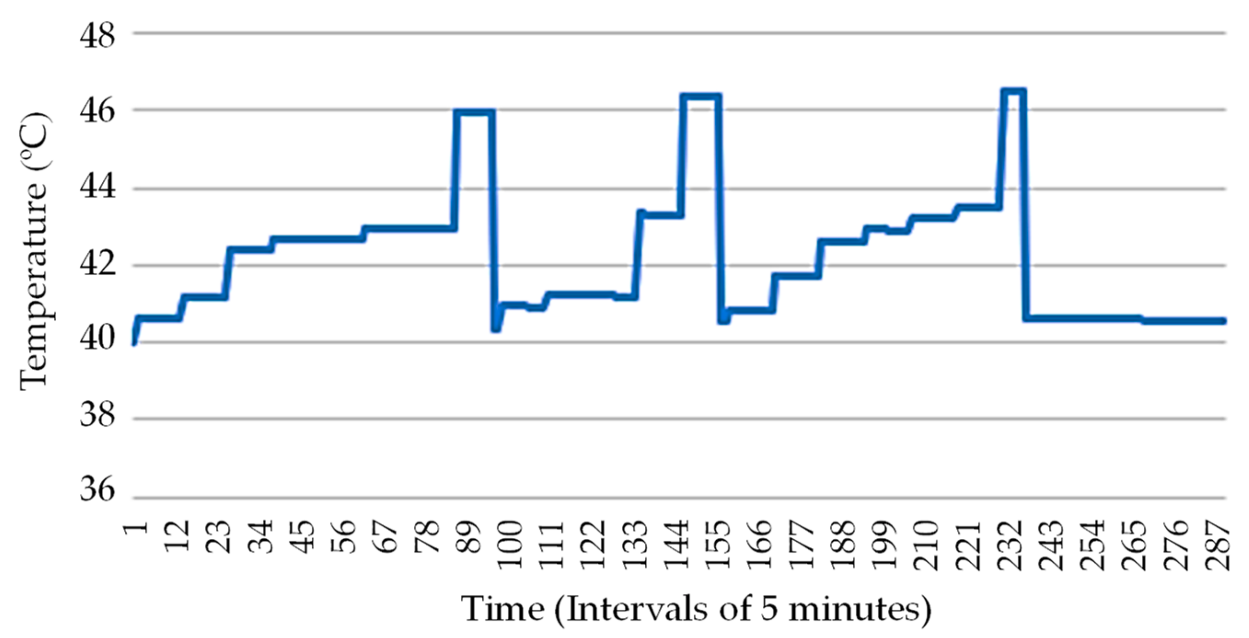
  • The evaluation of the load distribution of the SWH for each tariff under analysis;
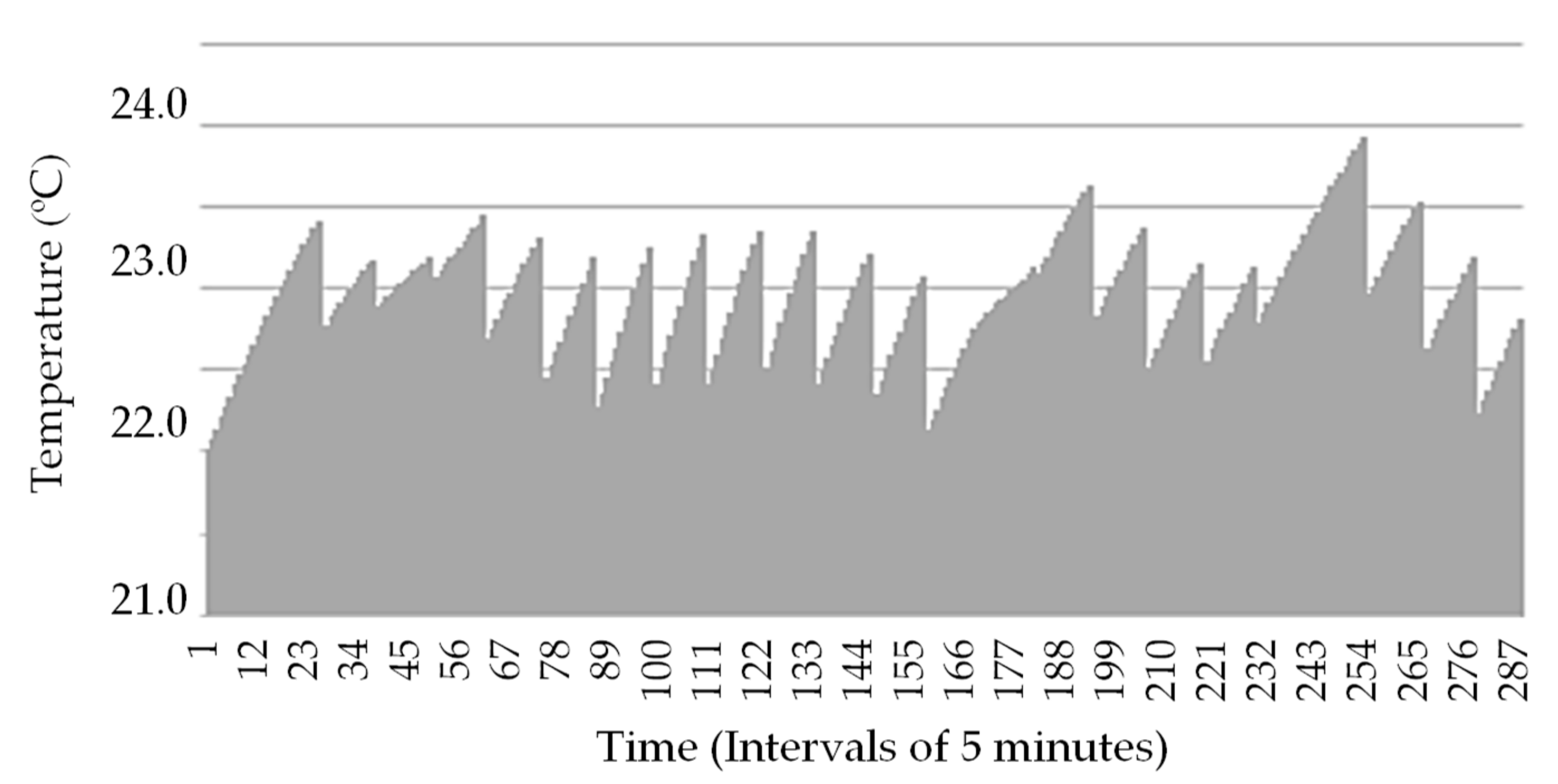
  • The evaluation of the load distribution of the HVAC system, in cooling mode, for each tariff;
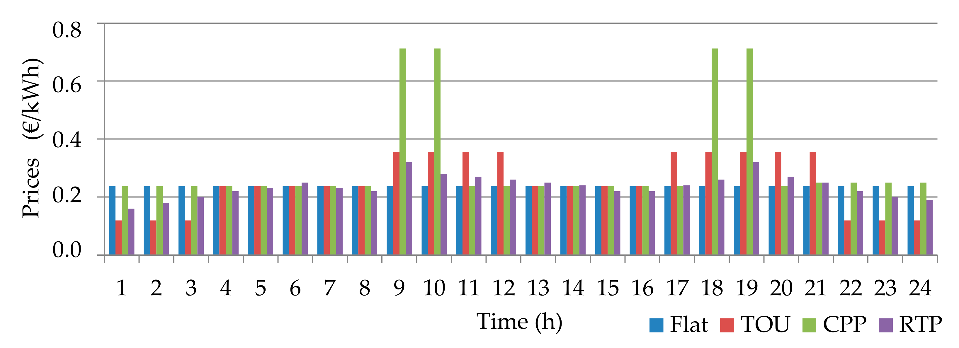
  • The evaluation of the cost/profit associated for each tariff (flat price, TOU, RTP, and CPP schemes).
In this sense, and following the latest trend in this field of knowledge, this work proposes a HEM model analysis to improve the efficiency and reliability, with increased integration of SH concepts and controllable loads as SWH and HVAC systems. The problem is addressed from the RC’s point-of-view, unlike most existing approaches in the scientific literature, which take the system operator’s point-of-view.
A two-stage stochastic management model analysis was developed. The first stage is the day-ahead market, where the price of the trade is set for the next-day, and the second stage, or the RTP, is where the energy can be traded in real-time, which gives different prices to the day-ahead model. On this proposed model, some stochastic parameters that correspond to wind generation have been implemented, due to the natural uncertainty of the wind behavior.
So, the objective and main goal of this work is also related to the implementation of an algorithm that allows for a physical-based model analysis of the SWH and HVAC systems, and their usage, in order to minimize the power consumption/energy cost, while still adequately taking into consideration the RCs’ comfort. For the interpretation and analysis of the results obtained in the modeling of the proposed problem, several case studies (with different tariffs) are considered for an extensive analysis. The remaining manuscript is organized as follows: Section 2 presents the methodology and mathematical formulation considered in the proposed model; Section 3 presents the case studies, the results, comparison and discussion analysis; Section 4 lists the main conclusions drawn in this work and Section 5 shows the future directions that might be conducted from the current work.

2. Mathematical Formulation

In this section, the mathematical formulation that defines the cost or revenue for the RC will be presented. Moreover, the mathematical formulation necessary to correlate the relation between the SH consumption and the exchanges with the network, will also be presented. The different constraints of both the SH, and the network, are also formulated.
As stated before, the model used in this work runs under a stochastic programming, and it is divided into two different stages. The first stage is the day-ahead market, where the price of the trade is set for the next-day, and the second stage, or the RTP, is where the energy can be traded in real-time, with different prices to the day-ahead model. Moreover, some stochastic parameters from wind power generation have been considered, due to the natural uncertainty and volatility of the wind behavior. Then, the physical-based model of the house has been obtained, in order to understand in which way the energy usage increases for the controllable loads under study, i.e., the SWH and HVAC systems, and based on their features, the goals are to minimize the power consumption/energy cost, as well as satisfy the RCs’ comfort.

2.1. Objetive Function and Market Pricing Modelling

The objective function is the minimization of the total expected cost (EC), or increase of the expected profit (EP), by selling/purchasing energy to/from the day-ahead and the real-time market. The objective function will consider the first and second stages, the day-ahead and the real-time stages, respectively. In Equation (1) the EP or EC consists of two parts. The first part is the EP due to the energy trade with the day-ahead local market (LM).
The second part of the equation represents the profit of the exchanged energy in the real-time market. This is related to the energy revenue, the energy cost, the wind spillage cost, and the load shedding costs of the SWH and HVAC systems. Note that in this formulation, the cost of the battery-based ESS and the EV are equal to zero, because it is a HEM problem analysis only [42].
For the first stage, the day-ahead market is considered where the variables are only related to the day-ahead market, and where the different wind power scenarios are not considered. For the second stage, 10 different wind power scenarios are considered, with each wind power scenario having the same equiprobability, i.e., π w = 10 %. Moreover, the wind micro-turbine, ESS, and EV, are the energy resources in the house.
The HVAC system is considered as a thermostat programmable controllable load, the SWH tank is considered as a thermostat controllable and shiftable load, and the must-run services are considered as non-dispatchable loads, without considering the uncertainty of this type of load [43].
E P = t λ t d a P t n e t ,   d a + t π w t λ t s o l d ,   r t P t w s o l d ,   r t λ t p u r , r t P t w p u r ,   r t V S S t w
Equation (2) represents the power balance equation due to the power output of the wind micro-turbine, the discharged power of the ESS, the discharged power of the EV, the charge power of the ESS, the charged power of the EV, the traded energy with the LM, the predicted values of the SWH, and HVAC systems, and the must-run services. Equation (3) represents the limit of power in the lines, in both directions. On the day-ahead market, in contrast to the RTP scheme, only the forecasted values are considered. Moreover, Equation (4) represents the energy traded with the day-ahead market, based on the wind power point forecast.
P t w i n d ,   d a + γ b P t b ,   d i s ,   d a + γ e v P t e v ,   d i s ,   d a = L t h v a c ,   p r e d ,   d a + L t s w h ,   p r e d , d a + L t m r s ,   p r e d ,   d a +   γ b P t w b ,   c h ,   d a + γ e v P t e v ,   c h ,   d a + P t n e t ,   d a
f m a x P t n e t ,   d a f m a x
P t n e t ,   d a = P t w i n d ,   p r e d
Equation (5) represents the power equation of the SH, in real-time. The values of energy consumption by the HVAC system and the SWH tank are calculated based on the algorithms that will presented in the next sub-section. The energy balance is performed every 5 min in order to incorporate the values obtained for the HVAC system and the SWH tank models. These models need to calculate values every 5–10 min in order to accurately model these loads.
Equation (6) expresses the load balances on the SH exchange lines with the SG. The sum of the values of the energy exchanges with the network must obey the constraints of the maximum limits of the line. Equation (7) represents the maximum value of the sold energy in the real-time market and the energy consumed in the real-time market following the respective constraints.
P t w w i n d , r t + P t w b ,   d i s ,   r t + P t w e v ,   d i s ,   r t + P t w p u r ,   r t = L t w s h d , r t + L t w s w d , r t + L t w m r s ,   r t + P t w b ,   c h ,   r t + P t w e v ,   c h ,   r t + P t w n e t ,   d a + P t w s o l d ,   r t
f m a x P t w n e t ,   d a + P t w s o l d ,   r t + P t w p u r ,   r t f m a x ,   t T ,   w W
P t w s o l d ,   r t + P t w p u r ,   r t f m a x ,   t T ,   w W

2.2. Sanitary Water Heating Load Model

The following equations represent the SWH model [44].
T t + 1 h ,   w = T t a + Q × R × u t S W H T t a T t h ,   w e Δ T R . C ,   t < T m a x ,     m t = 0
T t + 1 h ,   w = T t h ,   w 0.26417 M m t + T t c , w × m t 0.26417 M ,   t < T m a x ,     m t > 0
T h ,   w ,   m i n T t h , w T h ,   w ,   m a x ,   t T
T t m i n w s < T t h ,   w < T h ,   w ,   m a x ,   m t > 0 ,   t T
P t S W H = Q × u t S W H ,   t T
Equation (8) is represents when the hot water from the SWH tank is not being used, meaning that, for instance, no one is using the shower at that moment and that the temperature is decreasing slowly overtime. However, if the temperature is not appropriate, the system will run automatically to elevate the temperature within the desired range.
Analogously, Equation (9) represents when the hot water from SWH is being used, assuming three daily periods, which maybe related to three baths at different times. During these 10-min time periods, the SWH tank is programmed not to warm up for safety reasons.
Equation (10) models the limits of the temperature for each time slot. The temperature should be between 40   ° C and 6 0   ° C . Equation (11) shows the temperature limits during the bath of the RC, and should be up to 4 0   ° C , for comfort reasons. Equation (12) is related to the power consumed while the SWH tank is working. Parameter P t S W H , (the demand for electricity of the SWH tank), shows the energy consumed for each time slot.

2.3. Heating, Ventilation and Air Conditioning Load Model

The following equations represent the HVAC model [45]. For the HVAC system first, the temperature in the room is calculated as follows:
T t r = 1 Δ t 1000 M a c a R e q T t 1 r + Δ t 1000 M a c a R e q T t 1 a u t 1 H V A C C O P × P H V A C Δ T 1000 M a c a R e q ,       t > 1
S P t S t d T t r S P t + S P t u ,     t > 1 : S P t N a N
P t H V A C = P H V A C × u t H V A C ,     t   T
Equation (13) is the calculation of the temperature in the room in each time slot. The binary variable (ON/OFF) will change to keep the temperature between acceptable values. The dead-band is considered 1   ° C and means that the HVAC output temperature may vary by 1   ° C above or 1   ° C below the expected value.
Equation (14) formulates the restrictions of the temperature deviations. Equation (15) expresses the power spent on the HVAC system, which will not be 0, only if the HVAC is working on that period.

3. Case Study and Results Analysis

3.1. Details, Data, and System Considered

The model proposed was implemented using the General Algebraic Modeling System (GAMS) [46]. The implementation was made on a standard PC (8 GB RAM, Intel Core i5 2.7 GHz, Windows 7 OS, Microsoft, Redmond, WA, USA). Compilation time required was less than 10 s. Pre- and post-processing of the results was performed using MS Excel. Hence, the proposed model connects the LM with the proposed domestic energy management (DEM) system. The SH is capable of buying and selling energy with the LM, and it is equipped with battery-based ESS and EV. The DEM system also considers the behavior of a wind micro-turbine with the maximum capacity of 2 kWh.
The ESS can store between 0.48 and 2.4 kWh, with the maximum charge and discharge rate of 400 W, with a charge/discharge efficiency of 90%. The EV is capable of storing 1.77 and 5.9 kWh, with a charging/discharging rate of 3 kW, while the charging/discharging efficiency was rated at 90%. The EV is scheduled to leave home at 07:00 and returns at 17:00. Moreover, the EV is programmed for the worst case scenario, which means that when it returns home it is “out-of-charge” and that at 07:00 a.m., the EV needs to be fully charged. Moreover, the loss of energy between electric appliances is considered to be null.
Due to the unpredictability of wind power, a stochastic parameter of the wind has been created. The wind parameterization has been done for different scenarios with an associated probability, shown in Figure 1. Figure 2 describes the stochastic results from the predicted values of the HVAC system in the day-ahead market, and Figure 3 expresses the stochastic results from the predicted values of the SWH tank, from the day-ahead market.
To this end, T c , w t is considered the same as the room temperature calculated by Equation (13). The hot water flow rate is simplified as an average value of 2.5 gallons (in this work it was converted to liters) per minute, which is the normal average consumption in a typical house. For the sake of simplicity, the exterior temperature was considered to be 20 °C.
For the parameters R , C , M (capacity in litres), the values above were considered, which are the typical values for a SWH tank. The value of Q is a typical value for the SWH power, which is 2 kWh. The time interval was in minutes so, Δ t is 5/60. The showers are scheduled to be used at 07:50 a.m., 13:30 p.m., and 20:30 p.m., with a 10-min duration. During that time, the minimum hot water temperature is 20 °C, and the maximum is always 60 °C, for safety reasons.
However, the minimum temperature in the SWH tank, when the consumers are using hot water, is 40 °C for safety and comfort reasons. So, when showers are being taken, the temperature is always between 40 °C and lower than 60 °C. The binary variable u t S W H from Equation (8) was 1 or 0, in order to maintain the temperature in the SWH tank within viable values.
For this calculation, an interval of temperatures is chosen and the SWH tank turns ON/OFF to maintain the values of the intervals, making the temperatures always around the temperature set-point. The exterior temperature is expressed in Figure 4. For this analysis, Δ t was considered as the dead-band, with ±1 °C and constant.
The value of S P t is the thermostat set-point and S t d is the value of the maximum deviation. Normally, the density of the air and its thermal capacity depends on its thermodynamic properties (temperature, pressure, amongst others). However, for the sake of simplicity, in this model, such parameters were considered constant and we utilized standard values: ρ a r       =   1.225 kg/m3, and c a   =   1.010 kJ/kg°C. The equivalent thermal resistance was 3.1965 ×   10 6 °C h/J.
The mass of air was 1778.369 kg, which results from the volume of the SH, which is 1451.729 m3. This volume was obtained from Equation (16). Each of these parameters, described previously, are presented in [47]. The M (mass of air) was 28.964 g/mol. This calculation was done by obtaining the number of mol. from the pressure equations. The HVAC system has a rated power of 3 kWh, which is the appropriate value for a house with 1400 m3.
V h o u s e = L 1 × L 2 × L 3 + tan β × L 1 × L 2
Therefore, the proposed algorithm can determine the temperature in the house for each time slot, and maintain the value within the chosen thermostatic values, in order to spend less energy or to obtain more comfort. The demand for electricity for each time is calculated, where P H V A C is in kW, and u t H V A C , from Equation (13), is a binary value, depending on whether the HVAC system is ON: 1, or OFF: 0.
As mentioned, there were four different case scenarios considered: flat price, RTP, CPP, and TOU tariff schemes. The flat price was the same for all the 24 h, and is based on the average value of the RTP tariff scheme. For the TOU price, the values were 1.5 times higher than the flat price during the peak-hours, but for the lowest relevant tariff, was half that of the flat price.
For the CPP tariff scheme, the tariffs in some of the hours, the critical ones, were three times higher than the flat price. For the purposes of selling and purchasing of energy, the RTP trends were the same in cases 2, 3, and 4, respectively. Figure 5 shows the considered tariffs schemes trend.

3.2. Analysis Results

The model is based on different tariffs for this particular SH, and the objective is to study how the tariffs affect the total price, and the distribution of the energy for the different, highest, energy consuming devices in the SH. The test model was done on a 24-h period. The SWH and HVAC algorithms have to take into account the timing restriction problems because these two devices were configured to turn ON/OFF every 5 min, and the hourly configuration was a problem. Figure 6 and Figure 7 present the average temperatures during the day for the SWH, and HVAC, respectively, considering the 10 different wind power scenarios for the four different case studies.
For case 1, considering the RTP scheme, the executing time was under 5 s and the objective value was 0.4518 €. In Figure 6, the small steps of the temperature evolution can be seen. Each step is related to the time-interval where the SWH is working. In the first eight hours, a more or less constant temperature increase from hour to hour, from the initial point of 40 °C, can be observed until reaching 46 °C.
Figure 6 also shows the low rate growth of the temperature every hour, so it can be seen that the SWH was only turned on for a few minutes every hour. After about eight hours have passed, from the beginning of the day, there is an accelerated decrease of the temperature in the SWH tank. The decrease is related to the use of the hot water present in the SWH tank. After the use of the water, the SWH tank is refilled with water at room temperature, which needs to be reheated. At 08:00, the SWH is switched on again, for the new hour of the hot water usage by the RC of the house.
Figure 6 shows that the number of hours for reheating the water in the SWH will be lower. The rate of increase of the temperature in the SWH tank, between 08:00 a.m. and 13:30 p.m., is higher than the SWH tank temperature rise rate up to 08:00 a.m. Between hour one and two, the hot water is used again for the RCs’ new bath, thus showing a marked decrease in the temperature of the SWH tank. During the usage of the hot water, the temperature must always be higher than 40 °C, which means that at the moment when the bath is finished, the temperature in the SWH tank should be around 40 °C. The maximum temperature up to which the SWH tank has been heated, 46 °C, is what allows the heating system to be economical and comfortable.
As in the case of the previous baths, the water SWH tank is refilled with fresh water at room temperature such that that it is necessary to reheat the SWH tank for the third daily bath, that takes place at 20:30. After the third bath, it is not necessary to reheat the SWH tank for the day, since it will not be used again on that day. Also, for the last hours of the day, the temperature is approximately constant, with a slight decrease due to heat losses.
Figure 7 expresses the inside temperature in the SH, and its changes over time. Each “peak” of temperature means that the HVAC system is not working, in order to sustain the temperature at permissible values. The ideal temperature is 23 °C, however, there are temperature oscillations, around the reference point, of ±1 °C. Moreover, it is observable that the initial temperature is 22 °C, increasing to the limit of 24 °C and the HVAC system is OFF. After this, the HVAC is turned ON, in order to reduce the temperature inside the SH, mainly because the outside temperatures are higher in the same period. For the hours of greater external warming, it is noticeable that the HVAC system switches ON/OFF more frequently (from 08:00 a.m. to 14:00 p.m.).
For case 2, considering the CPP scheme, the proposed model took the results under five seconds and the objective value was 1.0601 €. For the next cases, the temperatures of both, SWH and HVAC systems, were displayed at each time interval of five minutes. In Figure 8, during the first hours, the temperature increase is found to be slower up to 07:00. At 07:00 the temperature rises about 3 °C in a short period. After the use of the SWH, it is verified that the temperature in the following hours does not change.
This is due to the high tariffs that occur during these hours. After the tariffs are lowered, the SWH turns ON, and the temperature of the SWH tank rises faster. The hot water is then used, and again the SWH tank water temperature is restored. This time, the temperature increases at three different hours, 15:00, 18:00 and 19:00, where, after finalizing the heating process, the hot water is consumed and it is not heated again. In Figure 9, the initial temperature is about 22 °C. Comparing the results from Figure 9 with the results of Figure 7, it is verified that with the CPP tariff scheme model, a more constant temperature occurs throughout the day.
In case 3, considering the flat price rating, the proposed model, again, provides a result under five seconds and the objective value is 2.9870 €. In Figure 10, a fairly slow increase is visible, with a step between 02:00 and 03:00, until 07:00. Between 07:00 and 08:00, there is a faster temperature rise, immediately prior to the use of the SWH water, in order to avoid unnecessary losses. The warm water is then used, after which the lowering of the temperature becomes visible. This is followed by a temperature rise where it remains near 40 °C.
It rises once more to about 46 °C and is then used again. From 13:30, the temperature of the SWH gradually rises until 19:00, at which point it abruptly comes ON. The warm water is used again at 20:30, with a consequent decrease of the temperature.
In Figure 11, it should be noted, once again, the constant temperature, with small oscillations. In this case, the rates are the same for all hours. There is only the initial temperature variation, which, as already mentioned, is due to the initial temperature being about 22 °C. In case 4, the TOU price, the executing time is around five seconds and the objective value is 4.8870 €. In Figure 12, each of the SWH water usages are visible. For the third bath, there is a noticeable rise at 15:00 and another later near 20:00. In Figure 13, when compared with Figure 8 and Figure 10, it can be seen that the temperature is around 23 °C, with minor oscillations in this case. As in the previous cases, it is possible to observe the ON and OFF situations of the HVAC system, according to the current temperature of the SH.

3.3. Cases Comparison Overview and Discussion

3.3.1. Comparison and Discussion between Cases 2, 3, and 4

After running the proposed model, with the same inputs for all the cases, except for the tariff itself, it can be noted that the best tariff for the SH with these parameters, is the TOU tariff. This is expressed in Table 1.
Figure 14 shows the electric consumption of the HVAC system for the different tariffs. The restrictions of the HVAC system are necessary in order to maintain the comfortable environmental temperature in the SH. The allowable environmental temperature is in a very narrow interval of values, which makes the shift of loads more difficult. These values are obtained from the average value of the 10 scenarios considered, having different behavior over time, and consequently, a different energy distribution over time.
By analyzing Figure 14, it is demonstrated that at the beginning of the day, when the outside environmental temperatures are not so high, the system will run for a shorter time, thus spending less energy. However, during the day, when the environmental temperature starts to rise, the result is a higher power consumption. For the three different tariff schemes under analysis, it is possible to observe that the HVAC consumption does not exceed 0.25 kW per hour. After the warmest hours, the HVAC system, working as a cooling system, reduces the time required to refresh the SH environment. Moreover, Figure 15 shows the electric consumption of the SWH for the different tariff schemes presented. It should be noted that the loads are adjusted so as to obtain the lowest possible price. However, for all the restrictions and limitations presented, it is not always possible to obtain a total shift of loads as desired.
In Figure 14, for the first two hours of the day, the HVAC system is OFF for every rate represented. The reason why this happens is because the initial value of the environmental temperature in the SH is lower than the value of the set-point of the SH, so it is not necessary to lower the temperature further. For hour three, where the TOU tariff scheme case is lower, it is verified that the consumption for this tariff is higher. From hour four to hour seven, the value consumed by the SH, considering the CPP scheme, is higher than the other tariff schemes.
Between hours nine and eleven, the same consumption profile, for the three scheme tariffs, is observable, which is high, and which coincides with a higher increase of the outside environmental temperature. After hour eleven, there is decreasing consumption in all the tariffs schemes until 16:00. At 16:00 it is observed that consumption for the CPP tariff scheme is much higher than the other tariffs schemes. However, in the next hour, there is an increment of the outside environmental temperature, which leads to a higher consumption of the SH in all the tariff schemes.
Moreover, in Figure 14, for hour seventeen, the TOU tariff is the highest. For hour nineteen, where the TOU and CPP scheme tariffs are higher, it is observed that the higher consumption occurs for the flat price tariff scheme. Between hour twenty and hour twenty-one, there is a decrease in the consumption for all the tariffs.
For hour twenty-two, the consumption, considering the TOU tariff scheme, is equal to the consumption in the flat price tariff scheme, and with the CPP tariff scheme the consumption is slightly higher. From hours twenty-two to twenty-three there is a decrease of the SH consumption in the CPP and TOU tariff schemes, and the consumption, considering the flat price tariff scheme, remains the same. For the last hour, there is an increase of the SH consumption for all the cases studied.
In Figure 15, considering the first four hours, the SWH system is ON when considering the flat price and the CPP tariff schemes. For case 3, the flat price tariff scheme, it should be noted that the energy value, consumed for the first hours, is higher than that of the CPP tariff scheme, where it grows from hour two to three, and decreases from hour three to four. Considering the CPP tariff scheme, there is an increase and decrease in the same hours, but on a smaller scale.
A relative load shifting was also noted, so the energy was not consumed in the hours of higher cost, heating the SWH tank (between hours seven and eight), i.e., two hours earlier, and considering the system and tariff schemes under analysis, the load shifting is possible.
At hour nine and ten, the energy is only consumed at the flat price tariff scheme. The CPP and TOU tariffs schemes are quite high for these hours. During hour eleven, a small portion of energy was consumed, considering the CPP tariff scheme, and this increased for the next two hours, i.e., hours twelve and thirteen, respectively.
However, it is not just for case 2 that there is a growth in the energy value consumption for these hours. For the two other tariff schemes, there is an increase of the consumption values in hours twelve and thirteen. This is due to the need to restore the water temperature in the SWH tank after the first bath of the day has been taken. At 13:30, the second bath is taken, with the temperature being within acceptable limits. In this way, the SWH system will have to be switched to ON again for the future use of warm water.
In hours fourteen and fifteen, for the flat price tariff scheme, there is a growth in the consumption, but with low energy consumption. In the case of the TOU tariff scheme, it is worth noting the high consumption at hour fifteen. This consumption is explained due to the low value of the TOU tariff rate at this time. Between hour sixteen and seventeen, the value of the consumption for the flat price tariff scheme goes down, and remains constant, with very low values until hour nineteen. Also, about hour sixteen, there is a median consumption considering the CPP tariff scheme, which will be extinguished at hour seventeen. From hours eighteen to twenty there is an increase of the general consumption since another bath of the RC is programmed for 20:30, causing the heating of the water of the SWH tank. After 20:30, there are no more baths programmed by the RC, so there is no need to warm the water to the optimum operating point.

3.3.2. Comparison and Discussion between Case 1 and Case 4: The Best Case

The revenue or profit, as seen in Table 2, achieved by the RC, is bigger when considering the TOU tariff scheme, meaning that the TOU tariff scheme is the most appropriate under the behavior and requirements described. First, comparing the HVAC system consumption, shown in Figure 16 and as mentioned above, for the first two hours the energy consumption is 0 kW, since the initial environmental temperature of the SH is about 22 °C, which makes the value close to the set-point of 23 °C such as initially assumed.
Since there is this initial difference of the registered values, it is possible to observe the increase of the temperature, according to the registered values of the external environmental temperature, until the need to turn ON the HVAC system in cooling mode. Secondly, it is noticeable that between hours three and five, and about the RTP tariff scheme, the energy consumption decreases.
In the following hours, for both cases, there is a noticeable rise in the energy consumption, which corresponds to an effective rise in the environmental temperature outside of the SH, which causes the HVAC system to work for a longer time. The HVAC system remains with a consumption of 0.25 kWh for four hours, considering the TOU tariff scheme, and for seven hours for the RTP tariff scheme.
For hours thirteen and fourteen, the operation, considering the RTP tariff scheme, continues to have a peak value of 0.25 kWh, however, in the case of the TOU tariff scheme, a decrease in the HVAC usage is observed in relation to the consumption of the RTP tariff scheme. After that, the consumption of the HVAC, under RTP tariff scheme, decreases to zero, at hours fifteen and sixteen. For the same hours, but considering the TOU tariff scheme, the values of the energy consumption decrease slowly until the minimum of 0.10 kWh.
At 19:00, the high value of the consumption in the hours seventeen and eighteen is due to a new rise in the exterior environmental temperature of the SH. Moreover, under the RTP tariff scheme, at hour seventeen, the consumption increases and then starts decreasing from hours eighteen until twenty. Then, it increases again and stabilizes at 0.25 kWh until hour twenty-three.
The same does not happen under the TOU tariff scheme, where during this period, the tariff rises and falls, until hour twenty-four. For the later periods of the day, it is necessary to maintain the environmental SH temperature values within the acceptable levels, so therefore it is necessary to use the HVAC system. In Figure 17, it is possible to observe the large discrepancies in the relation of how the energy consumption was carried out in both of the cases. For the RTP tariff scheme, the consumption is divided into short intervals where the SWH is working. However, for the TOU tariff scheme it is possible to observe that the consumption is divided into groups of hours where the consumption was higher, in order to restore the temperature of the SWH tank.
By analyzing each section of Figure 17 in detail, it is possible to observe the non-functioning of the water rise for the first six hours of the day. For hours seven and eight, the high consumption of the SWH, in case 4, should be noted. After the use of the warm water from the SWH, the SWH tank temperature will have to return to the optimum point for the next bath.
Between hours nine and eleven, there is only the energy consumption in case 1, i.e., the RTP tariff scheme, which leads to a slower increase of the temperature. In the case of the TOU tariff scheme, the high consumption is again noted at hours twelve and thirteen, as already mentioned. At hour fourteen, the SWH is turned OFF for case 4 and turns ON for the RTP tariff scheme. For case 1, there exists, between hours thirteen to fifteen, a decrease in the energy consumption, which corresponds to the increase in the price of the RTP tariff rate. Between hours seventeen and eighteen, there is an increase in the consumption in the RTP tariff scheme, and a small energy consumption, only for hour eighteen, in the TOU tariff scheme.
Moreover, from Figure 17, at hour twenty, considering the TOU tariff scheme, a high energy consumption is observed and only a slight energy consumption for the tariff of case 1. From hour twenty-one the hot water available in the SWH system is no longer used, so there is no need to heat the water. Thus, the energy consumption values for case 1 are distributed over time, which does not happen when considering the TOU tariff scheme. For the TOU tariff scheme, there is higher consumption in a few hours of the day.

4. Conclusions

In this work, a controllable load appliances management tool in an SH has been proposed and has been modeled in two stages, considering several wind power scenarios, due to the natural uncertainty from wind energy. Moreover, an SH with limited resources has been modelled in order to use a real physical model, closer to reality. To this end, SWH and HVAC systems have been implemented in order to obtain a better approximation to reality. Hence, the proposed model considered the EV, ESS, and a wind microturbine available in the SH, allows for the possibility of exchanging energy with the grid within certain limits.
The obtained results have validated that for the SH under study, the best rate is the TOU tariff scheme with a profit of 4.89 € in the day. The TOU tariff scheme is where the objective function is maximized, i.e., the profit related with the exchanges with the grid is the most convenient for the RC. In the worst case, the RTP scheme demonstrated lower profits, about 0.45 €, mainly due to the scheduling scheme of usage of the SWH and the HVAC set-point temperature.
It can also be verified that, depending on the tariff scheme considered, the management load system will reallocate certain load values, within the constraints imposed by the network, temperature restrictions, and equipment load limits, amongst others.
The relationship between the SH and the RC allows the RC to define the time when the SWH will work, so that there are no undue expenses in the water heating process, thus improving the efficiency. The algorithm applied, considering the HVAC and SWH systems, is dotted with smart features, since the equipment under study will have the ability to switch ON/OFF automatically, according to the required and measured temperature levels.

5. Future Research

As the results shows, there exist some limitations in the schedule process, which are for the sake of enhancing understanding in this analysis. In other words, if the SWH is used in other periods, the expected profits will decrease, which needs further discussion and more scenarios (season, period time, weather condition, unexpected failure, and combination of multiple energy sources, e.g., natural gas).
For future research, it is expected that the proposed model will be scaled up to a neighborhood, considering also an analysis of year-round energy consumption with the associated profits in the electricity bill. This is because the computational burden required by the proposed model is satisfactory. All the simulations are compiled in less than 10 s, which shows the possibility of scaling the problem up to a smart neighborhood size, with different features between RCs.
Finally, this work also demonstrates how an SH, interconnected with the grid, and with RC adjustment interface, serves not only to make the SH concepts a reality, but also helps to define the best tariff schemes for each situation, as well as the reduction of the load profile, guaranteeing comfort levels, together with the technical and safety constraints, as per the recommendations made in the previous section, which are fully available in the widespread scientific library.

Author Contributions

Conceptualization, G.J.O. and M.S.-k.; Methodology, G.C.R.C.; Supervision, J.P.S.C.; Validation, M.S.-k. and J.P.S.C.; Visualization, G.C.R.C.; Writing—original draft, G.J.O.; Revision: G.J.O.; M.S.-k. and J.P.S.C.

Funding

M. Shafie-khah acknowledges the support by FLEXIMAR-project (Novel marketplace for energy flexibility), which has received funding from Business Finland Smart Energy Program, 2017-2021. J.P.S. Catalão acknowledges the support by FEDER funds through COMPETE 2020 and by Portuguese funds through FCT, under POCI-01-0145-FEDER-029803 (02/SAICT/2017) and POCI-01-0145-FEDER-006961 (UID/EEA/50014/2019).

Conflicts of Interest

The authors declare no conflict of interest.

Nomenclature

β Smart house rooftop angle (deg).
C Sanitarian water heater capacitance (kWh/ ° C ).
c a Thermal capacity of air (kJ/kg ° C ).
C O P Heating, ventilation, and air conditioning system performance coefficient ( + 2   Summer; 2 Winter).
λ t p u r ,   r t Electricity price cost (buying) in the real-time market (€/kWh).
Δ t Duration of the time interval (h).
λ t d a Day-ahead market electricity price (€/kWh).
λ t s o l d ,   r t Sold electricity price in the real-time market (€/kWh).
E P Expected profit (€).
γ b Battery-based energy storage system efficiency.
L n Size dimensions of the smart house, length, width, height (m).
L t h v a c ,   p r e d ,   d a Predicted energy value of the heating, ventilation and air conditioning system in the day-ahead market (kWh).
L t h v a c ,   r t Energy consumption of the heating, ventilation, and air conditioning system in the real-time market (kWh).
L t s w h ,   p r e d ,   d a Predicted energy value of the most run services in the day-ahead market (kWh).
L t s w h ,   p r e d ,   d a Energy consumption of the most-run services in the real-time market (kWh).
L t s w h ,   p r e d ,   d a Predicted energy value of the sanitarian water heating system in the day-ahead market (kWh).
L t s w h ,   p r e d ,   d a Energy consumption of the sanitarian water heating system in the real-time market (kWh).
M Sanitarian water heater tank capacity ( l ).
M a Volume of the smart house (m3).
m t Hot water usage from the sanitarian water heater ( l ).
P H V A C Rated power of the heating, ventilation, and air conditioning system (kW).
π w Probability of the wind power scenario.
P t w e v ,   c h ,     d a Charging energy of the electric vehicle in the day-ahead market (kWh).
P t e v ,   d i s ,     d a Discharging energy from the electric vehicle in the day-ahead market (kWh).
P t n e t ,   d a Traded energy with the day-ahead market (kWh).
P t n e t ,     d a Energy traded in the day-ahead market in the day-ahead market (kWh).
P t w s o l d ,   d a Sold energy in the day-ahead market (kWh).
P t S W H Power for each time slot t from the sanitarian water heater (kW).
P t w b ,   c h ,     d a Charging energy of the battery-based energy storage system in the day-ahead market (kWh).
P t w b ,   c h ,   r t Charging energy of the battery-based energy storage system in the real-time market (kWh).
P t w b ,   d i s ,   r t Battery-based energy storage system discharging in the real-time market (kWh).
P t w e v ,   c h ,   r t Charging energy of the electric vehicle in the real-time market (kWh).
P t w e v ,   d i s ,   r t Discharged energy from the electric vehicle in the real-time market (kWh).
P t w i n d ,   d a Wind power point forecast in the day-ahead market (kW).
P t w p u r ,   d a Energy consumed in the day-ahead market (kWh).
P t w p u r ,   r t Energy bought in the real-time market (kWh).
P t w s o l d ,   r t Energy sold in the real-time market (kWh).
P t w w i n d ,   r t Wind power spillage in the real-time market (kW).
Q Sanitarian water heater power (kWh).
R Sanitarian water heater resistivity ( ° C /kWh).
R e q Equivalent resistance of the heating, ventilation and air conditioning system ( Ω ).
S P t Smart house environment temperature set-point ( ° C ).
S t d t Smart house environment temperature deviation ( ° C ).
S t w Available wind power at time t at scenario w . (kW)
t Time-step period ( t = 1 ,   2 ,   , T ); T = 24 .
T h ,   w , m i n Minimum permanent hot water temperature in the sanitarian water heater ( ° C ).
T h ,   w , m a x Maximum permanent hot water temperature in the sanitarian water heater ( ° C ).
T m i n w s Minimum hot water temperature for the showering process ( ° C ).
T t + 1 h , w Temperature of the sanitarian water heater tank ( ° C ).
T t a Outdoor environment temperature ( ° C ).
T t c ,   w Inlet hot water temperature in the sanitarian water heater ( ° C ).
T t r Smart house environment temperature.
u t H V A C Auxiliary binary variable for the heating, ventilation, and air conditioning system status ( 1 = O N ; 0 = O F F ).
u t S W H Auxiliary binary variable for the sanitarian water heater status ( 1 = O N ;   0 = O F F ).
V s Spillage cost of the wind system (€).
w Wind power scenario index ( w = 1 ,   2 ,   ,   W ); W = 10 .

Abbreviations

CPPCritical-peak pricing.
DRDemand response.
ECExpected cost.
EPExpected profit.
ESSEnergy storage system.
EUEuropean Union.
EVElectric vehicle.
G2VGrid to vehicle.
HEMHome energy management systems.
HVACHeating, ventilation and air conditioning.
IBDRDemand response-based on incentives.
PBDRDemand response-based on prices.
RCResidential customer.
RTPReal-time pricing.
SGSmart grids.
SHSmart house.
SWHSanitarian water heater.
TOUTime-of-use.
V2GVehicle to grid.

References

  1. Le Ray, G.; Larsen, E.M.; Pinson, P. Evaluating price-based demand response in practice—with application to the ecogrid EU experiment. IEEE Trans. Smart Grid 2018, 9, 2304–2313. [Google Scholar] [CrossRef]
  2. Kim, J. HEMS (home energy management system) base on the IoT smart home. Contemp. Eng. Sci. 2016, 9, 21–28. [Google Scholar] [CrossRef]
  3. Bhati, A.; Hansen, M.; Man Chan, C. Energy conservation through smart homes in a smart city: A lesson for Singapore households. Energy Policy 2017, 104, 230–239. [Google Scholar] [CrossRef]
  4. Marakova, A. Smart House. Master’s Thesis, Czech Technical University in Prague, Praha, Zikova, 2015. Available online: https://dspace.cvut.cz/bitstream/handle/10467/62043/F3-DP-2015-Makarova-Anastasiia (accessed on 28 August 2019).
  5. Use Case: Smart Home. Trusted Objects. Available online: http://trusted-objects.com/webtest/smart-home (accessed on 8 January 2019).
  6. Hong, X.; Yang, C.; Rong, C. Smart home security monitor system. In Proceedings of the 15th International Symposium on Parallel and Distributed Computing (ISPDC), FuZhou, China, 8–10 July 2016; pp. 247–251. [Google Scholar]
  7. Benyoucef, D.; Klein, P.; Bier, T. Smart meter with non-intrusive load monitoring for use in smart homes. In Proceedings of the 2010 IEEE International Energy Conference, Manama, Bahrain, 6–9 December 2010; pp. 96–101. [Google Scholar] [CrossRef]
  8. Pilich, B. Engineering Smart Houses. Master’s Thesis, Technical University of Denmark, Lyngby, Denmark, 2004. Available online: http://www2.imm.dtu.dk/pubdb/ (accessed on 8 January 2019).
  9. Amer, M.; Naaman, A.; M’Sirdi, N.K.; El-Zonkoly, A.M. A hardware algorithm for PAR reduction in smart home. In Proceedings of the International Conference on Applied and Theoretical Electricity (ICATE), Craiova, Romania, 23–25 October 2014; pp. 1–6. [Google Scholar]
  10. Shao, S.; Pipattanasomporn, M.; Rahman, S. Development of physical-based demand response enabled residential load models. IEEE Trans. Power Syst. 2013, 28, 607–614. [Google Scholar] [CrossRef]
  11. Yu, Z.; Li, S.; Tong, L. On market dynamics of electric vehicle diffusion. In In Proceedings of the 52nd Annual Allerton Conference on Communication, Control, and Computing (Allerton), Monticello, IL, USA, 30 September–3 October 2014; pp. 1051–1057. [Google Scholar] [CrossRef]
  12. He, Y.; Venkatesh, B.; Guan, L. Optimal scheduling for charging and discharging of electric vehicles. IEEE Trans. Smart Grid 2012, 3, 1095–1105. [Google Scholar] [CrossRef]
  13. Gago, R.G.; Pinto, S.F.; Silva, J.F. G2V and V2G electric vehicle charger for smart grids. In Proceedings of the IEEE International Smart Cities Conference (ISC2), Trento, Italy, 14–17 October 2016; pp. 1–6. [Google Scholar] [CrossRef]
  14. Vasudevan, J.; Swarup, K.S. Price based demand response strategy considering load priorities. In Proceedings of the IEEE 6th International Conference on Power Systems (ICPS), New Delhi, India, 4–6 March 2016; pp. 1–6. [Google Scholar] [CrossRef]
  15. Vlot, M.C.; Knigge, J.D.; Slootweg, J.G. Economical regulation power through load shifting with smart energy appliances. IEEE Trans. Smart Grid 2013, 4, 1705–1712. [Google Scholar] [CrossRef]
  16. Lai, J.; Zhou, H.; Hu, W.; Zhou, D.; Zhong, L. Smart demand response based on smart homes. Math. Probl. Eng. 2015, 912535, 1–8. [Google Scholar] [CrossRef]
  17. Tejani, D.; Al-Kuwari, A.M.A.H.; Potdar, V. Energy conservation in a smart home. In Proceedings of the 5th IEEE International Conference on Digital Ecosystems and Technologies (IEEE DEST), Daejeon, Korea, 31 May–3 June 2011; pp. 241–246. [Google Scholar] [CrossRef]
  18. Wilson, C.; Hargreaves, T.; Hauxwell-Baldwin, R. Benefits and risks of smart home technologies. Energy Policy 2017, 103, 72–83. [Google Scholar] [CrossRef] [Green Version]
  19. Mageroski, A.; Alsadoon, A.; Prasad, P.W.C.; Pham, L.; Elchouemi, A. Impact of wireless communications technologies on elder people healthcare: Smart home in Australia. In Proceedings of the 13th International Joint Conference on Computer Science and Software Engineering (JCSSE), Khon Kaen, Thailand, 13–15 July 2016; pp. 1–6. [Google Scholar] [CrossRef]
  20. Jacobsson, A.; Boldt, M.; Carlsson, B. On the risk exposure of smart home automation systems. In Proceedings of the International Conference on Future Internet of Things and Cloud, Barcelona, Spain, 27–29 August 2014; pp. 183–190. [Google Scholar] [CrossRef]
  21. Komninos, N.; Philippou, E.; Pitsillides, A. Survey in smart grid and smart home security: Issues, challenges and countermeasures. IEEE Commun. Surv. Tutor. 2014, 16, 1933–1954. [Google Scholar] [CrossRef]
  22. Hajibandeh, N.; Shafie-khah, M.; Talari, S.; Dehghan, S.; Amjady, N.; Mariano, S.J.P.S.; Catalão, J.P.S. Demand response based operation model in electricity markets with high wind power penetration. IEEE Trans. Sustain. Energy 2019, 10, 918–930. [Google Scholar] [CrossRef]
  23. Murthy Balijepalli, V.S.K.; Pradhan, V.; Khaparde, S.A.; Shereef, R.M. Review of demand response under smart grid paradigm. In Proceedings of the 2011 IEEE PES Innovative Smart Grid Technologies-India (ISGT 2011-India), Kollam, Kerala, India, 1–4 December 2011; pp. 236–243. [Google Scholar] [CrossRef]
  24. Gadham, K.R.; Ghose, T. Importance of social welfare point for the analysis of demand response. In Proceedings of the First IEEE International Conference on Control, Measurement and Instrumentation (CMI), Kolkata, India, 8–10 January 2016; pp. 182–185. [Google Scholar] [CrossRef]
  25. Panapakidis, I.P.; Frantza, S.I.; Papagiannis, G.K. Implementation of price-based demand response programs through a load pattern clustering process. In In Proceedings of the IEEE MedPower, Athens, Greece, 2–5 November 2014; pp. 1–8. [Google Scholar] [CrossRef]
  26. Hussin, N.S.; Abdullah, M.P.; Ali, A.I.M.; Hassan, M.Y.; Hussin, F. Residential electricity time of use (ToU) pricing for Malaysia. In Proceedings of the IEEE Conference on Energy Conversion (CENCON), Johor Bahru, Malaysia, 13–14 October 2014; pp. 429–433. [Google Scholar] [CrossRef]
  27. Celebi, E.; Fuller, D. Time-of-use pricing in electricity markets under different market structures. IEEE Trans. Power Syst. 2012, 27, 1170–1181. [Google Scholar] [CrossRef]
  28. Newsham, G.R.; Bowker, B.G. The effect of utility time-varying pricing and load control strategies on residential summer peak electricity use: A review. Energy Policy 2010, 38, 3289–3296. [Google Scholar] [CrossRef] [Green Version]
  29. Shuhaibera, A.; Mashalb, I. Understanding users’ acceptance of smart homes. Technol. Soc. 2019, 58, 1–9. [Google Scholar] [CrossRef]
  30. Paterakis, N.G.; Erdinç, O.; Pappi, I.N.; Barkirtzis, A.G.; Catalão, J.P.S. Coordinated operation of a neighborhood of smart households comprising electric vehicles, energy storage and distributed generation. IEEE Trans. Smart Grid 2016, 7, 2736–2747. [Google Scholar] [CrossRef]
  31. Özkan, H.A. Appliance based control for home power management systems. Energy 2016, 114, 693–707. [Google Scholar] [CrossRef]
  32. Rastegar, M.; Fotuhi-Firuzabad, M.; Moeini-Aghtaie, M. Developing a two-level framework for residential energy management. IEEE Trans. Smart Grid 2018, 9, 1707–1717. [Google Scholar] [CrossRef]
  33. Gram-Hanssen, K.; Darby, S.J. “Home is where the smart is”? Evaluating smart home research and approaches against the concept of home. Energy Res. Soc. Sci. 2018, 37, 94–101. [Google Scholar] [CrossRef]
  34. Najafi-Ghalelou, A.; Nojavan, S.; Zare, K. Robust thermal and electrical management of smart home using information gap decision theory. Appl. Therm. Eng. 2018, 132, 221–232. [Google Scholar] [CrossRef]
  35. Ni, Z.; Das, A. A new incentive-based optimization scheme for residential community with financial trade-offs. IEEE Access 2018, 6, 57802–57813. [Google Scholar] [CrossRef]
  36. Zhu, H.; Gao, Y.; Hou, Y.; Wang, Z.; Feng, X. Real-time pricing considering different type of smart home appliances based on Markov decision process. Electr. Power Energy Syst. 2019, 107, 486–495. [Google Scholar] [CrossRef]
  37. Zhu, J.; Lin, Y.; Lei, W.; Liu, Y.; Tao, M. Optimal household appliances scheduling of multiple smart homes using an improved cooperative algorithm. Energy 2019, 171, 944–955. [Google Scholar] [CrossRef]
  38. Paudyal, P.; Ni, Z. Smart home energy optimization with incentives compensation from inconvenience for shifting electric appliances. Electr. Power Energy Systems 2019, 109, 652–660. [Google Scholar] [CrossRef]
  39. Pawar, P.; Vittal, P.K. Design and development of advanced smart energy management system integrated with IoT framework in smart grid environment. J. Energy Storage 2019, 25, 1–13. [Google Scholar] [CrossRef]
  40. Krejcar, O.; Maresova, P.; Selamat, A.; Melero, F.R.; Barakovic, S.; Husic, J.B.; Herrera-Viedma, E.; Frischer, R.; Kuca, A. Smart Furniture as a Component of a Smart City—Definition based on key technologies specification. IEEE Access 2019, 7, 94822–94839. [Google Scholar] [CrossRef]
  41. Lim, C.; Maglio, P.P. Data-driven understanding of smart service systems through text mining. Serv. Sci. 2018, 10, 154–180. [Google Scholar] [CrossRef]
  42. Al Essa, M.J.M. Home energy management of thermostatically controlled loads and photovoltaic-battery systems. Energy 2019, 176, 742–752. [Google Scholar] [CrossRef]
  43. Shafie-khah, M.; Siano, P. A Stochastic home energy management system considering satisfaction cost and response fatigue. IEEE Trans. Ind. Inf. 2018, 14, 629–638. [Google Scholar] [CrossRef]
  44. Nan, S.; Zhou, M.; Li, G. Optimal residential community demand response scheduling in smart grid. Appl. Energy 2018, 210, 1280–1289. [Google Scholar] [CrossRef]
  45. Paterakis, N.G.; Erdinç, O.; Barkirtzis, A.G.; Catalão, J.P.S. Optimal household appliances scheduling under day-ahead pricing and load-shaping demand response strategies. IEEE Trans. Ind. Inf. 2015, 11, 1509–1519. [Google Scholar] [CrossRef]
  46. General Algebraic Modeling System (GAMS). Available online: https://www.gams.com/ (accessed on 8 October 2018).
  47. Du, P.; Lu, N. Appliance commitment for household load scheduling. IEEE Trans. Smart Grid 2011, 2, 411–419. [Google Scholar] [CrossRef]
Figure 1. Different wind power scenarios used in the proposed analysis model.
Energies 12 03710 g001
Figure 2. Stochastic predicted values for the heat, ventilation and air conditioning system in the day-ahead market.
Energies 12 03710 g002
Figure 3. Stochastic predicted values of the sanitarian water heater in the day-ahead market.
Energies 12 03710 g003
Figure 4. Considered values profile for the outside smart house temperature.
Energies 12 03710 g004
Figure 5. Tariffs schemes trends used.
Energies 12 03710 g005
Figure 6. Evolution of the temperature in the sanitarian water heater, during the day, considering the real time pricing scheme.
Energies 12 03710 g006
Figure 7. Evolution of the environmental temperature in the smart house, during the day, considering the real time pricing scheme.
Energies 12 03710 g007
Figure 8. Evolution of the temperature in the sanitarian water heater tank, during the day, considering the critical peak pricing scheme.
Energies 12 03710 g008
Figure 9. Evolution of the environmental temperature in the smart house, during the day, considering the critical peak pricing scheme.
Energies 12 03710 g009
Figure 10. Evolution of the temperature in the sanitarian water heater tank, during the day, considering the flat pricing scheme.
Energies 12 03710 g010
Figure 11. Evolution of the environmental temperature in the smart house, during the day, considering flat price scheme.
Energies 12 03710 g011
Figure 12. Evolution of the temperature in the sanitarian water heater tank, during the day considering time of use scheme.
Energies 12 03710 g012
Figure 13. Evolution of the environmental temperature in the smart house, during the day, considering the time of use scheme.
Energies 12 03710 g013
Figure 14. Energy consumed by the heating, ventilation and air conditioning system: Comparison tariffs.
Energies 12 03710 g014
Figure 15. Energy consumed by the sanitarian water heater: Comparison between tariffs schemes.
Energies 12 03710 g015
Figure 16. Energy consumed by the heating, ventilation and air conditioning system: Comparison between tariffs schemes; the best case.
Energies 12 03710 g016
Figure 17. Energy consumed by the sanitarian water heater system: Comparison between tariffs schemes; the best case.
Energies 12 03710 g017
Table 1. Objective function results from the different tariffs schemes: Revenue in Euros.
CaseTariff SchemeObjective Function (€)
case 2CPP1.06
case 3Flat price2.99
case 4TOU4.89
Table 2. Objective function results from the best different tariffs schemes: Revenue in Euros (best case).
CaseTariff SchemeObjective Function (€)
case 1RTP0.45
case 4TOU4.89

