Active Control and Validation of the Electric Vehicle Powertrain System Using the Vehicle Cluster Environment

Abstract

With the development of intelligent vehicle technologies, vehicles can obtain more and more information from various sensors. Many researchers have focused on the vertical and horizontal relationships between vehicles in a vehicle cluster environment and control of the vehicle power system. When the vehicle is driving in the cluster environment, the powertrain system should quickly respond to the driver’s dynamic demand, so as to achieve the purpose of quickly passing through the cluster environment. The vehicle powertrain system should be regarded as a separate individual to research its active control strategy in a vehicle cluster environment to improve the control effect. In this study, the driving characteristics of vehicles in a cluster environment have been analyzed, and a vehicle power-demanded prediction algorithm based on a vehicle-following model has been proposed in a cluster environment. Based on the vehicle power demand forecast and driver operation, an active control strategy of the vehicle powertrain system has been designed considering the passive control strategy of the powertrain system. The results show that the vehicle powertrain system can ensure a sufficient backup power with the active control proposed in the paper, and the motor efficiency is improved by 0.61% compared with that of the passive control strategy. Moreover, the overall efficiency of the powertrain system is increased by 0.6% and the effectiveness of the active control is validated using the vehicle cluster environment.

1. Introduction

With the popularity and increasing number of vehicles, vehicles are driving in vehicle cluster environments surrounded by other vehicles all the time. Research on controlling the whole vehicle as an individual has mainly involved vertical and horizontal queue control [1], optimized vehicle navigation modes [2], and fleet formation stability [3]. The driving of a vehicle in a cluster environment is not only controlled at the macro level, and whether the longitudinal control command can be completed depends more on the working state of the vehicle powertrain system.

As far as non-traditional fuel vehicles are concerned, scholars have conducted in-depth research on the power and economy of powertrain systems; considered the energy-based design of powertrains [4]; developed shifting control of automated mechanical transmissions without a clutch based on dynamic coordination [5]; and designed control strategies based on road grade information [6] and multiple objectives [7], online learning of a hybrid electric vehicle control [8], a hybrid electric vehicle optimal control strategy [9], etc. However, few have studied the active control of vehicle power systems based on the vehicle cluster environment.

There is coupling among the vehicle cluster environment, the driver’s operation, and the vehicle’s motion law. The key issues of the problem are how to predict the vehicle movement trend ahead of time through the vehicle cluster environment and driver operation, as well as how to actively control the vehicle powertrain system to improve the vehicle performance while ensuring economic efficiency. Compared with other studies, the vehicle powertrain system as a separate individual has been researched in terms of its operating state in a vehicle cluster environment. Additionally, vehicle powertrain system active control strategies have been developed. Based on the non-lane-based full velocity difference car-following (NLBFVD) model [10], this paper proposes a power demand forecasting model for vehicles in a cluster environment. According to the vehicle power demand forecasting and the powertrain system working efficiency, the vehicle powertrain active control strategy was formulated. The control strategy was verified by a driver-in-the-loop simulation test.

In order to explore the economy and power performance of vehicles in a vehicle cluster environment, we studied an electric vehicle (EV) equipped with electric-mechanical continuously variable transmission (EMCVT), and divided the active control of the powertrain into two layers: the upper controller and the lower controller. The upper controller predicts the power demand of the vehicle in a cluster environment by analyzing the information received by vehicle-to-vehicle communication (V2V) and vehicle-to-infrastructure communication (V2I). The information received by V2V is mainly composed of the vehicle’s global positioning system (GPS) position and vehicle speed. The information received by V2I mainly includes road parameter information. The lower controller actively controls the vehicle powertrain system based on the current driver’s behavior and vehicle power demand prediction information. Figure 1 depicts the control principle described.

2. Vehicle Power Demand Forecast Based on the Vehicle Cluster Environment

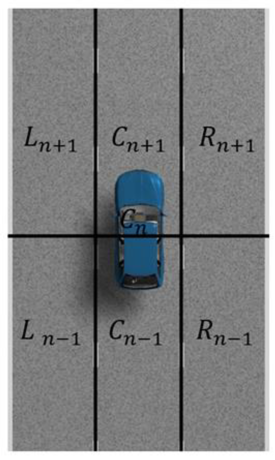
2.1. Vehicle Cluster Environment Analysis

In an actual driving environment, the vehicle motion state can be divided into the free driving state and cluster driving state. The free driving state is when the vehicle is not affected by the surrounding vehicle cluster environment, and the driver is only affected by the free flow speed of the road and can drive freely, according to the driving will. Cluster driving is when the vehicle is constrained by the surrounding cluster vehicles and the vehicle is driven under this constraint. During normal driving, the driver is less willing to drive at a lower than safe target given the influence of self-interested psychology. Based on the driver’s driving needs and the vehicle cluster environment, the driver conducts different driving operations, such as vehicle lane changing and overtaking, to achieve the purpose of quickly traveling on the current road.

2.2. Vehicle Power Demand Forecasting Algorithm in the Vehicle Cluster Environment

The previous section reviewed the driving behavior that the driver may display during the driving process. In this section, the vehicle power demand forecasting algorithm is described for the free-driving and vehicle cluster driving for these driving actions.

The free-flow speed under the traffic flow model has been studied in many publications [11,12,13]. The main factor affecting the free-flow speed is the actual road parameters [14]. In the Highway Capacity Manual, the ideal multi-lane free-flow speed estimation method based on the influence factors of the lane, lane backlash, lane number, and interchange density provided [15] using the following expression:

$$FFS=BFFS-f_{LW}-f_{LC}-f_M-f_A$$

(1)

where $FFS$ is the free-flow speed, BFFS is the base FFS for the multi-lane highway segment, $f_{LW}$ is the adjustment for lane width, $f_{LC}$ is the adjustment for total lateral clearance, $f_M$ is the adjustment for median type, and $f_A$ is the adjustment for access-point density.

In this study, we assumed that the vehicle follows the free-flow speed in the free-running state, and the predicted acceleration ${\frac{d{v}_n\left(t\right)}{dt}}_f$ of the vehicle in the free-running state can be described as:

$${\frac{d{v}_n\left(t\right)}{dt}}_f=\frac{0.278\times FFS-v_n\left(t\right) }{\Delta T}\hspace{1em}\hspace{1em}\hspace{1em}{\frac{d{v}_n\left(t\right)}{dt}}_f\in \left(-a_b{}_{max},a_{max}\right)$$

(2)

where $v_n\left(t\right)$ is the current vehicle speed at time t in meters per second, $a_b{}_{max}$ is the maximum deceleration of the vehicle, and $a_{max}$ is the maximum acceleration of the vehicle.

The vehicle power demand forecast $P_{pre}{}_f$ under free-running conditions can be described as:

$$P_{pre}{}_f=\left(\frac{Gf{u}_a}{3600}+\frac{Gi{u}_a}{3600}+\frac{C_{D}A{u}_a{}^3}{76140}+\frac{\delta m{u}_a}{3600}{\frac{d{v}_n}{dt}}_f\right)$$

(3)

where $G$ is the vehicle gravity, $f$ is the rolling resistance coefficient, $u_a$ is the current vehicle speed in kilometers per hour, $i$ is the gradient, $C_D$ is the coefficient of air resistance, $A$ is the frontal area, $\delta$ is the correction coefficient of rotating mass, and $m$ is the vehicle weight.

Since 1995, Reuschel has used dynamics theory to analyze the traffic flow in vehicle queues and has gradually formed the concept of vehicle following. Many scholars have studied the car-following model [16]. Jin proposed the NLBFVD model based on the full velocity difference model (FVDM) proposed by Jiang et al. in 2010 [17]. The model introduces the lateral separation parameters of the vehicle on the road to consider their influence on the vehicle’s vehicle-pass on the road without lane lines, based on the FVDM model. The differential equation is described as follows:

$$\frac{d{v}_n\left(t\right)}{d}t=k\left\{V\left[\Delta x_{n,n+1}\left(t\right),\Delta x_{n,n+2}\left(t\right)\right]-v_n\left(t\right)\right\}+\lambda G\left(\Delta v_{n,n+1}\left(t\right),\Delta v_{n,n+2}\left(t\right)\right)$$

(4)

where $k$ is the driver’s sensitivity factor for the difference between the best speed and the current speed, which is 0.41; $\lambda$ is the sensitivity coefficient of the response to the stimulus $G(·)$, which is 0.8$; \Delta x_{n,n+1}\left(t\right)\equiv x_{n+1}\left(t\right)-x_n\left(t\right)$ is the distance headway between the vehicle n and the vehicle in front n + 1 at time t; $\Delta x_{n,n+2}\left(t\right)\equiv x_{n+2}\left(t\right)-x_n\left(t\right)$ is the distance headway between the vehicle n and the front vehicle n + 2 at time t; $\Delta v_{n,n+1}\left(t\right)\equiv v_{n+1}\left(t\right)-v_n\left(t\right)$ is the speed difference between vehicle n and front vehicle n + 1 at time t; and $\Delta v_{n,n+2}\left(t\right)\equiv v_{n+2}\left(t\right)-v_n\left(t\right)$ is the speed difference between vehicle n and front vehicle n + 2 at time t.

The functions $V\left[\Delta x_{n,n+1}\left(t\right),\Delta x_{n,n+2}\left(t\right)\right]$ and $G\left(\Delta v_{n,n+1}\left(t\right),\Delta v_{n,n+2}\left(t\right)\right)$ mean the following:

$$V\left[\Delta x_{n,n+1}\left(t\right),\Delta x_{n,n+2}\left(t\right)\right]=V\left[\left(1-p_n\right)\Delta x_{n,n+1}\left(t\right)+p_n\Delta x_{n,n+2}\left(t\right)\right]$$

(5)

$$V\left[\Delta x_{n,n+1}\left(t\right),\Delta x_{n,n+2}\left(t\right)\right]=V\left[\left(1-p_n\right)\Delta x_{n,n+1}\left(t\right)+p_n\Delta x_{n,n+2}\left(t\right)\right]$$

(6)

$$V\left[\Delta x\right]=0.5v_{max}\left[tanh\left(\Delta x-h_c\right)+tanh\left(h_c\right)\right]$$

(7)

where $V(·)$ is the speed optimization function proposed by Bando et al. [18]; $h_c$ is the safe distance between vehicle n and the front vehicle, which is 5 m; $p_n=L{S}_n/L{S}_{max}$ is the lateral separation distance influence parameter; $L{S}_n$ is the lateral separation distance between vehicle n and front vehicle $n+1$; $L{S}_{max}$ is the maximum lateral separation distance, which is generally 3.6 m; and $p_n$ is the description of the degree of lateral separation between the following vehicle and the preceding vehicle. When the value reaches the maximum, the following vehicle and the preceding vehicle are already in two different lanes, and the following vehicle has completed the lane changing operation. Later, He [19] introduced the lateral overtaking stimulation parameters, and Zhang [20] introduced the longitudinal overtaking stimulation parameters, to supplement the NLBFVD model. However, when the driver is driving in a real vehicle cluster state, it is necessary to consider not only the lateral separation between the following vehicle and the preceding vehicle, but also the overall state of the adjacent vehicles in each lane. In this regard, this paper introduces random utility theory to conduct an in-depth study of the NLBFVD model, and proposes a three-lane vehicle-following model considering the vehicle cluster environment.

This model selects six vehicles around the vehicle under study to form a vehicle cluster environment. The cluster environment information includes the driving state and position relationship of each vehicle. The effect of the vehicles in each lane on the following behavior of the following vehicle in the cluster environment is expressed in this model as the utility value of the lane to the vehicle under study. Figure 2 shows a schematic diagram of a three-lane vehicle-following model cluster environment.

Here, $C_n$ is the current vehicle, $L_{n+1}$ is the front vehicle on the left road, $L_{n-1}$ is the rear vehicle on the left road, $C_{n+1}$ is the front vehicle on the current road, $C_{n-1}$ is the rear vehicle on the current road, $R_{n+1}$ is the front vehicle on the right road, and $R_{n-1}$ is the rear vehicle on the right road.

The three-lane car following model in a cluster environment can be expressed as:

$$\begin{array}{c}{\frac{d{v}_{Cn}\left(t\right)}{dt}}_c=\alpha \left\{V\left[\Delta x_{L_{n+1},C_n}\left(t\right),\Delta x_{C_{n+1.},C_n}\left(t\right),\Delta x_{R_{n+1},C_n}\left(t\right)\right]-v_{C_n}\left(t\right)\right\}\\ \hspace{1em}\hspace{1em}\hspace{1em}\hspace{1em}+kG\left[\Delta v_{L_{n+1},C_n}\left(t\right),\Delta v_{C_{n+1.},C_n}\left(t\right),\Delta v_{R_{n+1},C_n}\left(t\right)\right]\end{array}$$

(8)

where $v_{C_n}\left(t\right)$ is the velocity of vehicle n at time t, $\Delta x_{L_{n+1},C_n}\left(t\right)\equiv x_{L_{n+1}}\left(t\right)-x_{C_n}\left(t\right)$ is the distance between the vehicle $L_{n+1}$ and the vehicle $C_n$ at time t, $\Delta x_{C_{n+1},C_n}\left(t\right)\equiv x_{C_{n+1}}\left(t\right)-x_{C_n}\left(t\right)$ is the distance between the vehicle $C_{n+1}$ and the vehicle $C_n$ at time t, $\Delta x_{R_{n+1},C_n}\left(t\right)\equiv x_{R_{n+1}}\left(t\right)-x_{C_n}\left(t\right)$ is the distance between the vehicle ${\mathrm{R}}_{\mathrm{n}+1}$ and the vehicle $C_n$ at time t, $\Delta v_{L_{n+1},C_n}\left(t\right)\equiv v_{C_n}\left(t\right)-v_{L_{n+1}}\left(t\right)$ is the speed difference between the vehicle $C_n$ and the vehicle $L_{n+1}$ at time t, $\Delta v_{C_{n+1},C_n}\left(t\right)\equiv v_{C_n}\left(t\right)-v_{C_{n+1}}\left(t\right)$ is the speed difference between the vehicle $C_n$ and the vehicle $C_{n+1}$ at time t, and $\Delta v_{R_{n+1},C_n}\left(t\right)\equiv v_{C_n}\left(t\right)-v_{R_{n+1}}\left(t\right)$ is the speed difference between the vehicle $C_n$ and the vehicle $R_{n+1}$ at time t. The functions $V(·)$ and $G(·)$ mean the following:

$$V\left[\Delta x_{L_{n+1},C_n}\left(t\right),\Delta x_{C_{n+1.},C_n}\left(t\right),\Delta x_{R_{n+1},C_n}\left(t\right)\right]=V\left[P_{L,C_n}\Delta x_{L_{n+1},C_n}\left(t\right)+P_{C,C_n}\Delta x_{C_{n+1.},C_n}\left(t\right)+P_{R,C_n}\Delta x_{R_{n+1},C_n}\left(t\right)\right]$$

(9)

$$G\left[\Delta v_{L_{n+1},C_n}\left(t\right),\Delta v_{C_{n+1.},C_n}\left(t\right),\Delta v_{R_{n+1},C_n}\left(t\right)\right]=G\left[P_{L,C_n}\Delta v_{L_{n+1},C_n}\left(t\right)+P_{C,C_n}\Delta v_{C_{n+1.},C_n}\left(t\right)+P_{R,C_n}\Delta v_{R_{n+1},C_n}\left(t\right)\right]$$

(10)

where $P_L$, $P_C$, and $P_R$ are the probability that the vehicle $C_n$ selects the left road, the current road, and the right road, respectively, according to the random utility theory, as follows:

$$P_{i,C_n}=Prob\left[V_{C_n,i}>V_{C_n,k}\right]\hspace{1em}k\ne i$$

(11)

where ${\mathrm{V}}_{\mathrm{C}n,i}$ is the total utility of lane $i$ to vehicle $C_n$ and $V_{Cn,k}$ is the total effect of other lanes on vehicle $C_n$.

The total utility is calculated as:

$$V_{C_n,i}=U_{C_n,i}+{\epsilon }_{C_n,i}={\beta }_0+{\displaystyle \sum }_{j=1}^N{\beta }_j{X}_{C_n,i,j}+{\epsilon }_{C_n,i}$$

(12)

where $U_{C_n,i}$ is the fixed utility of lane $i$ to vehicle C_n, ${\epsilon }_{C_n,i}$ is the unfixed utility of lane $i$ to vehicle $C_n$, $X_{C_n,i,j}$ is the jth variable that affects the fixed utility of vehicle $C_n, {\beta }_0$ is a constant, and ${\beta }_j$ is a coefficient. Since the double exponential distribution function is similar to the normal distribution and the double exponential distribution function has a higher enforceability than the normal distribution function, assuming that ε obeys the double exponential distribution, the following logit model can be obtained:

$$P_{i,C_n}=\frac{e^{U_{C_n,i}}}{{{\displaystyle \sum }}_{k\in A}{e}^{U_{C_n,k}}}iϵA$$

(13)

The power demand forecast for the vehicle-to-powertrain in a cluster environment can be derived from the vehicle power balance equation as follows:

$$P_{pre}{}_c=\left(\frac{Gf{u}_a}{3600}+\frac{Gi{u}_a}{3600}+\frac{C_{D}A{u}_a{}^3}{76140}+\frac{\delta m{u}_a}{3600}{\frac{d{v}_n\left(t\right)}{dt}}_c\right)$$

(14)

Combined with Equation (3), the demand power prediction can be described as:

$$P_{pre}=\{\begin{array}{l}\left(\frac{Gf{u}_a}{3600}+\frac{Gi{u}_a}{3600}+\frac{C_{D}A{u}_a{}^3}{76140}+\frac{\delta m{u}_a}{3600}{\frac{d{v}_n\left(t\right)}{dt}}_f\right) TH\ge 5\\ \left(\frac{Gf{u}_a}{3600}+\frac{Gi{u}_a}{3600}+\frac{C_{D}A{u}_a{}^3}{76140}+\frac{\delta m{u}_a}{3600}{\frac{d{v}_n\left(t\right)}{dt}}_c\right) TH<5\end{array}$$

(15)

where TH is the time headway in the Highway Capacity Manual Third Edition that defines whether the vehicle is in the car-following state [21].

3. Vehicle Model

The electric vehicle model equipped with EMCVT is described in this section.

3.1. Vehicle Parameters

The vehicle parameters are as follows: the whole vehicle has a mass of 1470 kg, the wheel radius is 0.314 m, the maximum output power of the motor is 38 kW, the maximum torque of the motor is 120 N·m, and the range of the EMCVT transmission ratio $i_0$ is 0.5 to 2.0. The main reduction ratio $i_g$ is 6.

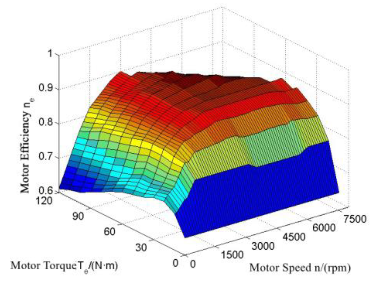
3.2. Motor Efficiency Model

The motor efficiency model is based on motor bench test data. Figure 3 shows the motor efficiency model.

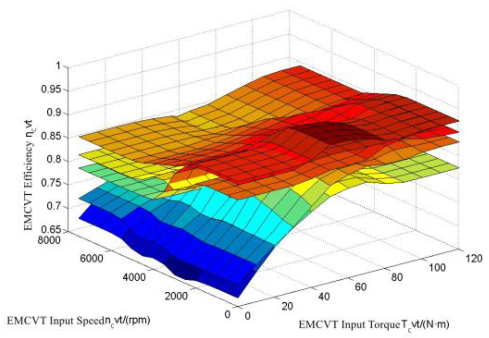
3.3. EMCVT Efficiency Model

The efficiency of the continuously variable transmission is mainly determined by the input speed, input torque, and transmission ratio. The EMCVT efficiency model was established using the test data. Figure 4 shows the EMCVT efficiency model.

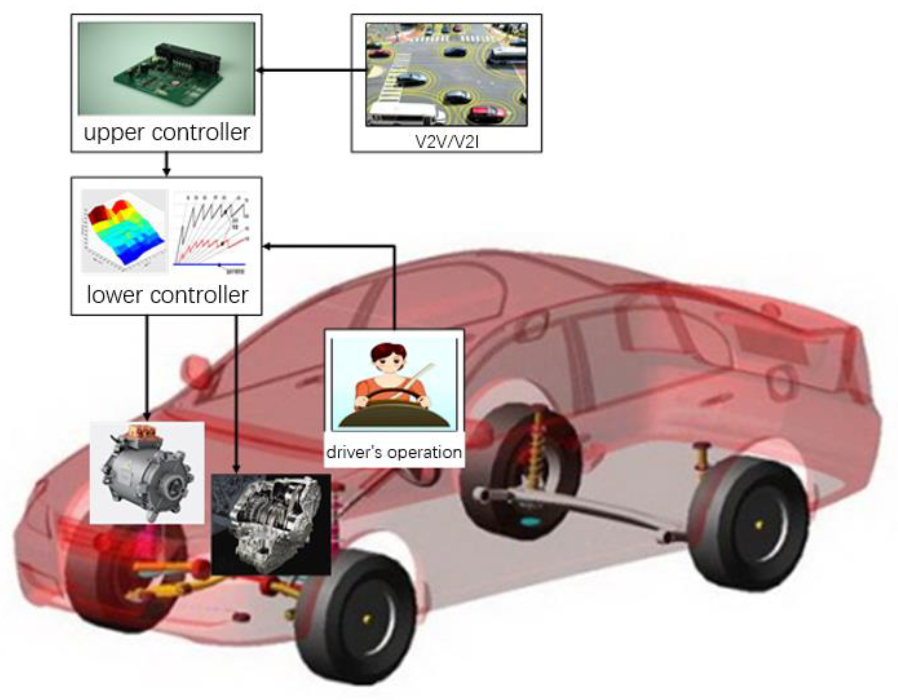
4. Research on the Active Control Strategy of the Powertrain System

In Section 2, the vehicle demand power prediction algorithm was proposed. This section explains the control strategy of the vehicle powertrain based on the characteristics of the vehicle powertrain system.

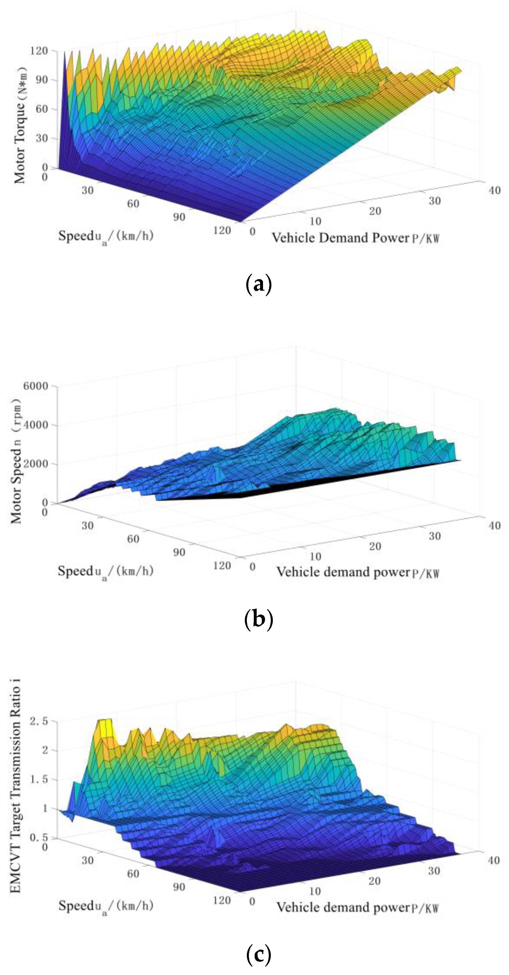
4.1. Optimal Working Point Calculation for the Vehicle Powertrain System

In the calculation process of the vehicle powertrain working state, we selected the accelerator pedal opening degree and the vehicle speed to show the current vehicle driving condition, and to comprehensively consider the vehicle power and economy to calculate the working state of the vehicle powertrain. The control problem in this case can be described as an optimization problem: looking for the best powertrain operating point for a given vehicle speed and driver’s accelerator pedal operation, and considering the vehicle’s economy and power.

The system optimization objective function is the maximum evaluation function max $p$, which can be expressed as

$$Powe{r}_e=Moto{r}_e\times CV{T}_e$$

(16)

$$a=\frac{F_t-F_f-F_i-F_w}{\delta m}$$

(17)

$$p=\gamma nor\left(Powe{r}_e\right)+\delta nor\left(a\right)$$

(18)

where $Powe{r}_e$ is the vehicle powertrain efficiency, $Moto{r}_e$ is the motor efficiency, $CV{T}_e$ is the EMCVT efficiency, $a$ is the vehicle acceleration, $F_t$ is the driving force, $F_f$ is the rolling resistance, $F_i$ is the slope resistance, $F_w$ is the air resistance, $\delta$ is the rotation mass conversion factor, $p$ is the valuation function in the driving state, and $\gamma$ and $\delta$ are the weighting coefficients.

Coupling exists between the economy and power of the car and the efficiency of the vehicle’s powertrain and the actual output torque. In this paper, through forward calculation, the heuristic search algorithm is used to solve the EMCVT target transmission ratio considering economic and dynamic parameters.

At present, drive control strategies for pure electric vehicles mainly fall into three categories, as shown in Figure 5.

Curve 1 represents a radical driving control strategy, which is mostly used for vehicle sports mode. Curve 3 represents a mild driving control strategy, which is mostly used for the snow mode of vehicles. In practical applications, the driving control strategies curve is generally between curves 1 and 3. In order to simplify the model and express it more intuitively, line 2 is used in this paper to express the relationship between accelerator pedal opening and motor output torque. The best working point solving process is shown in Figure 4. The overall solution idea is as follows: (1) The acceleration pedal opening range is set from 0 to 1, with Δ$A$ as the step length; (2) the speed range is set from 0 to 120 km/h, with Δ$v$ as the step length; (3) all acceleration pedal step and vehicle speed step combinations are traversed. In each combination, the EMCVT transmission ratio varies in the range of 0.5 to 2.0, with Δ$i$ being the step size. The total vehicle power efficiency and vehicle acceleration under different EMCVT transmission ratios are calculated, and the total vehicle power efficiency and vehicle acceleration under different transmission ratios are normalized; (4) and the motor output torque, motor output speed, and EMCVT transmission ratio corresponding to the maximum estimation function are taken as the working points of the power assembly under the current acceleration pedal opening and vehicle speed. Figure 6 shows the powertrain working point calculation process.

The calculation results for Δ$A=0.02,$ Δ$v=2,$ and Δ$i=0.01$ are provided in Figure 7.

The target transmission ratio of the EMCVT is determined by the target speed and target torque of the motor to ensure that the powertrain system works at the optimal operating point under ideal conditions.

4.2. Vehicle Powertrain System Active Control Strategy

Active control is more forward-looking than passive control. Active control of the optimal working point of the vehicle powertrain under different working conditions is an active choice of changing the path of the working point of the vehicle powertrain from the current working condition to the next working condition. During control of the vehicle powertrain system operating point, the operating point torque is mainly determined by the motor torque control, and the operating point speed is mainly achieved by the transmission adjusting transmission ratio. Therefore, this strategy mainly includes two modules: the EMCVT target transmission ratio algorithm module and the motor torque compensation module.

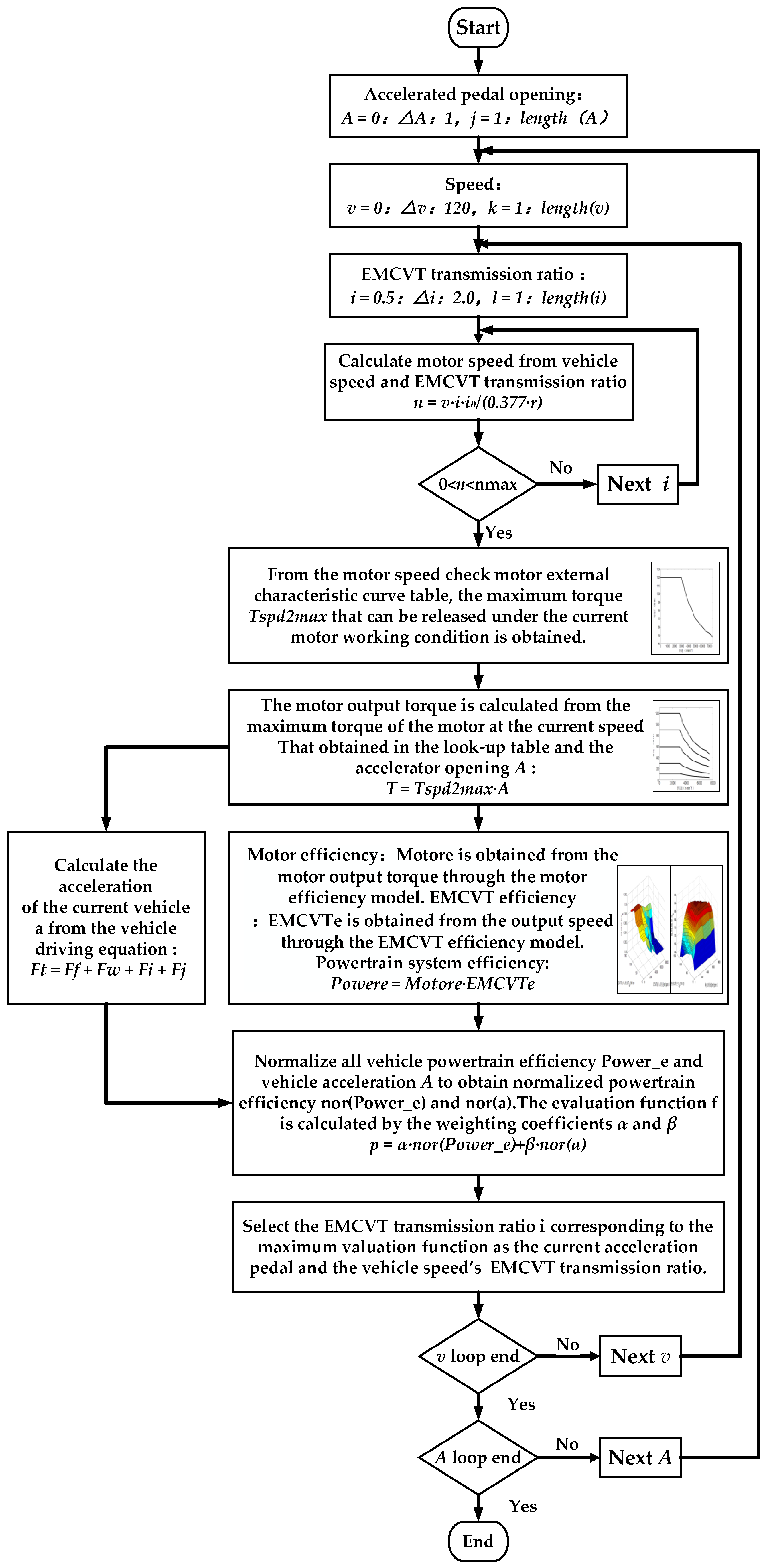
4.2.1. EMCVT Target Transmission Ratio Solving Model

According to the motion prediction of the vehicle in the cluster environment and the driver’s driving intention, the vehicle motion state can be predicted at the next moment, the EMCVT transmission ratio is actively adjusted, and the vehicle powertrain system is actively controlled. The EMCVT target transmission ratio solution model obtained by predicting the required power of the vehicle powertrain is:

$$P_c=\tau \left(P_{pre}-P_{rt}\right)$$

(19)

$$P_{obj}=P_{rt}+P_c$$

(20)

$$P_{M_{obj}}=\frac{P_{obj}}{CV{T}_e}$$

(21)

$$A_{pre}=f\left(P_{M_{obj}}\right)$$

(22)

$$CV{T}_i{}_{obj}=g\left(A_{pre},u_a\right)$$

(23)

where $P_c$ is the vehicle powertrain compensation power, $P_{rt}$ is the current output power of the vehicle powertrain, $\tau$ is the compensation power factor, $P_{obj}$ is the target power output of the vehicle powertrain, $P_{M_{obj}}$ is the motor target output power, $f(·)$ is the motor output power–accelerator pedal opening relationship model, and $g(·)$ is the acceleration pedal opening degree-vehicle speed–EMCVT transmission ratio relationship model. The compensation power coefficient $\tau$ is calculated using a fuzzy control algorithm. The input variables of the fuzzy controller are the expected acceleration $\frac{d{v}_n\left(t\right)}{dt}$ and the accelerator opening change rate A, and the output variable is the power compensation coefficient $\tau$. The linguistic variables of the expected acceleration are NV, NB, NM, NS, ZO, PS, PM, PB, and PV, and the universe is −5 to 3. The linguistic variables of the change rate for the accelerator pedal opening are NM, NS, ZO, PS, and PM, and the universe is −1 to 1. The linguistic variables of the power compensation coefficient are NV, NB, NM, NS, ZO, PS, PM, PB, and PV, and the universe is −1 to 1. NV, NB, NM, NS, ZO, PS, PM, PB, and PV correspond respectively Negative Very Big, Negative Big, Negative Middle, Negative Small, Zero, Positive Small, Positive Middle, Positive Big, Positive Very Big. Express different degrees in fuzzy control. Figure 8 shows the membership function of the input variable and the output variable of the fuzzy control algorithm.

Table 1. The fuzzy rule description.

Expected Acceleration	Change Rate for The Accelerator Pedal Opening
	NM	NS	ZO	PS	PM
NV	NV	NV	NB	ZO	ZO
NB	NB	NB	NM	ZO	ZO
NM	NM	NM	NS	ZO	ZO
NS	NM	NS	NS	ZO	ZO
ZO	NM	NS	NS	ZO	ZO
PS	ZO	ZO	ZO	PS	PS
PM	ZO	ZO	PS	PM	PM
PB	ZO	ZO	PM	PB	PB
PV	ZO	ZO	PB	PV	PV

describes the fuzzy rule. Figure 9 shows the transfer function obtained by the fuzzy algorithm.

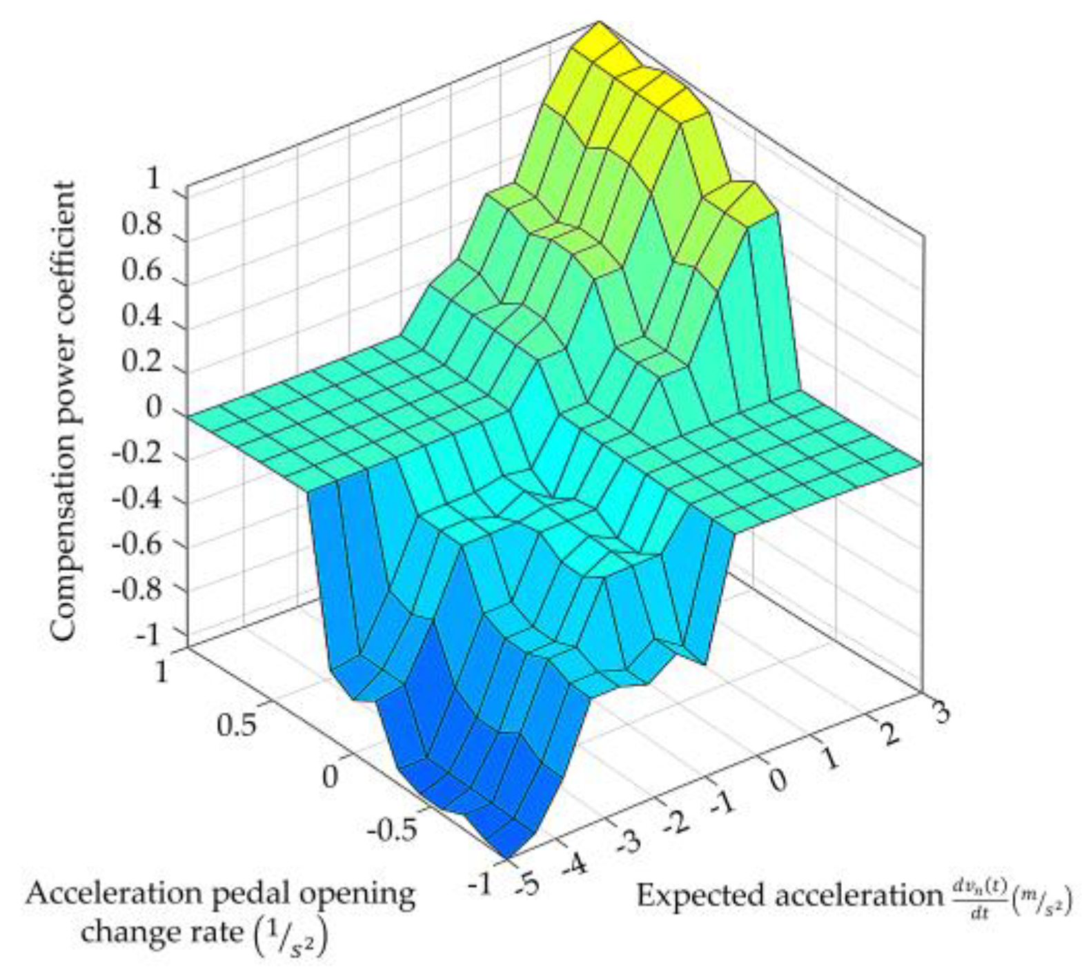
4.2.2. Motor Torque Compensation

In the process of EMCVT active speed regulation, to maintain the stability of the longitudinal motion of the vehicle and follow the driver’s driving intention, torque compensation of the motor torque is required. The algorithm compensates for the passive control target torque of the motor according to the compensation power, and outputs the active control torque. Figure 10 shows the torque compensation algorithm.

4.2.3. Vehicle Torque Control System Passive Control Target Torque Calculation

The passive control output torque refers to the torque output by the motor according to the passive control strategy without the backup power prediction, and is related to the accelerator opening and vehicle speed. The functional relationships are as follows:

$$P_{M_{def}}=f^{-1}\left(A\right)$$

(24)

$$CV{T}_i{}_{obj}=g\left(A,u_a\right)$$

(25)

$$n=\frac{u_a\times CV{T}_i\times i_g}{0.377\times r}$$

(26)

$$T_{def}=\frac{9550\times P_{M_{def}}}{0.377}$$

(27)

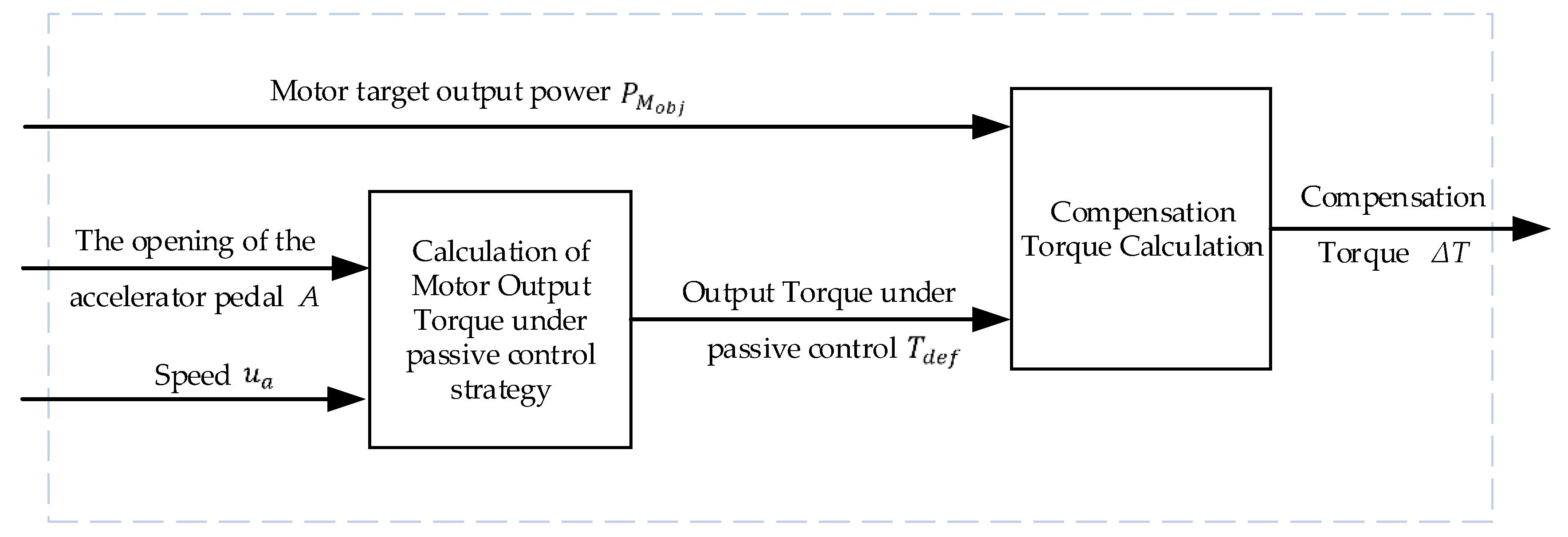
4.2.4. Compensation Torque Calculation

The compensation torque is used to compensate for the motor output torque under the condition of actively controlling the EMCVT transmission ratio, which is related to the target output power $P_{obj}$ of the powertrain vehicle powertrain. Its function expressions are as follows:

$$T_{M_{obj}}=\frac{9550\times P_{M_{obj}}}{0.377}$$

(28)

$$\Delta T=T_{M_{obj}}-T_{def}$$

(29)

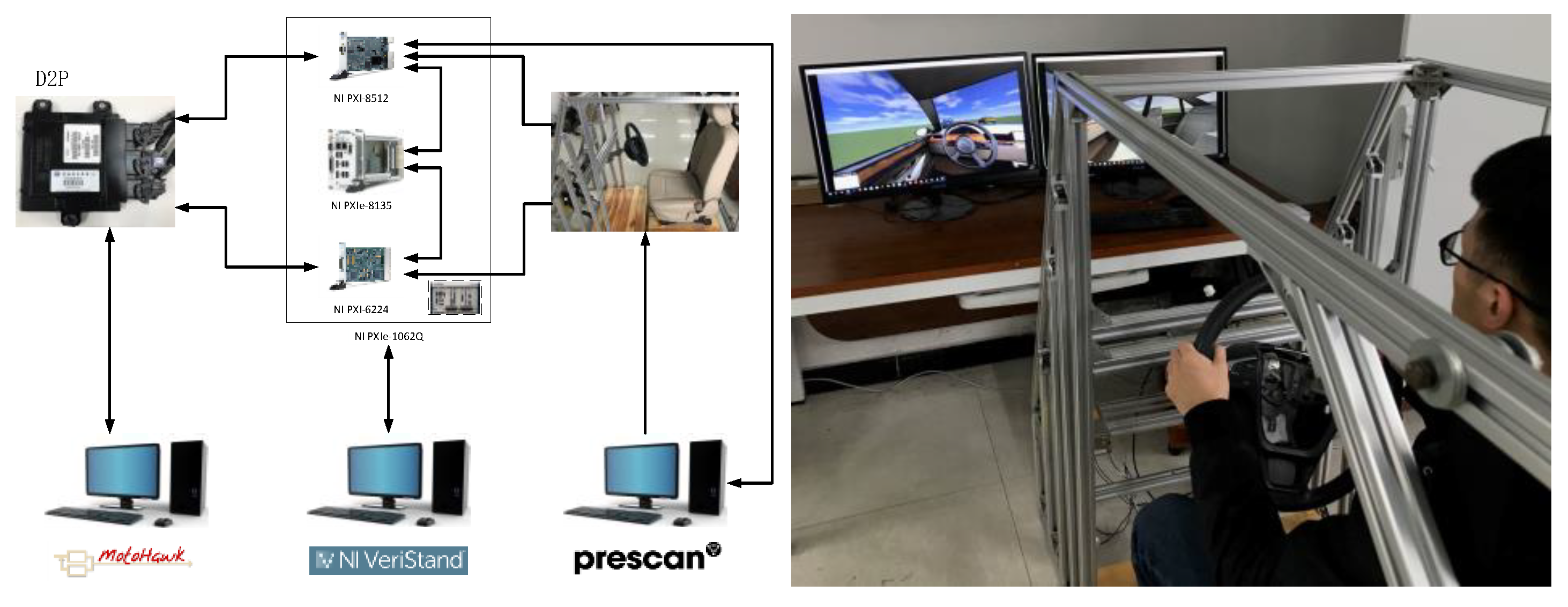
5. Test Environment Construction and Test Examples

To verify the effectiveness of the optimization strategy, based on the NI-PXI system (National Instruments, Austin, TX, USA), we built a driver-in-the-loop hardware-in-the-loop (HIL) test platform based on real traffic scenarios, as shown in Figure 11. Based on a field trip to the real road, and the acquisition of accurate road information from OpenStreetMap, the test environment was built using Prescan (Tass International, Helmond, The Netherlands). In this test platform, drivers sense the environment by watching the screen of a computer equipped with Prescan, and operate the accelerator pedal, brake pedal, and steering wheel in the cockpit. The NI-PXI system collects Prescan information and the cockpit signal, and communicates with the Vehicle Control Unit (VCU) and Prescan. The computer equipped with MotoHawk can write and calibrate VCU software. The computer equipped with NI Veristand can deploy the vehicle model to the NI PXIe system.

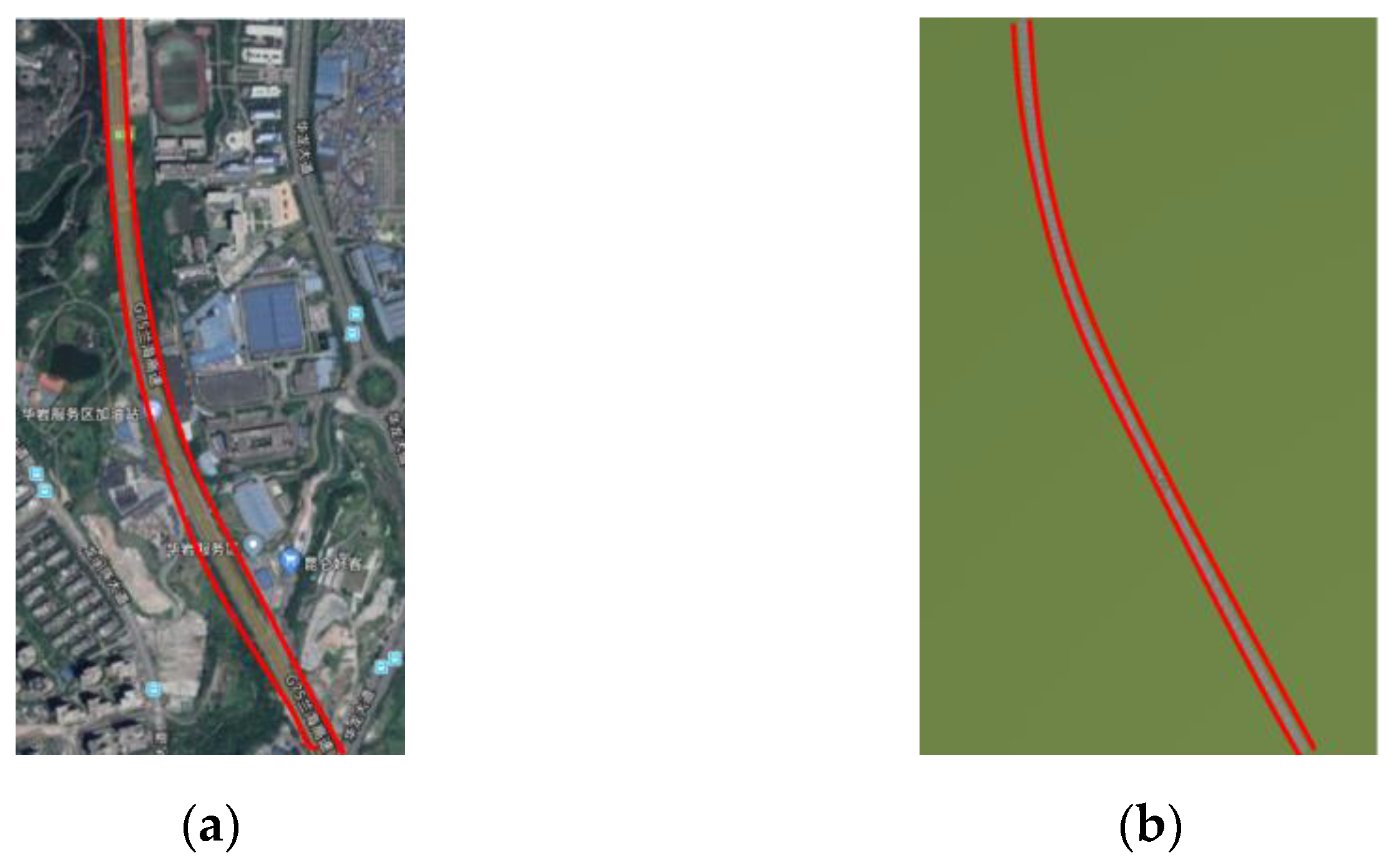
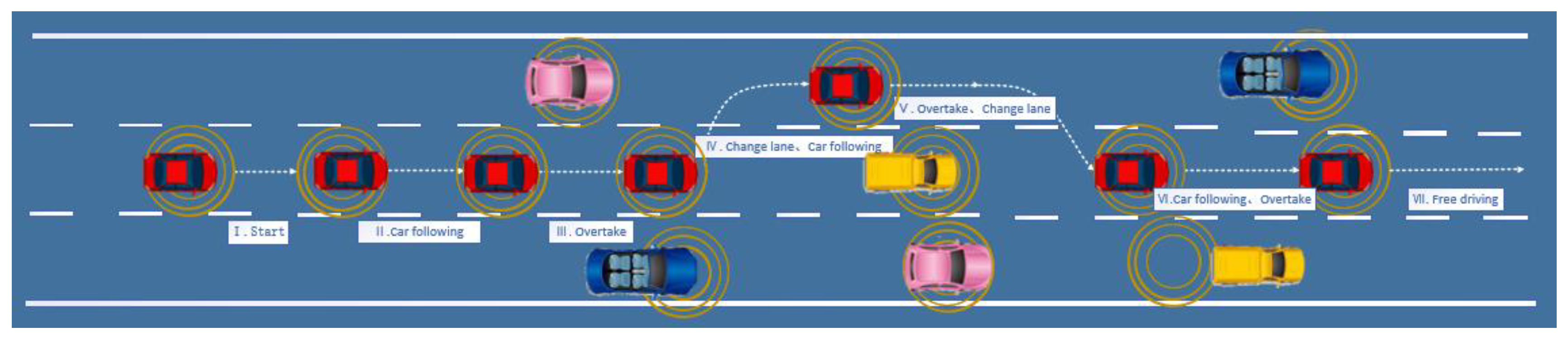
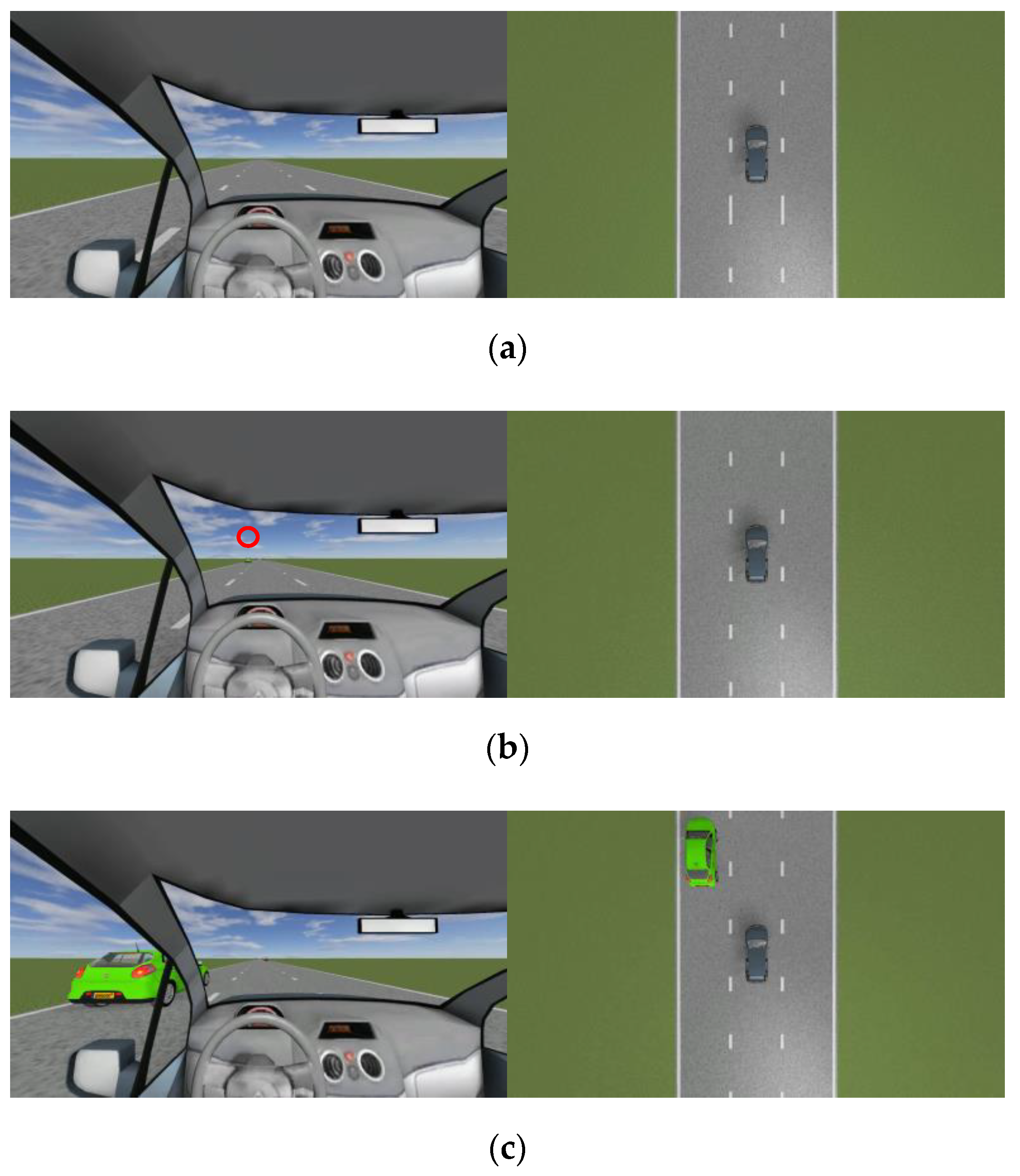
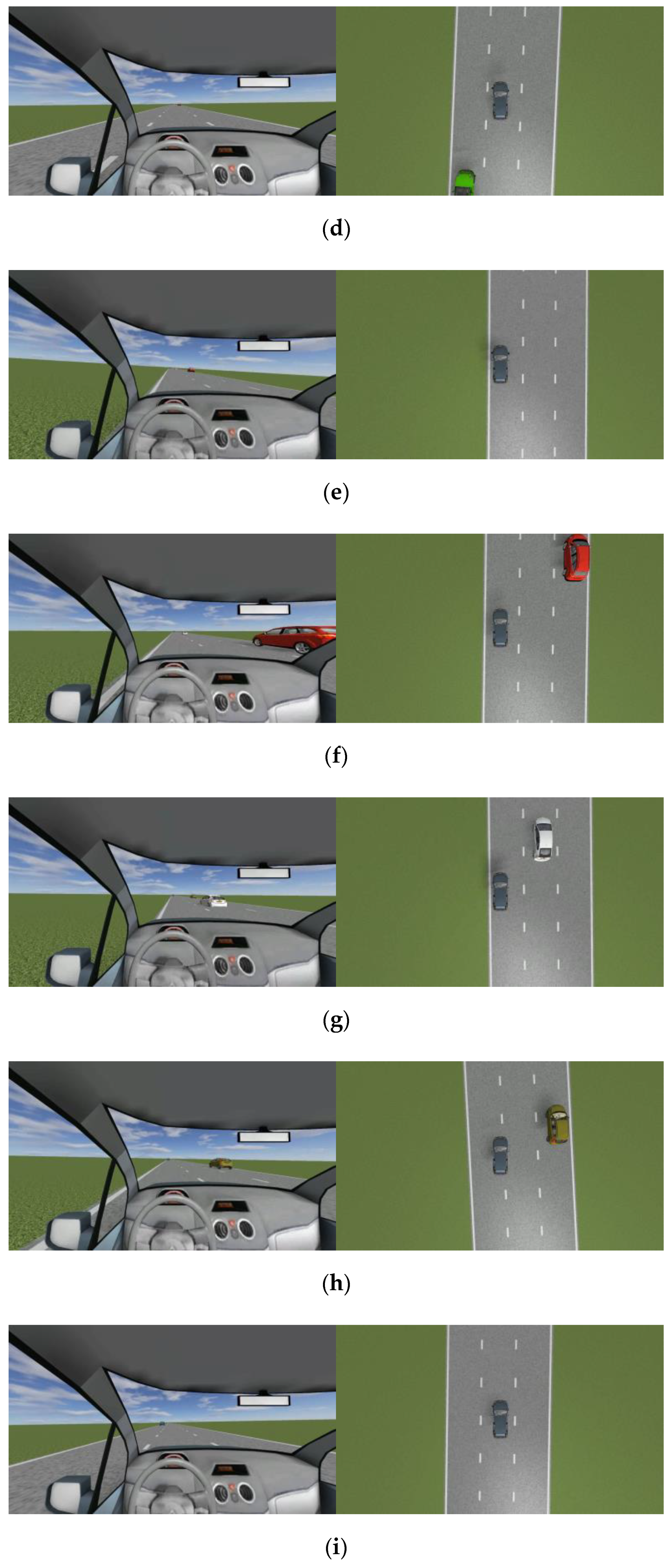
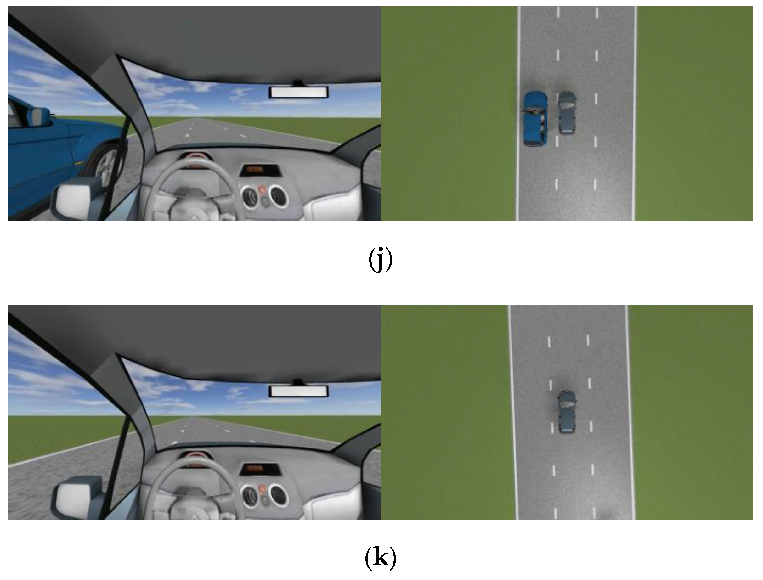
5.1. Traffic Scene Construction

We selected the G75 Lanhai Expressway Inner Ring Expressway from Banan to Yubei Road in the Jiulongpo District of Chongqing City, China, as the research object to model a traffic scene. Figure 12a shows a high-precision map of the road that was studied. The road is a two-way, six-lane road, with a maximum speed of 100 km/h. The test section selected in this paper is about 1280 m. In this study, we did not consider the traffic light signal, branch road, weather, or road surface. Figure 12b shows the virtual traffic road scene, as displayed by Prescan.

5.2. Test Process Design

Based on the actual driving process, the test process can be divided into seven stages: (1) The vehicle starts from a standstill; (2) the vehicle enters the car-following state as it is affected by the preceding vehicle; (3) the vehicle overtakes a vehicle on the left; (4) the vehicle drives into the left lane, and enters the car-following state under the influence of the front car; (5) the vehicle overtakes on the right side of the vehicle; (6) the vehicle enters the right lane, and enters the car-following state under the influence of the front car; and (7) the vehicle exits the cluster environment, and enters free driving. Figure 13 shows the test process decomposition.

The vehicle under test and other vehicles in the cluster environment have GPS positioning and vehicle–vehicle and vehicle–road communication capabilities, and the data transmission is correct and without delay. All vehicles except for the vehicle under study are set to run at a constant speed.

6. Test Results and Analysis

According to the solution in this paper, a hardware-in-the-loop test platform based on the human driver and Vehicle Control Unit (VCU) in-loop was built. Through this platform, we tested the proposed strategy.

The human driver controls the vehicle under test, the driver’s operation signal and the vehicle powertrain system state parameters are collected by the NI-PXI system, and the passive and active control strategies are tested simultaneously. Figure 14 shows the positional relationship between the tested vehicle and the cluster environment during the test. Figure 15 shows the test result curve, where the solid line is the active control strategy test result and the dashed line is the passive control strategy test result. Figure 14 and Figure 15a show that during phases I, II, III, V, and VI, the driver has a continuous acceleration demand, and the vehicle powertrain system needs to provide considerable backup power. In stage IV, the driver drives gently, and in stage VII, the vehicle drives out of the cluster environment and the speed is close to the designed road speed. In phases IV and VII, the vehicle has a lower demand for backup power. Figure 14b shows that in the I, II, and III phases, when the vehicle speed is increasing, the EMCVT transmission ratio under the active control strategy control maintains a larger target gear ratio than the passive control strategy. The goal is to provide sufficient backup power for the vehicle. In the fourth stage, the distance between the vehicle being tested and the preceding vehicle is continuously reduced, the upper controller predicts that the demand power is decreasing, and the EMCVT target transmission ratio under the active control strategy is continuously approaching the passive control EMCVT target transmission ratio. In stages V and VII, the predicted backup power is zero, so the active control of EMCVT is the same as the passive control transmission ratio. Figure 15c shows the EMCVT real output transmission ratio. Under the active control strategy, EMCVT can be properly controlled and corresponds in time. Figure 15d, Figure 15e, and Figure 15f respectively show the efficiency of EMCVT, the motor, and the vehicle powertrain system in the test process, providing data for the conclusion of this paper. Figure 16 shows the EMCVT output transmission ratio change rate for two control strategies. Figure 16 shows that the maximum peak value, the peak number, and the average rate of change in the EMCVT output transmission ratio under the control of the active control strategy are better than with passive control. According to the calculation, compared with the passive control strategy, the EMCVT output transmission ratio change rate for the active control strategy is reduced by 33.38%, the average change rate is reduced by 42.57%, and the motor efficiency is increased by 0.61%. Figure 17 shows the vehicle powertrain system and component part’s efficiency difference diagram. The difference shown in the figure is the efficiency under the active control strategy minus the efficiency under the control of the passive control strategy. Figure 17 shows that although the overall efficiency of EMCVT has decreased, the efficiency of the motor has significantly increased. This means that the overall efficiency of the vehicle powertrain system under the control of the active control strategy is better than under the passive control strategy. When using the active control strategy, the overall efficiency of the vehicle powertrain system is increased by 0.6% compared to the passive control strategy.

7. Conclusions

An active control strategy for the EV based on the vehicle cluster environment is proposed. The effectiveness of the proposed strategy is validated via the simulation, which reduces the working intensity of EMCVT and improves the efficiency of the transmission system assembly of the EV. The following work was conducted in this study:

• In this study, according to the driving characteristics of a vehicle, the driving demand of a vehicle in a cluster environment was analyzed, and the dynamic prediction algorithm based on the car-following model of the cluster environment was proposed;
• Based on the forward calculation algorithm, passive control of the vehicle powertrain system was solved. Based on passive control, the vehicle power demand forecast, the driver’s driving operation, an active control strategy for the vehicle powertrain system was designed;
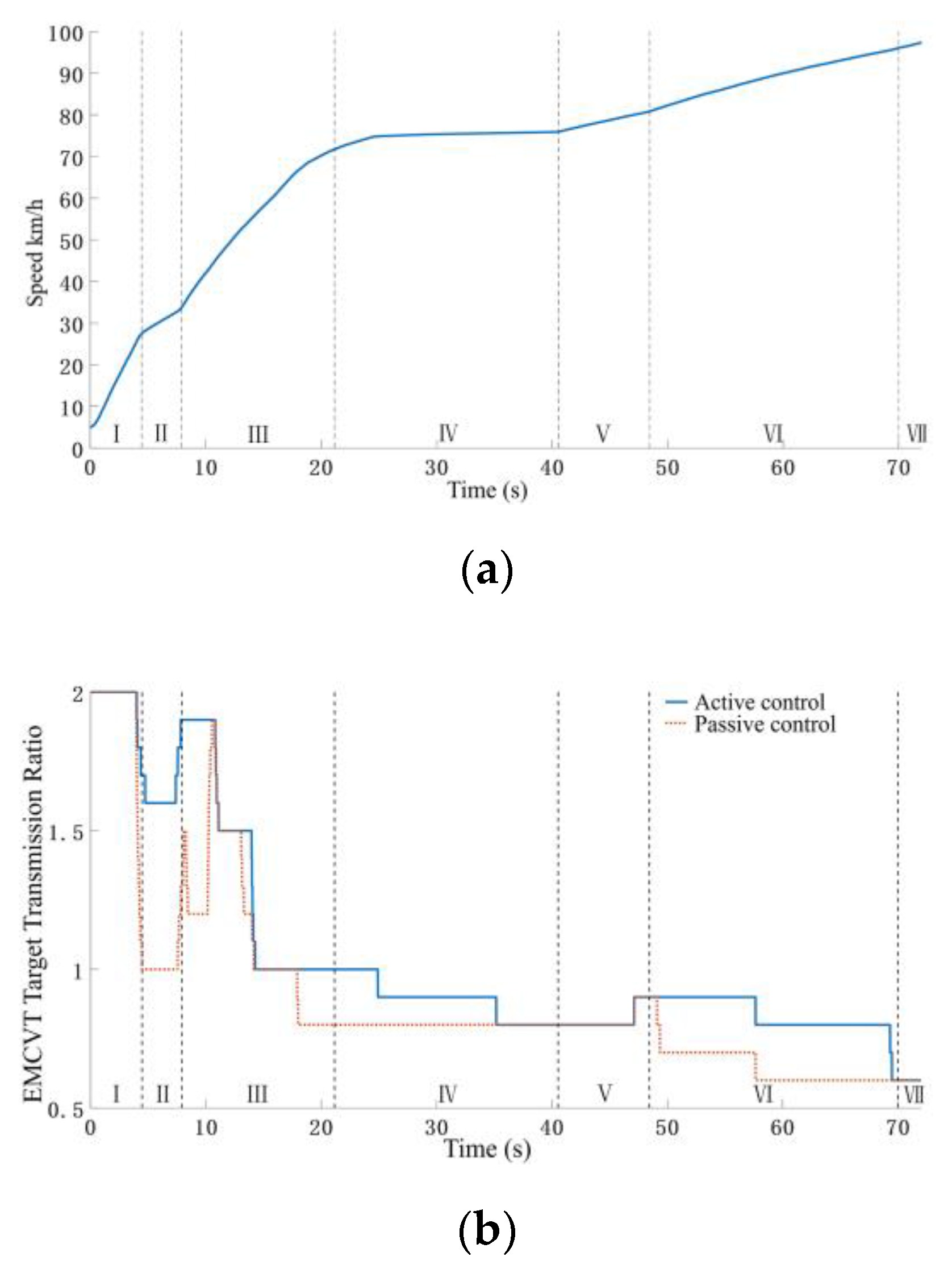
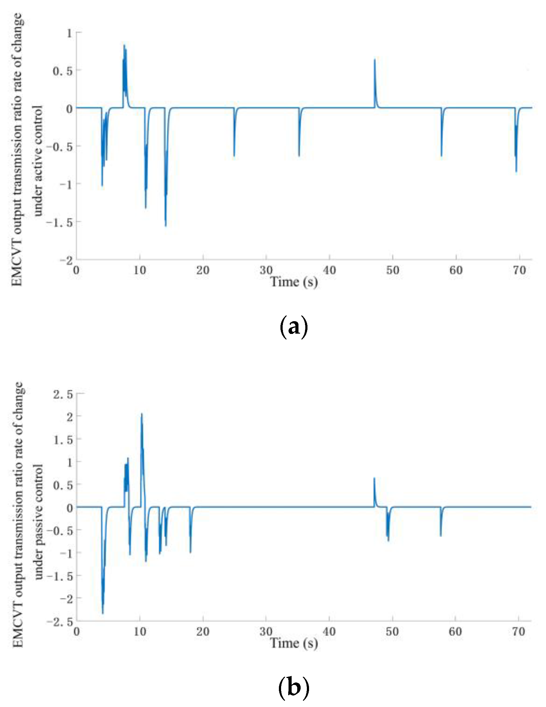
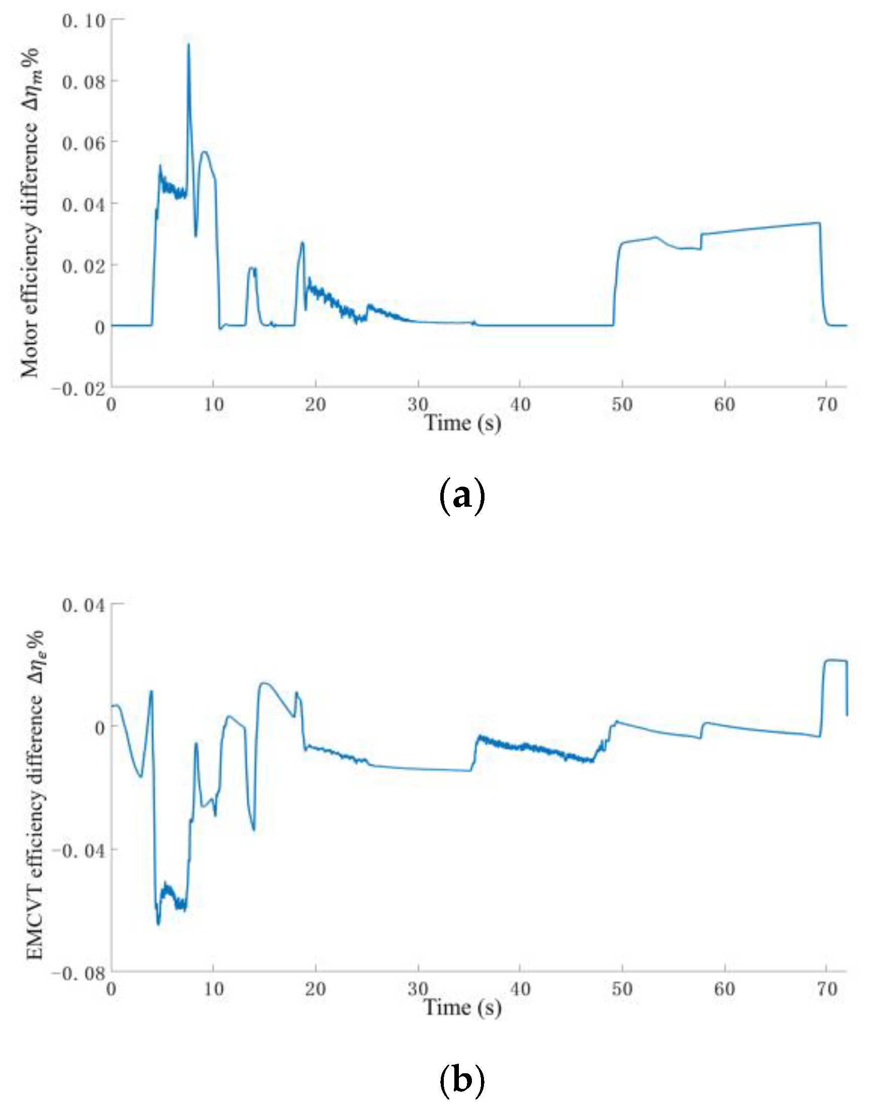
• The control strategy was tested based on the driver’s real-time test platform. The test data showed that under the same hardware conditions, the vehicle powertrain under the control of the active control strategy can effectively and quickly provide backup power compared with the passive control strategy. Compared with passive control, under the active control strategy, the motor efficiency increased by 0.61%, the EMCVT transmission ratio average rate of change reduced by 42.57%, and the overall efficiency of the vehicle powertrain system increased by 0.6%.

Although this paper proposes an active control strategy based on a vehicle cluster environment, this method is more precise for flat highways with fewer vehicles. Our next step will focus on extending the strategy application for different traffic environments, including rush hours, and different vehicle driving cycles, including braking energy recovery.

References

1. Yu, Z.; Guo, G. Coordinated Path Following Control of Vehicle Formations in Vehicular Network Environment. Control Eng. China 2015, 5, 804–808. [Google Scholar]
2. Cerna, F.V.; Pourakbari-Kasmaei, M.; Contreras, J.; Gallego, L.A. Optimal Selection of Navigation Modes of HEVs Considering CO 2 Emissions Reduction. IEEE Trans. Veh. Technol. 2019, 68, 2196–2206. [Google Scholar] [CrossRef]
3. Ma, Y.; Huang, J.; Zhao, H. Method of vehicle formation control based on Vehicle to Vehicle communication. J. Jilin Univ. (Eng. Technol. Ed.) 2018. [Google Scholar] [CrossRef]
4. Tribioli, L. Energy-Based Design of Powertrain for a Re-Engineered Post-Transmission Hybrid Electric Vehicle. Energies 2017, 10, 918. [Google Scholar] [CrossRef]
5. He, H.; Liu, Z.; Zhu, L.; Liu, X. Dynamic Coordinated Shifting Control of Automated Mechanical Transmissions without a Clutch in a Plug-In Hybrid Electric Vehicle. Energies 2012, 5, 3094–3109. [Google Scholar] [CrossRef]
6. Liu, Y.; Li, J.; Ye, M.; Qin, D.; Zhang, Y.; Lei, Z. Optimal energy management strategy for a plug-in hybrid electric vehicle based on road grade information. Energies 2017, 10, 412. [Google Scholar] [CrossRef]
7. Liu, Y.; Li, J.; Chen, Z.; Qin, D.; Zhang, Y. Research on a multi-objective hierarchical prediction energy management strategy for range extended fuel cell vehicles. J. Power Source 2019, 429, 55–66. [Google Scholar] [CrossRef]
8. Hu, Y.; Li, W.; Xu, H.; Xu, G. An online learning control strategy for hybrid electric vehicle based on fuzzy Q-learning. Energies 2015, 8, 11167–11186. [Google Scholar] [CrossRef]
9. Cheng, Y.H.; Lai, C.M. Control strategy optimization for parallel hybrid electric vehicles using a memetic algorithm. Energies 2017, 10, 305. [Google Scholar] [CrossRef]
10. Jin, S.; Wang, D.; Tao, P.; Li, P. Non-lane-based full velocity difference car following model. Phys. A 2010, 389, 4654–4662. [Google Scholar] [CrossRef]
11. Du, Y.; Zhou, Z.; Sun, L. Novel Statistical Analysis Approach for Free-Flow Speed on Real-Time Traffic Data. In Proceedings of the Seventh International Conference on Fuzzy Systems & Knowledge Discovery, Yantai, China, 10–12 August 2010. [Google Scholar]
12. Xu, C. Distribution of Vehicle Free Flow Speeds Based on Gaussian Mixture Model. J. Highw. Transp. Res. Dev. 2012, 29, 132–158. [Google Scholar]
13. Zhao, X. Analysis on the free flow speed on the double-lane highway and its influence. Highw. Transp. Inn. Mong. 2002, 1, 5–7. [Google Scholar]
14. Li, H.; Pei, Y.; Liang, Z. Factors influencing free flow speed on expressway. J. Jilin Univ. (Eng. Technol. Ed.) 2007, 37, 772–776. [Google Scholar]
15. Transportation Research Board. Highway Capacity Manual, 5th ed.; National Academy of Sciences: Washington, DC, USA, 2010. [Google Scholar]
16. Reuschel, A. Vehicle Movements in the Column Uniformly Accelerated or Delayed. Oesterrich. Ingr. Arch. 1950, 4, 193–215. [Google Scholar]
17. Jiang, R.; Wu, Q.; Zhu, Z. Full velocity difference model for a car-following theory. Phys. Rev. E 2001, 64, 017101. [Google Scholar] [CrossRef] [PubMed] [Green Version]
18. Bando, M.; Hasebe, K.; Nakayama, A.; Shibata, A.; Sugiyama, Y. Dynamical model of traffic congestion and numerical simulation. Phys. Rev. E 1995, 51, 1035–1995. [Google Scholar] [CrossRef] [PubMed]
19. He, Z.C.; Sun, W.B. A new car-following model considering lateral separation and overtaking expectation. Acta Phys. Sin. 2013, 10, 108901. [Google Scholar]
20. Zhang, G.; Yan, J. Study of a Car-following Model Considering the Influence of Overtaking Possibility. For. Eng. 2014, 30, 98–103. [Google Scholar]
21. Transportation Research Board. Highway Capacity Manual: 1994 Update; Transportation Research Board: Washington, DC, USA, 1994; pp. 158–189. [Google Scholar]
Figure 1. The electric vehicle (EV) control principle.
Energies 12 03642 g001
Figure 2. Schematic diagram of a three-lane vehicle-following model cluster environment.
Energies 12 03642 g002
Figure 3. The motor efficiency model.
Energies 12 03642 g003
Figure 4. The electric-mechanical continuously variable transmission (EMCVT) efficiency model.
Energies 12 03642 g004
Figure 5. Three driving control strategies.
Energies 12 03642 g005
Figure 6. The powertrain working point calculation process.
Energies 12 03642 g006
Figure 7. The calculation results for passive control: (a) The motor target torque; (b) The motor target speed; (c) The EMCVT target ratio determined by (a) and (b).
Energies 12 03642 g007
Figure 8. The membership functions: (a) Expected acceleration d v n ( t ) d t ( m / s 2 ) ; (b) Acceleration pedal opening change rate ( 1 / s 2 ) ; (c) Compensation power coefficient.
Energies 12 03642 g008
Figure 9. The transfer function.
Energies 12 03642 g009
Figure 10. The torque compensation algorithm.
Energies 12 03642 g010
Figure 11. Driver-in-the-loop hardware-in-the-loop (HIL) test platform.
Energies 12 03642 g011
Figure 12. The test road: (a) The test road high-precision map; (b) The test road virtual scene.
Energies 12 03642 g012
Figure 13. The test process.
Energies 12 03642 g013
Figure 14. The positional relationship between the tested vehicle and the cluster environment during the test. (a) Vehicle starts (Phase I); (b) vehicles enter the cluster environment (Phase II); (c) vehicle is ready to overtake (Phase III); (d) vehicle lane change (Phase IV); (e) vehicle enters the car-following state (Phase IV); (f) vehicle overtakes the vehicle on the right side (Phase IV); (g) vehicle is ready to pass the right vehicle (Phase V); (h) after passing the vehicle, it moves into the right lane (Phase VI); (i) vehicle enters the car-follow state (Phase VII); (j) the vehicle passes the left vehicle and exits the cluster environment (Phase VII); (k) the vehicle enters a free-driving state (Phase VII).
Energies 12 03642 g014aEnergies 12 03642 g014bEnergies 12 03642 g014c
Figure 15. The test result curves: (a) The speed; (b) The EMCVT target transmission ratio; (c) The EMCVT output transmission ratio; (d) The EMCVT efficiency; (e) The motor efficiency; (f) The vehicle powertrain system efficiency.
Energies 12 03642 g015aEnergies 12 03642 g015b
Figure 16. EMCVT output transmission ratio change rate: (a) EMCVT output transmission ratio rate of change under active control; (b) EMCVT output transmission ratio rate of change under passive control.
Energies 12 03642 g016
Figure 17. The efficiency difference diagrams: (a) The motor efficiency difference; (b) EMCVT efficiency difference; (c) Vehicle powertrain system efficiency difference.
Energies 12 03642 g017aEnergies 12 03642 g017b