An Approach to Study District Thermal Flexibility Using Generative Modeling from Existing Data

Abstract

Energy planning at the neighborhood level is a major development axis for the energy transition. This scale allows the pooling of production and storage equipment, as well as new possibilities for demand-side management such as flexibility. To manage this growing complexity, one needs two tools. The first concerns modeling, allowing exhaustive simulation analyses of buildings and their energy systems. The second concerns optimization, making it possible to decide on the sizing or control of energy systems. In this article, we analyze, in the case of an existing residential neighborhood, the ability to study by modeling and optimization tools two scenarios of energy flexibility of indoor heating. We propose in particular a method allowing to rely on a varied set of data available to build the various models necessary for optimization tools or dynamic simulation. A study was conducted to identify the neighborhood’s flexibility potential in minimizing $C{O}_2$ emissions, through shared physical storage, or storage in the building envelope. The results of this optimization study were then compared to their application to the virtual neighborhood by simulation.

1. Introduction

1.1. Energy Planning and Flexibility at the District Scale: Solutions and Issues

To fight climate change, many energy transition policies are emerging around the world [1]. With the ambition to achieve a successful transition from fossil fuels to low-carbon production, the share of renewable energies into the energy mix increases. It is well known that buildings represent more than a third of global energy consumption, 40% of $C{O}_2$ emissions, and much more in urban areas [2]. Besides, the integration of diverse renewable energy sources in cities is a major step to achieve sustainability objectives [3]. This diversity of solutions increases the complexity of urban planning, both for design and retrofit, when one has economical and energy efficiency in mind.

To cope with the energy landscape complexity, several works of research led to software developments towards energy planning. Theses energy planning tools target different time scales (time step and range) and space scales (local to global). Among them, we can cite for example:

• MODEST: The MODEST Energy System Optimisation Model aims to compute how energy demand should be covered at the lowest possible cost, using a model of energy networks suitable at regional and national scales [4]. MODEST uses linear programming (LP) to minimize capital and operation costs. The methodology uses a flexible time division to provide simulation results on both short and long time ranges.
• OSeMOSYS: Open Source Energy Modelling System is a generator of LP systems optimization models for long-term energy planning, from continent to village scale [5,6] with intra-annual resolution and 10–100-year time horizon. It relies on model blocks defining fuel inputs, regions, operative modes and usages, technologies, etc.
• MESSAGE: Model for Energy Supply Strategy Alternatives and their General Environmental Impact [7]. This LP model takes into account several energy generation technologies as well as carbon sequestration, with 5–10-year time step and up to 120 years of simulation range. It targets global and international scales.
• TIMES: The Integrated MARKAL-EFOM System (MARKet ALlocation-Energy Flow Optimization Model) is a LP/MIP (Mixed Integer Programming) model to evaluate several energy scenarios, combining a technical engineering approach and an economic approach, over medium- to long-term time horizons [8,9].
• POLES: Prospective Outlook on Long-term Energy Systems is a partial equilibrium energy and economic simulation model at the world scale [10,11]. It can model greenhouse gas emissions and final user demand as well as upstream production. It provides a yearly resolution and simulations up to 2050, with a Partial Equilibrium methodology.

All these models are great for testing and validating energy policies, energy landscape modifications at a wide scale, as well as studying medium- or long-term associated ecological and economic impacts. However, deep integration of intermittent renewable energies in the electrical network induces variability at the production side which could jeopardize the energy systems stability [12]. This phenomenon could be avoided by increasing the flexibility of consumption through demand-side management strategies, i.e., synchronizing the consumption with power production [13,14]. This area is more and more studied and especially applied to buildings whose consumption represents more than 55% of global electricity demand [2]. This raises a need for energy planning tools more suitable at a regional and medium scale (i.e., cities and districts). Many tools exist for this purpose. The reader can refer to the following reviews for an extensive overview: [15,16,17]. Among these, one can cite:

• HOMER: A commercial tool to help the design and the planning of micropower systems based on techno-economic analysis [18]. It provides simulation models with a minute resolution and several year time range.
• REopt: A commercial platform for energy planning with multiple technologies integration and techno-economic decision support [19].
• Artelys Crystal Energy Planner: A commercial software for the optimization and operational management of energy production assets in short- and medium-term [20].
• Ehub Modeling Tool: An open-source software package for preliminary design optimization of district energy systems based on Matlab [21].
• DER-CAM: A free decision support tool to help find optimal distributed energy resource investments [22]. Two main fields are investigated: buildings or multi-energy microgrids. It uses a MIP methodology, hourly and minute time step with up to 20-year time horizon.
• Oemof-Solph: A recent open-source modeling framework providing a toolbox to build energy systems models [23], with a MILP (Mixed-Integer Linear Programming) methodology and second to year time resolution.
• Ficus: An open-source software providing LP optimization models for capacity-expansion planning and unit commitment for local energy systems [24].

Generally, one can observe that such energy planning tools can be differentiated by the following criteria (see [25] for an extensive tools review):

• Purpose: The tool can be dedicated to the choice of investments, operation decisions or provide systems analysis.
• Methodology: All tools present simulation and/or optimization features. Many methodologies can be used. For optimization, LP (Linear Programming) is the most frequent methodology. MIP (Mixed Integer Programming) is also quite frequently used to handle discrete variables or Boolean.
• Temporal resolution: Each tool can feature a different time step range, from seconds to years.
• Modeling temporal horizon: As for temporal resolution, the maximum modeling temporal horizon is not the same for each tool and can go from a year to decades.
• Geographical coverage: According to the tool’s objectives, geographical coverage ranges are different and can go from regional to global scales.

Besides, two types of strategies are mainly investigated for demand-side management: electrical appliances that can be shifted [26,27] and thermal loads that can be modulated (with or without storage system) [28]. The principle of heating load modulation without any storage system consists of using the internal mass of buildings as energy storage. Thus, a building can be over-heated when consumption is needed and under-heated when production is lower. To describe this behavior, Panão et al. introduced the concept of Building as Battery (BaB) and illustrated it on residential buildings with photovoltaic panels [29]. Although many studies only focus on the BaB, some others address the challenge of modulating the heating load with Thermal Energy Storage (TES) [30]. The evaluation of the flexibility is often realized thanks to simulation results [28,31].

Therefore, to tackle thermal flexibility at a district scale, the tool to use must be characterized by the following:

• Target system analysis for a good insight into technological choices and operation effects.
• Have MILP (Mixed-Integer Linear Programming) models and optimization strategy. Indeed, linearity is interesting for the scalability of optimization problems (and then convenient for city-scale studies). Furthermore, many systems present finite states (such as the storage system we use in this study), thus the optimizer must also support problems with integers.
• Provide dynamic thermal models of buildings and storage systems.
• Feature a time resolution compatible with building simulation models. Ten minutes is common in most building energy simulation software.
• Provide a regional geographical scale (district and city) with at least a decade of time horizon.
• Open sourcing can also be a relevant criterion since it fosters model and code sharing inside the community.

From our current knowledge, only Oemof-Solph and the open-source tool OMEGAlpes (Optimization ModEls Generation As Linear Programming for Energy Systems) we are developing in our team seem to comply with such requirements.

OMEGAlpes is dedicated to the generation of linear optimization problems for energy systems [32]. It allows quickly building Mixed-Integer Linear Programs (MILP) to design and manage multi-carrier energy systems. OMEGAlpes models are based on energy flows and energy units allowing to quickly study numerous cases by setting and gathering elementary models. Big optimization problems (hundreds of decision variables) can be quickly solved at the district scale due to linear models.

Oemof is more oriented towards interfaces between complementary tools and is currently less complete than OMEGAlpes on the model side, which led us to pursue our developments on OMEGAlpes for our studies on thermal flexibility in districts.

A final issue in the process of a flexibility study is the good choice of (building) models and their parameter values. This aspect is a key point in the field of Urban District Energy Modeling (UBEM) and is discussed below.

1.2. Objectives and Paper Structure

In this study, we aim to present a methodology to study the flexibility potential of a district that can be obtained by the heating modulation. In this study case, heating systems are decoupled from the domestic hot water because of different temperature levels. Thus, only heating load modulation is addressed. We show:

• How a MILP modeler such OMEGAlpes can be used to evaluate flexibility scenarios on a specific case.
• How one can use UBEM generation tools alongside existing data to produce the district MILP energy model.

The methodology is illustrated for a new residential district heated by a groundwater source. Located in Grenoble (France), the district is composed of 16 buildings outside-insulated with 11 floors on average. All buildings construction were initiated after 2010 and are designed according to the French energy policy for buildings (RT2012)—30% energy performance objective (30% more efficient than the RT2012, corresponding here to 50 kWh·m⁻²·year⁻¹ primary energy consumption). A simplified representation of the district is shown in Figure 1 and an overview in Figure 2. More details on geometric and physical parameters are given further in Section 2.3

Table 1. District main input parameters statistics for OMEGAlpes.

	Mean Value	Standard Deviation
Footprint/Roof area—m2	322.6	119.7
Windows area—m2	623	343.6
Ext. walls area—m2	1875.9	993
U basement—W·m−2·K−1	0.76	no variation
U roof—W·m−2·K−1	0.17	0.025
U windows—W·m−2·K−1	1.61	0.31
U ext. walls—W·m−2·K−1	0.43	0.18
Walls emissivity	0.9	no variation
Roof emissivity	0.94	no variation
Windows emissivity	0.89	no variation
Walls absorbtivity	0.5	no variation
Roof absorbtivity	0.6	no variation
Windows transmissivity	1	no variation
Number of floors	10.56	3.01

.

The goal of the study case is to quantify the reduction of $C{O}_2$ emissions that can be obtained through flexibility on the district heating load. First, we present how one can use existing data to produce a suitable district model in OMEGAlpes. Then, we describe models used in OMEGAlpes and how one can use this tool to study two thermal flexibility scenarios. The heating load modulation thanks to thermal energy storage is addressed and then compared to the Building as a Battery (BaB) concept. Finally, results obtained by optimization are confronted with simulation results obtained with simulation models.

2. Eco-District Modeling Based on Available Data

The first step in our methodology is to build a dynamic thermal model of our district suitable for MILP optimization. In this section, we explain why proper data management is important for district model generation and how a data management tool can be used alongside UBEM tools. Then, we describe the data used and the models generated for OMEGAlpes.

2.1. Data Variability and Heterogeneity

Contemporary cities, and particularly since the development of the concept of “smart cities”, expose more and more data for various users and applications. The data exposition is fostered by various actors, with corresponding privacy levels. For example, one can access city-related data through the following sources:

• Open Data City Portal: Many cities expose today open data to their citizens through dedicated web platforms. For example, the city of Grenoble, France, delivers data on the portal [33]. The released data are highly dependent on the city’s policy. One can find there infrastructure data, land registries, traffic and pollution metrics, monthly global electrical consumption, immigration rates, etc.
• Cartography data, from sources such as OpenStreetMap, satellite imagery, etc.
• Buildings databases, from general indicators [34] (EU buildings database: global aggregated indicators on buildings stocks, building construction dates, and consumption), to individual descriptions [35] (PSS—Archi: community-driven inventory of European buildings—addresses, GPS coordinates, height, usage, etc.), through statistical databases [36] (TABULA database, for statistical information about materials, usages, construction types, etc.).
• Energy certification/energy rating files: These files are dependent on a country’s legislation, and generally produced before construction or during real estate transactions. For example, in France, the Thermal Regulation policy imposes the production of a “RSET” file for each new building containing structural, thermal and energy data used in a dedicated performance simulation software. They are most of the time produced by specialized engineering offices and not publicly available (one needs special inquiries to access them).
• BIM files (Building Information Models): These files are commonly created by engineering offices during building design. Similar to energy certification files, they are rarely freely available.
• On-site surveys: For specific projects, one can mandate surveys to recover buildings heights, number of floors, etc.
• Consumption data: Energy providers as customers have access to different aggregated consumption data according to standard privacy levels. Some data exchanges with energy providers are possible.

The main difficulties encountered by the engineer in obtaining city-scale data are as follows:

• Data accessibility and variability, due to the diversity of potential providers and inherent confidentiality policies.
• Data heterogeneity, due to the many various forms such data can hold.

Since data accessibility is more relevant to organizational problems and policies, the scientific challenge in exploiting these data is more related to their variability and heterogeneity. Indeed, four main axes of heterogeneity are observed: quantity, granularity, structure and semantics (see Figure 3). Therefore, to use these data for modeling purposes, one needs to apply appropriate tools and techniques to handle this heterogeneity.

The problem of data management is commonly encountered in the IT industry. In numerous application fields (online sales, social networks, advertising, etc.), developers have to handle various and sometimes unreliable data, encoded in different formats and databases. Generally, data are stored in different and specific databases (data warehouses) and not exploitable as is. One must then develop a middleware layer to extract the data, transform them and load them to client databases and interfaces to comply with clients’ needs.

Our problem here is quite similar: we want to extract district-related data from various origins and encoded on various files, pre-treat these data and store them in models able to perform simulation and/or optimization tasks. Consequently, this approach of Extraction–Transformation–Loading (ETL) seems well adapted to the problem of district modeling from existing data. The reader can find general information about ETL techniques in [37].

2.2. District Buildings Modeling

Detailed dynamic thermal modeling of districts is more encountered in UBEM simulators tools such as CitySim [38], City Energy Analyst [39], TEASER [40] or CityBES [41], than in energy planning tools. The reader can refer to [42] for an extensive review. Considering the complexity to model a whole district, the amount of data potentially required and the nature of available data, some simplifying strategies are often used:

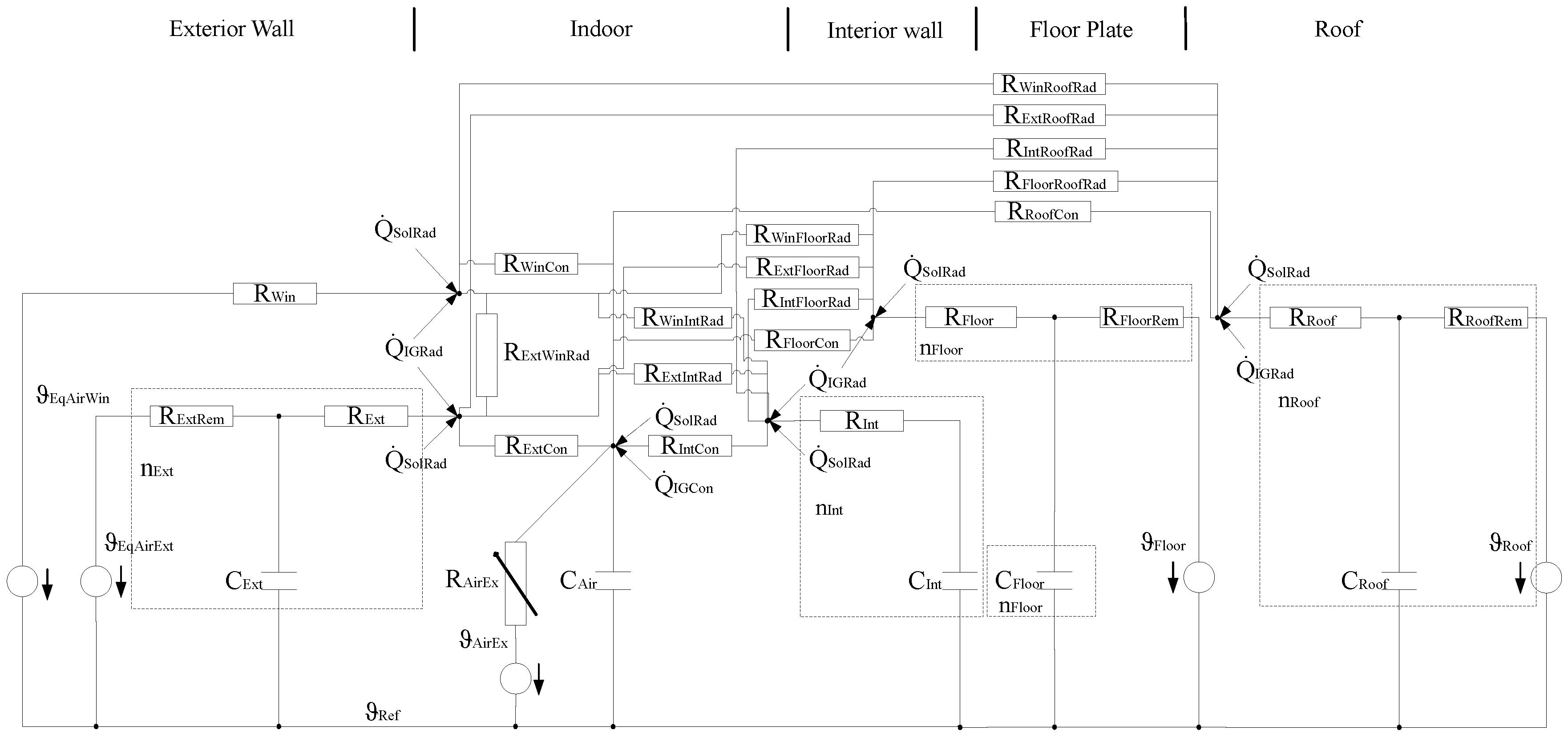
• Building thermal models simplification. Using low order RC models is a common approach.
• Definition of Archetypes/Prototypes models. Building types are categorized and a standard default model is defined for each category.
• Usage of BIM (Building Information Models) or dedicated city information models such as CityGML files.
• Individual parameters are often missing and then generated using statistical databases.

Among UBEM tools, TEASER is particularly adapted to the generation of low order models with few input data. This Python package developed at the University of Aachen can generate a simple “archetype” model of a building with a minimum of five parameters and can involve statistical databases for data enrichment. The generated models are Python objects translated in Modelica using IBPSA annex 60 or Aixlib libraries [40].

We build here “four walls elements (i.e., interior walls, exterior walls, floor plate, and roof) SingleFamilyDwelling” archetypes models using TEASER according to the IWU (Institut Wohnen und Umwelt—Institute for Housing and Environment) topology issued from the EPISCOPE project [36]. “SingleFamilyDwelling” corresponds to the archetype’s data enrichment method. At the moment, TEASER mostly supports archetypes issued from studies of the German stock. This is not an issue here since we only test our methodology, but the implementation of French archetypes should be necessary for more accurate results. The resulting model is a RC reduced-order thermal model corresponding to the “AixLib.ThermalZones.ReducedOrder.RC.FourElements” component of the AixLib Modelica Library [43], as depicted in Figure 4. The corresponding Modelica simulation is further used as a reference for the virtual district.

A second model is required to perform optimizations. Thus, we developed a simpler linear building model in OMEGAlpes. Furthermore, too many model parameters can be counterproductive for an early-stage study. Therefore, we implemented a simplified RC-model of the Swiss SIA2044 norm in OMEGAlpes meeting our main needs: it can be easily built with few data, all the equations are linear (described Figure 5), and the Swiss building structure is very similar to the French one.

This RC-model is composed of a thermal capacity C_m and five thermal resistances:

• H_EA: Heat transfer coefficient between the air node (a) and outdoor (e)
• H_EC: Heat transfer coefficient between the central node (c) and outdoor (e)
• H_EM: Heat transfer coefficient between the building mass node (m) and outdoor (e)
• H_AC: Heat transfer coefficient between the air node (a) and the central node (c)
• H_MC: Heat transfer coefficient between the building mass node (m) and the central node (c)

Parameters in TEASER models are translated to the OMEGAlpes model such that global thermal transfer coefficient (U) values and thermal capacitance are preserved.

2.3. Generation of the Building Stock Model from Existing Data

In our residential district study case, the following data are available:

• RSET files for eight buildings: These files stand for “Récapitulatif Standardisé d’Étude Thermique” (Standard Report of Thermal Study) and are mandatory in France for the construction of each new building since the application of the French thermal policy RT2012. Each of these files is an XML document containing relevant data such as U values, areas, structural information, HVAC devices description, and thermal performance coefficients.
• Grenoble city land registry: GeoJson file containing all building’s footprints. This file is issued from the Grenoble Open data portal [33].
• A spreadsheet issued from engineering studies gathering general information on district buildings (addresses, dates of construction, heights, and number of floors).
• A meteorological file of one year of data.
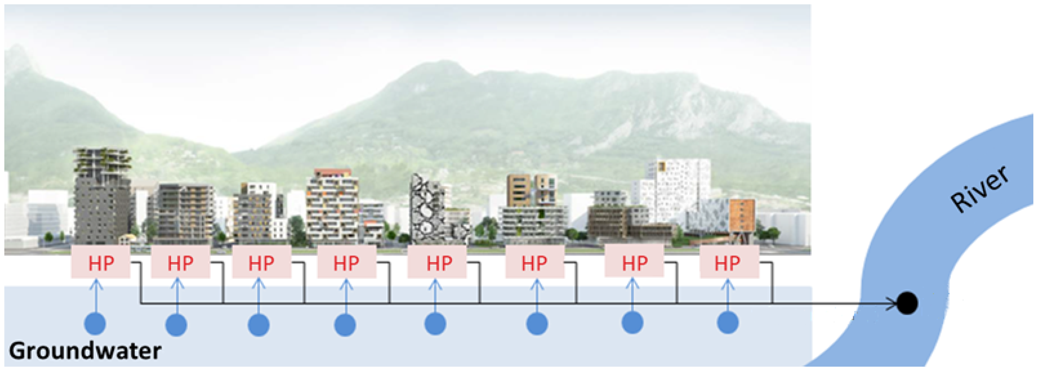
• Various documentation issued from engineering offices involved in the district construction (electrical network map, heat pumps datasheets, etc.)

For OMEGAlpes building models, we need the following data:

• U values and areas of ground floors, roofs, walls and windows
• Absorbtivity and emissivity of walls, roofs, and windows
• Transmittance of windows
• Surfaces areas
• Net leased area
• Number of floors
• Building height
• Building type (small, medium or heavy)

All the data required for OMEGAlpes building models can be deduced from generated TEASER models. Then, the UBEM generation is processed according with the workflow summarized in Figure 6.

In this workflow, one parses all the data files first. For buildings with RSET files, all the required parameters to build TEASER and OMEGAlpes models, except for emissivity, absorbtivity, and transmittance, are present. For other buildings, there are only enough data to generate TEASER archetypes. For some of them, the floor area is not directly available and one has to find corresponding polygons in the land registry file to estimate them. To complete missing data for OMEGAlpes models, one can extract parameters generated by TEASER in archetypes. For each parameter parsing, injection or extraction, one has to deal with different formulations and units. The generated dataset used to build all OMEGAlpes building models is summarized in Table 1.

To apply this workflow, we developed a specific Python package to ease file parsing, data manipulation (with an intermediate SQLite database) and district model generation, with modularity in mind (for further data integration). The architecture of this tool is summarized in Figure 7.

Such an approach is close to the ETL methodology. As ETL processes are well suitable for UML modeling [44], the choice of an Object-Oriented Programming language such as Python is appropriate. Besides, the support of Python by the scientific community eases the development of the “Transform” part.

3. Modeling of the Optimal Planning Problem

3.1. Optimal Planning of the District Heating Systems with OMEGAlpes

As already mentioned, two flexibility approaches to manage the district heating systems are addressed through the study case:

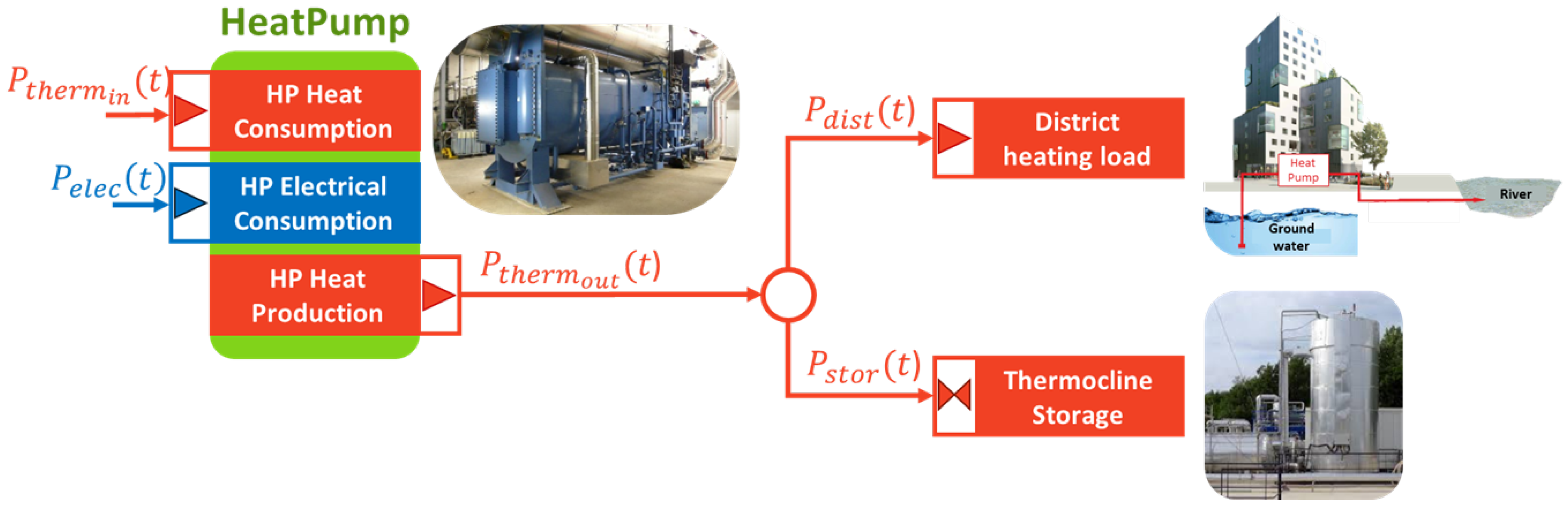
• The first one consists in designing an energy system composed of a heat pump and thermal energy storage to minimize the $C{O}_2$ emissions of a fixed district heating load.
• The second study case also aims to minimize the $C{O}_2$ emissions of the buildings’ heating load, but thanks to flexibility through building envelopes. In this case, specific building models dedicated to the optimization should be used to estimate how the load can be modulated.

In both studies, we aim to estimate the possibility to decrease the $C{O}_2$ emissions by designing and operating the system. The studies were conducted during two weeks in January, which usually represent the coldest period and are critical for the power system. Thus, the design of the system can be significant for the entire heating period. It is important to notice here that our goal is not to predict energy needs and $C{O}_2$ emissions for an entire year, but to be closer to the operation. Therefore, focusing on two weeks allows us to anticipate the possibility to pursue our work with a model predictive control approach thereafter.

To define the OMEGAlpes optimization models, a graphical formalism was defined to represent the energy units and power flows (see Figure 8).

Let us introduce Study Cases 1 and 2; the results are detailed in Section 4.

3.2. Study Case 1: Flexibility through Thermal Energy Storage (TES)

The first study case deals with energy flexibility provided by a Thermal Energy Storage (TES) to minimize the $C{O}_2$ emissions of the district heating load. The energy system studied is composed of the district heated by geothermal groundwater through a heat pump and thermal energy storage to provide demand-side management. The goal of this study case is to design the whole supplying system (heat pump and storage). To do so, we used three OMEGAlpes units to model the energy system: the district heating load, the heat pump, and the thermal energy storage, as shown in Figure 9.

3.2.1. Estimation of the District Heating Load

In this first study case, only the flexibility provided by the storage energy system is addressed so that the district heating load cannot be modulated and is thus an input of our optimization problem. To estimate the thermal needs of the district, we relied on results from a first optimization obtained with OMEGAlpes which can be considered as a temperature regulation simulation. All buildings were modeled as described in the previous section and set with standard occupancy schedules obtained by TEASER and a temperature set-point of 20 °C. The objective of the optimization is to minimize the sum of the over-heating and the result (see Figure 10) is taken as the dynamic thermal consumption of the district ${\mathrm{P}}_{dist}$(t). In this figure, we can notice that, during the days, the district heating load is very low. This could be explained by the high insulation of the buildings which require low consumption and thus can benefit from occupancy and solar gains to cover their needs.

3.2.2. Modeling of Heat Pump

Composed of new residential buildings, the district can be heated by low temperatures around 35 °C. With a groundwater temperature around 15 °C, this specificity allows the heat pump to reach a high Coefficient Of Performance (COP) of 5. Moreover, the temperature of the groundwater is assumed to be invariant so that we can consider the COP to be a constant equal to 5. Therefore, the heat pump is modeled by the relations between the thermal power provided by the groundwater $P_{{therm}_{in}}\left(t\right)$, the electrical power consumed by the heat pump $P_{elec}\left(t\right)$, the thermal power delivered $P_{{therm}_{out}}\left(t\right)$ and the COP, as described in Equation (1).

$$\left\{\begin{array}{cc}{P}_{{therm}_{in}}\left(t\right)+P_{elec}\left(t\right)=P_{{therm}_{out}}\left(t\right)\hfill & \\ P_{{therm}_{out}}\left(t\right)=COP\ast P_{elec}\left(t\right)\hfill & \mathrm{Where}:COP=5\hfill \end{array}\right.$$

(1)

In this study case, a trade-off was chosen between different levels of accuracy of the whole energy system modeling according to the uncertainties relating to the occupants’ behaviors. Indeed, as we aim to estimate orders of magnitude of the $C{O}_2$ emissions reduction obtained by heating flexibility, the modeling of the heating systems is very simplified. For further studies, a deeper level of modeling could be needed to provide a more accurate estimation.

3.2.3. Modeling of Thermal Energy Storage (TES)

Multiple types of thermal energy storage systems are used in the literature to smooth building thermal needs. However, the most widespread technology used remains water tanks for their simplicity and low costs.

The power stored to the TES $P_{stor}\left(t\right)$ is defined as the difference between the charging power $P_c\left(t\right)$ and the discharging power $P_d\left(t\right)$ as described by Equation (2).

$$\left\{\begin{array}{c}{P}_{stor}\left(t\right)=P_c\left(t\right)-P_d\left(t\right)\hfill \\ P_c\left(t\right)\ge 0\hfill \\ P_d\left(t\right)\ge 0\hfill \end{array}\right.$$

(2)

Moreover, the relation between the energy contained in the water tank $e\left(t\right)$ and the charging and discharging powers is defined by Equation (3). The storage capacity $C_{stor}$ is defined as the maximal value of $e\left(t\right)$.

$$\left\{\begin{array}{c}e(t+dt)=e\left(t\right)\ast (1-{\alpha }_{sd})+(P_c\ast {\eta }_c-\frac{P_d}{{\eta }_d})\ast dt\hfill \\ e\left(t_0\right)=e\left(t_f\right)\hfill \\ e\left(t\right)\le C_{stor}\hfill \end{array}\right.$$

(3)

where

• ${\alpha }_{sd}$ is the coefficient of self-discharge of the storage system (depending on the storage design). Here, the coefficient is a percentage per time step ($dt$ = 10 min).
• ${\eta }_c$/${\eta }_d$ is the charging/discharging efficiency (standard value of 95% corresponding to actual TES).
• $t_0$/$t_f$ is the starting/ending time step of the period.
• $dt$ is the time step (10 min).

In this study, a stratified storage system is considered called thermocline storage whose management is more complex than traditional storage (more details can be found in [45]). Indeed, in our case, we assumed that the storage has to be fully charged at least once per five days to optimally operate. The first step to model this constraint is to define a variable to indicate if the storage is fully charged. To do so, a binary variable was introduced: is_soc_max(t) which equals 0 when the state of charge is lower than 100% and 1 when the storage is fully charged. The definition of this indicator was realized thanks to Equation (4), where $C_{stor}$ is the storage capacity, $e_{stor}\left(t\right)$ is the energy contained in the storage at the time t and $ϵ$ is taken equal to 10⁻³.

$$\left\{\begin{array}{c}{C}_{stor}\ast (1+is\_soc\_max\left(t\right)-ϵ)\ge e_{stor}\left(t\right)\hfill \\ C_{stor}\ast is\_soc\_max\left(t\right)\le e_{stor}\left(t\right)\hfill \end{array}\right.$$

(4)

Then, our constraint can be expressed thanks to a sliding window including five days. Let $t_{cycl}$ be the time step corresponding to the end of the first five-day period; the constraint of at least one full charge during five days is defined by Equation (5).

$$\forall t\in [t_{cycl};t_f],\sum _{k=t-t_{cycl}}^{t}is\_soc\_max\left(k\right)\le 1$$

(5)

3.2.4. Modeling of $C{O}_2$ Emissions of the District Heating Load

In this study case, the $C{O}_2$ emissions of the district heating load ($E{m}_{C{O}_2}$) come from the electrical consumption of the heat pump. Fed by the French power system, the heat pump emissions vary dynamically according to the French grid $C{O}_2$ emissions rate ($e{m}_{C{O}_2,rate}\left(t\right)$, see Figure 11).

Thus, the $C{O}_2$ emissions of the district heating load can be calculated by Equation (6), so that changing the heat pump operation could lead to $C{O}_2$ reduction, which we tried to achieve thanks to thermal energy storage in this study case.

$$E{m}_{C{O}_2}=\sum _{t=t_0}^{t=t_f}{P}_{elec}\left(t\right)\ast e{m}_{C{O}_2,rate}\left(t\right)$$

(6)

3.2.5. Energy System Design Parameters

As explained above, the objective is to minimize the $C{O}_2$ emissions of the district heating load. To do so, we considered a groundwater source heat pump coupled with the thermal energy storage that we aim to design. Three parameters are optimized:

• The storage capacity ($C_{stor}$): Increasing the storage capacity allows more energy to be stored and thus the possibility to provide the thermal needs with the TES during high-$C{O}_2$ periods. However, big storage capacities induce higher costs and volume. In this study, we considered TES with capacity from 100 kWh to 48 MWh.
• The storage insulation, defined by the self-discharge coefficient (${\alpha }_{sd}$): An important factor in the storage design is the possibility to shift the energy in the medium term (several hours to days). This essentially depends on the self-discharge coefficient. If it is too high, too many losses will appear and it would be less efficient to shift the energy in the medium-term. In this study, we compared the influence of three values of ${\alpha }_{sd}$: 0.125%, 0.25% and 0.5%, each ten minutes.
• The maximal electrical power consumed by the heat pump ($P_{elec}^{max}$): Increasing the power that can be consumed by the heat pump leads to higher thermal power delivered at a low-$C{O}_2$ period. Nevertheless, it induces high consumption peaks that are usually harmful to the power grid. In this study, we went from no over-sizing of the heat pump (300 kW) to 2500 kW.

3.3. Study Case 2: Flexibility through Heating Loads Modulation (BaB)

In this second study case, thermal flexibility is provided by the building envelopes. Each building is modeled individually so that the district load can be deduced by the addition of each building heating load. Thus, the thermal load of the district can be directly modulated without any external thermal energy storage (see Figure 12).

3.3.1. Estimation of the District Heating Load

To guarantee the occupants’ thermal comfort, the operative temperature is constrained to be higher or equal to 20 °C. Thus, the building can be over-heated by moments to store heat into the buildings while keeping thermal comfort.

The heating load can be calculated for each time step according to the thermal RC model available in OMEGAlpes and presented in the previous section. Besides constraining the operative temperature, the boundaries conditions are the same as before. These internal gains (from occupancy and weather) are applied to the nodes a, c and m (see Figure 5). More details about the model can be found in [46].

3.3.2. Modeling of Heat Pumps and $C{O}_2$ Emissions of the District Heating Load

The configuration of the district is slightly changed since each building is fed by its heat pump. Each heat pump is designed with an over-sizing (around +66%) according to the reference heating need of being able to use flexibility. The total maximal electrical consumption allowed to feed all the heat pumps was set to 500 kW.

The modeling of the $C{O}_2$ emissions is similar to the previous study so that each heat pump emits according to its electrical consumption. However, the objective to minimize the $C{O}_2$ emissions is global.

In this study case, the energy system is designed before running the optimization. Therefore, the minimization of the $C{O}_2$ emissions is based on finding an optimal operation of all the heat pumps of the districts.

4. Results

This section is divided into two main subsections:

• Optimization: Presentation of the optimization results for the two study cases aiming to reduce the $C{O}_2$ emissions of the district heating load. Here, reduced building models are used to predict heating thermal needs.
• Simulation: A reference scenario is compared to the simulation results obtained by setting the temperature profile according to optimization results with flexibility.

4.1. Optimization

The study cases presented in this paper are realized for a time step of 10 min for two weeks in January. For the first one, each optimization problem generated is composed of 38k variables (28k continuous and 10k binaries) for 61k constraints. The resolution was launched on an Intel bicore i5 2.4 GHz CPU with the Gurobi solver so that the optimization problem was solved within less than 10 s on average for 192 optimizations. The corresponding results are detailed Section 4.1.2.

The second study case consists of a single resolution since only one configuration is studied. The associated optimization problem is composed of 1211k variables (1100k continuous and 111k binaries) for 1263k constraints. The resolution was launched on the same Intel bicore i5 2.4 GHz CPU with the Gurobi solver and the optimization problem was solved within 23 min. The dynamic results are detailed Section 4.1.3.

4.1.1. Flexibility Potential

To evaluate the gains obtained by optimization, the first step is to estimate the maximal reduction in $C{O}_2$ emissions that can be achieved. A simple way to evaluate this maximum is to allow shifting each 10-min power slot of the load curve to minimize the $C{O}_2$ while consuming the same energy during the two weeks. In this case, the $C{O}_2$ emissions can be reduced to a maximum of 22% keeping the current heat pump maximal power consumption (300 kW). Of course, in this case, the building comfort (internal temperature) is not guaranteed. This potential of 22% $C{O}_2$ savings is used to compare the next results.

The dynamic result of this naive estimation is shown Figure 13. We can notice that some $C{O}_2$ emissions reduction can be obtained by anticipating or removing the consumption for a few hours (short-term flexibility), but the longer-term variation of the $C{O}_2$ levels lead to a need for longer-term flexibility.

4.1.2. Study Case 1: Flexibility through Thermal Energy Storage (TES)

In this study case, three elements were designed: the storage capacity ($C_{stor}$), the storage self-discharge coefficient (${\alpha }_{sd}$) and the maximal electrical power consumed by the heat pump ($P_{elec}^{max}$). Results are shown in Figure 14 for the three self-discharge coefficients studied (0.125%, 0.25% and 0.5%). The $C{O}_2$ emissions reduction obtained in each configuration is drawn according to the storage capacity and the maximal electrical power consumed by the heat pump.

Regarding the storage capacity, we can notice that 100 kWh is too small to reduce the $C{O}_2$ emissions regardless of the two other parameters. For larger capacities (≥1 MWh), the impact on the $C{O}_2$ emissions reduction begins to be noticeable and is strongly correlated with the self-discharge coefficient and the maximal power consumed by the heat pump.

For a storage capacity under 2 MWh, we can notice that the reduction in $C{O}_2$ emissions are lower than 3.5% for all designs. However, in the case of a TES of 48 MWh with 0.125% of self-discharge and a maximal electrical power of the heat pump of 2500 MW, we manage to reach 20% reduction in $C{O}_2$ emissions of the district heating load. Knowing that the average daily heating consumption of the district during the period is 8 MWh, a 4 MWh storage corresponds to 12 h of consumption while a capacity of 48 MWh corresponds to six days.

Two phenomena happen when designing the energy system to use flexibility to reduce $C{O}_2$ emissions:

• The ability to store in the long-run: defined by the storage capacity and by the self-discharge coefficient. Indeed, with relatively poor insulation (${\alpha }_{sd}$ = 0.5%), increasing the storage capacity beyond 8 MWh has no significant effect because of the importance of losses for long-term storage. However for a higher quality of insulation (${\alpha }_{sd}$ = 0.125%), increasing the capacity until 48 MWh is always beneficial from an environmental point of view.
• The possibility to store a lot of energy during low-$C{O}_2$ periods: defined by the charging power of the storage and by the maximal power that can be consumed by the heat pump. In the case of a TES with a 48 MWh capacity and a 0.5% self-discharge coefficient, increasing the maximal power consumed by the heat pump from 300 kW to 2500 kW saves from 3.9% to 6.2%. Indeed, with higher electrical consumption, the heat pump can provide more low-$C{O}_2$ thermal power to the storage.

Although it seems reachable to have a strong impact on the $C{O}_2$ emissions of the district heating load with a big TES and a heat pump with high electrical power needs, this design choice leads to other problems. Indeed, choosing the kind of heat pumps means to increase the electrical power peaks and could report $C{O}_2$ emissions decreases from the heating side to increases at the electrical one. Over-sizing the heat pump should thus be carefully considered taking this effect in mind. Moreover, a 48 MWh water tank is expensive and takes a lot of space so that it is not an ideal solution. Nevertheless, it could be very interesting to deeply consider the level of insulation that can have an important impact.

Finally, using a building’s envelope as storage should be investigated.

4.1.3. Study Case 2: Flexibility through Heating Loads Modulation

In this case, the $C{O}_2$ reduction is low (0.5%). Although the flexibility potential was previously estimated to 22%, it mainly relies on medium- and long-term flexibility. However, with the Building as Battery (BaB) concept, the flexibility addressed in our case can be defined as short term. Indeed, we can notice on the optimization results (Figure 15) that no energy is shifted for more than one day. High consumption peaks allow profiting from low-$C{O}_2$ rate periods but the energy cannot be stored in the long run. Indeed, with external wall insulation systems (EWIS), buildings envelopes form a relatively small storage capacity, while the $C{O}_2$ variability is more long-term in this case.

Moreover, over-heating the buildings leads to an increase in district energy consumption (0.9%), so that the environmental gain due to shifting the heating load is reduced. However, the mean operative temperature goes from 20.3 °C to 20.4 °C, i.e., an increase of 0.1 °C (0.4%). Therefore, the increase of the consumption induces a better thermal comfort while reducing $C{O}_2$ emissions. Many studies achieve a greater reduction by allowing over- and under-heating [47], i.e., by using both energy flexibility and sobriety, while we choose to focus on the impact of flexibility only.

With a maximal electrical consumption of heat pumps of 500 kW, this scenario can be compared to those with a single 500 kW heat pump. The reduction of $C{O}_2$ emissions obtained by buildings as storage is similar to results with a TES with a capacity between 100 kWh and 1 MWh, whatever the self-discharge coefficient.

Finally, the reference scenario is the result of an optimization problem by providing minimal energy to maintain thermal comfort. Thus, when over-heating is not compensated by the $C{O}_2$ diminution, the $C{O}_2$ emissions minimization corresponds to the energy minimization.

For this reason, we need to compare a simulation reference profile to the flexible scenario to see if the improvement is preserved with a standard controller. Besides, comparing OMEGAlpes results with simulation can lead to investigating optimal control robustness during application.

4.2. Simulation

Experimenting flexibility scenarios computed by OMEGAlpes directly on the real district is a complex task. Before performing these tests, we started simulation studies to validate our approach and/or identify the main issues towards implementation. Since we used TEASER as an intermediate for building OMEGAlpes models, Modelica models are also ready to simulate for each building. First, we can compare heating needs and operative temperature profiles (defined as a mean between air and radiant temperatures) for both modeling approaches. To do so, we used two specific control scenarios:

• Constant temperature setp oint: In this case, we want to achieve a constant operative temperature of 20 °C inside each building. With Modelica models, it consists in inserting an operative temperature sensor and regulating the injected heat power with a PI controller. In the case of OMEGAlpes models, the heat demand is computed to minimize the discrepancy between buildings operative temperatures and the 20 °C set point.
• Flexibility scenario: In the optimization case presented above, OMEGAlpes has reduced energy consumption and $C{O}_2$ emissions while preserving thermal comfort constraints. To reproduce computed power shifts on Modelica models, we applied the operative temperatures computed for the flexibility scenario as a new setp oint profile.

In the first case of constant temperature set point, we obtained the results presented in Figure 16 (buildings mean operative temperatures and the sum of all buildings consumption).

The first obvious difference stands in energy needs. Modelica models generated by TEASER have a more important consumption for the same comfort criteria and are therefore probably less insulated. Besides, temperature peaks are shifted between models. These shifts can be due to the differences in control strategies, and/or in computed internal gains despite using the same scenarios and weather files. Consequently, even with the same data sources, it appears hard to obtain identical dynamic behaviors between different modelers. Further effort must be invested to preserve global building characteristics during model translating (in our case, model simplification). Besides, this also suggests the use of a model calibration phase before implementing any model-based control strategy.

If we consider the application of the flexibility scenario in Figure 17, the consumption differences between both models are visually less important, except for higher spikes for Modelica models, but dynamics of operative temperature are sill very present (more inertia to go down for Modelica models).

We also compared performance results between constant temperature set point and computed flexibility temperatures on Modelica models only, to see if it also leads to improvement despite model discrepancies (see Figure 18).

Here, the dynamics induced by the flexibility scenario are very noticeable. As for OMEGAlpes results, we observe power shifts and spikes inducing heat storage in buildings envelopes. Unfortunately, performance is not preserved, since both energy consumption and $C{O}_2$ emissions are worsened (

Table 2. Performance indices with flexibility scenario to optimize $C{O}_2$ emissions against constant temperature setpoint.

	Energy Consumption	${\mathit{CO}}_2$ Emissions
Improvement with OMEGAlpes model	−0.78%	0.41%
Improvement with Modelica model	−2.28%	−0.63%

).

This implies that the flexibility command computed here is not robust to the model discrepancies we are facing. Therefore, the robustness of flexibility scenarios towards modeling uncertainties is certainly a key research topic before real-life integration if we do not want optimized scenarios to be counterproductive. This is also true during the early stage of design where low order models are used to investigate energy scenarios.

5. Conclusions

Based on an ETL (Extract–Transform–Load) method, we have initiated a tool based on the heterogeneous available data of buildings at the district scale, which can generate the necessary data for optimization and simulation models. In particular, we have applied this method to the case of data available on a new residential district composed of 16 residential buildings. This work makes it possible to identify the important parameters for different modeling tools at the neighborhood scale, to extract them from available data, or to estimate them when they are not available.

We then carried out two flexibility studies, based on the OMEGAlpes tool, which requires modeling in MILP formulation. The first study analyzed the design of a heat pump (nominal power) and storage (capacity and self-discharge factor) to desynchronize the production of heat and use to heat buildings. It appears that a large investment is necessary to try to reach the maximum potential (estimated at 22%), which relies in particular on long-term flexibility (more than a week). The second study relied on thermal storage via the building envelope. This zero investment solution is, therefore, a potential alternative to the previous case. However, the results obtained below 1% show that the low storage capacity of these residential buildings does not allow addressing flexibility considering a $C{O}_2$ variability during several days.

Finally, the tool we developed for data processing at the neighborhood scale allowed us to easily set up a validation process. Thus, we have transmitted the flexibility results in the simulation model using the Modelica AixLib library. The results show a predicted performance degradation compared with optimization results. On very small gains (<1%) obtained by the upward flexibility (temperature > 20 °C), it even presents negative performance in energy and $C{O}_2$. This lack of robustness to modeling assumptions reinforces the idea that a tool to generate different levels of modeling based on available data will be indispensable for future studies related to robustness in optimization.

References

1. Climate Action Tracker—EU. Available online:. Available online: https://climateactiontracker.org/countries/eu/ (accessed on 30 July 2019).
2. International Energy Agency. Buildings. Available online: https://www.iea.org/topics/energyefficiency/buildings/ (accessed on 30 July 2019).
3. Kammen, D.M.; Sunter, D.A. City-integrated renewable energy for urban sustainability. Science 2016, 352, 922–928. [Google Scholar] [CrossRef] [PubMed] [Green Version]
4. Henning, D. MODEST—An energy-system optimisation model applicable to local utilities and countries. Energy 1997, 22, 1135–1150. [Google Scholar] [CrossRef]
5. Howells, M.; Rogner, H.; Strachan, N.; Heaps, C.; Huntington, H.; Kypreos, S.; Hughes, A.; Silveira, S.; DeCarolis, J.; Bazillian, M.; et al. OSeMOSYS: The Open Source Energy Modeling System: An introduction to its ethos, structure and development. Energy Policy 2011, 39, 5850–5870. [Google Scholar] [CrossRef]
6. Gardumi, F.; Shivakumar, A.; Morrison, R.; Taliotis, C.; Broad, O.; Beltramo, A.; Sridharan, V.; Howells, M.; Hörsch, J.; Niet, T.; et al. From the development of an open-source energy modelling tool to its application and the creation of communities of practice: The example of OSeMOSYS. Energy Strategy Rev. 2018, 20, 209–228. [Google Scholar] [CrossRef]
7. Messner, S.; Schrattenholzer, L. MESSAGE–MACRO: Linking an energy supply model with a macroeconomic module and solving it iteratively. Energy 2000, 25, 267–282. [Google Scholar] [CrossRef]
8. Loulou, R.; Labriet, M. ETSAP-TIAM: The TIMES integrated assessment model Part I: Model structure. Comput. Manag. Sci. 2008, 5, 7–40. [Google Scholar] [CrossRef]
9. Loulou, R. ETSAP-TIAM: The TIMES integrated assessment model. Part II: Mathematical formulation. Comput. Manag. Sci. 2008, 5, 41–66. [Google Scholar] [CrossRef]
10. Prospective Outlook on Long-Term Energy Systems. Available online: https://ec.europa.eu/jrc/en/poles (accessed on 30 July 2019).
11. Criqui, P.; Mima, S.; Viguier, L. Marginal abatement costs of CO2 emission reductions, geographical flexibility and concrete ceilings: An assessment using the POLES model. Energy Policy 1999, 27, 585–601. [Google Scholar] [CrossRef]
12. Cochran, J.; Bird, L.; Heeter, J.; Arent, D. Integrating Variable Renewable Energy in Electric Power Markets: Best Practices from International Experience; (No. NREL/TP-6A20-53732); National Renewable Energy Lab. (NREL): Golden, CO, USA, 2012.
13. Taibi, E.; Nikolakakis, T.; Gutierrez, L.; Fernandez, C.; Kiviluoma, J.; Rissanen, S.; Lindroos, T.J. Power System Flexibility for the Energy Transition: Part 1, Overview for Policy Makers; International Renewable Energy Agency IRENA: Abu Dhabi, UAE, 2018. [Google Scholar]
14. Lund, P.D.; Lindgren, J.; Mikkola, J.; Salpakari, J. Review of energy system flexibility measures to enable high levels of variable renewable electricity. Renew. Sustain. Energy Rev. 2015, 45, 785–807. [Google Scholar] [CrossRef] [Green Version]
15. Mendes, G.; Loakimidis, C.; Ferrão, P. On the planning and analysis of Integrated Community Energy Systems: A review and survey of available tools. Renew. Sustain. Energy Rev. 2011, 15, 4836–4854. [Google Scholar] [CrossRef]
16. Keirstead, J.; Jennings, M.; Sivakumar, A. A review of urban energy system models: Approaches, challenges and opportunities. Renew. Sustain. Energy Rev. 2012, 16, 3847–3866. [Google Scholar] [CrossRef] [Green Version]
17. Allegrini, J.; Orehounig, K.; Mavromatidis, G.; Ruesch, F.; Dorer, V.; Evins, R. A review of modelling approaches and tools for the simulation of district-scale energy systems. Renew. Sustain. Energy Rev. 2015, 52, 1391–1404. [Google Scholar] [CrossRef]
18. HOMER—Hybrid Renewable and Distributed Generation System Design Software. Available online: https://www.homerenergy.com/ (accessed on 30 July 2019).
19. Simpkins, T.; Cutler, D.; Anderson, K.; Olis, D.; Elgqvist, E.; Callahan, M.; Walker, A. REopt: A platform for energy system integration and optimization. In Proceedings of the ASME 2014 8th International Conference on Energy Sustainability Collocated with the ASME 2014 12th International Conference on Fuel Cell Science, Engineering and Technology, Boston, MA, USA, 30 June–2 July 2014; pp. ES2014-6570, V002T03A006. [Google Scholar]
20. Artelys | Optimization Solutions—Artelys Crystal City. Available online: https://www.artelys.com/fr/crystal/city/ (accessed on 30 July 2019).
21. Bollinger, L.A.; Dorer, V. The Ehub Modeling Tool: A flexible software package for district energy system optimization. Energy Procedia 2017, 122, 541–546. [Google Scholar] [CrossRef]
22. Distributed Energy Resources—Customer Adoption Model (DER-CAM) | Building Microgrid. Available online: https://building-microgrid.lbl.gov/projects/der-cam (accessed on 30 July 2019).
23. Hilpert, S.; Kaldemeyer, C.; Krien, U.; Günther, S.; Wingenbach, C.; Plessmann, G. The Open Energy Modelling Framework (oemof)—A new approach to facilitate open science in energy system modelling. Energy Strategy Rev. 2018, 22, 16–25. [Google Scholar] [CrossRef]
24. Atabay, D. An open-source model for optimal design and operation of industrial energy systems. Energy 2017, 121, 803–821. [Google Scholar] [CrossRef]
25. Ringkjøb, H.K.; Haugan, P.M.; Solbrekke, I.M. A review of modelling tools for energy and electricity systems with large shares of variable renewables. Renew. Sustain. Energy Rev. 2018, 96, 440–459. [Google Scholar] [CrossRef]
26. Pipattanasomporn, M.; Kuzlu, M.; Rahman, S.; Teklu, Y. Load Profiles of Selected Major Household Appliances and Their Demand Response Opportunities. IEEE Trans. Smart Grid 2013, 5, 742–750. [Google Scholar] [CrossRef]
27. Laicane, I.; Blumberga, D.; Blumberga, A.; Rosa, M. Reducing Household Electricity Consumption through Demand Side Management: The Role of Home Appliance Scheduling and Peak Load Reduction. Energy Procedia 2015, 72, 222–229. [Google Scholar] [CrossRef] [Green Version]
28. Reynders, G.; Nuytten, T.; Saelens, D. Potential of structural thermal mass for demand-side management in dwellings. Build. Environ. 2013, 64, 187–199. [Google Scholar] [CrossRef]
29. Oliveira Panão, M.J.N.; Mateus, N.M.; Carrilho da Graça, G. Measured and modeled performance of internal mass as a thermal energy battery for energy flexible residential buildings. Appl. Energy 2019, 239, 252–267. [Google Scholar] [CrossRef]
30. Arteconi, A.; Polonara, F.; Arteconi, A.; Polonara, F. Assessing the Demand Side Management Potential and the Energy Flexibility of Heat Pumps in Buildings. Energies 2018, 11, 1846. [Google Scholar] [CrossRef]
31. Le Dréau, J.; Heiselberg, P. Energy flexibility of residential buildings using short term heat storage in the thermal mass. Energy 2016, 111, 991–1002. [Google Scholar] [CrossRef]
32. Pajot, C.; Morriet, L.; Hodencq, S.; Reinbold, V.; Delinchant, B.; Wurtz, F.; Maréchal, Y. Omegalpes: An Optimization Modeler as an Efficient Tool for Design and Operation for City Energy Stakeholders and Decision Makers. In Proceedings of the 2019 IBPSA Building Simulation International Conference, Rome, Italy, 2–4 September 2019. [Google Scholar]
33. Data MetropoleGrenoble—Saisissez vous des Données. Available online: http://data.metropolegrenoble.fr/ (accessed on 30 July 2019).
34. EU Buildings Database. Available online: https://ec.europa.eu/energy/en/eu-buildings-database (accessed on 30 July 2019).
35. PSS—ARCHI, EU. Available online:. Available online: http://www.pss-archi.eu/ (accessed on 30 July 2019).
36. Joint Website of the TABULA and EPISCOPE Projects. Available online: http://episcope.eu/welcome/ (accessed on 30 July 2019).
37. Kimball, R.; Caserta, J. The Data Warehouse ETL Toolkit: Practical Techniques for Extracting, Cleaning, Conforming, and Delivering Data; John Wiley & Sons, Wiley Publishing Inc.: Indianapolis, IN, USA, 2011. [Google Scholar]
38. Walter, E.; Kämpf, J.H. A verification of CitySim results using the BESTEST and monitored consumption values. In Proceedings of the 2nd Building Simulation Applications Conference, Bolzano, Italy, 4–6 February 2015; pp. 215–222. [Google Scholar]
39. Fonseca, J.A.; Nguyen, T.A.; Schlueter, A.; Marechal, F. City Energy Analyst (CEA): Integrated framework for analysis and optimization of building energy systems in neighborhoods and city districts. Energy Build. 2016, 113, 202–226. [Google Scholar] [CrossRef]
40. Remmen, P.; Lauster, M.; Mans, M.; Fuchs, M.; Osterhage, T.; Müller, D. TEASER: An open tool for urban energy modelling of building stocks. J. Build. Perform. Simul. 2018, 11, 84–98. [Google Scholar] [CrossRef]
41. Chen, Y.; Hong, T.; Piette, M. Automatic Generation and Simulation of Urban Building Energy Models Based on City Datasets for City-Scale Building Retrofit Analysis. Appl. Energy 2017, 205. [Google Scholar] [CrossRef]
42. Sola, A.; Corchero, C.; Salom, J.; Sanmarti, M. Simulation tools to build urban-scale energy models: A review. Energies 2018, 11, 3269. [Google Scholar] [CrossRef]
43. Lauster, M. AixLib.ThermalZones.ReducedOrder.RC.FourElements. Available online: https://build.openmodelica.org/Documentation/AixLib.ThermalZones.ReducedOrder.RC.FourElements.html (accessed on 30 July 2019).
44. Trujillo, J.; Luján-Mora, S. A UML Based Approach for Modeling ETL Processes in Data Warehouses. In Proceedings of the International Conference on Conceptual Modeling, Chicago, IL, USA, 13–16 October 2003. [Google Scholar]
45. Raccanello, J.; Rech, S.; Lazzaretto, A. Simplified dynamic modeling of single-tank thermal energy storage systems. Energy 2019, 182, 1154–1172. [Google Scholar] [CrossRef]
46. Pajot, C.; Delinchant, B.; Maréchal, Y.; Artiges, N. Building Reduced Model for MILP Optimization: Application to Demand Response of Residential Buildings. In Proceedings of the 2019 IBPSA Building Simulation international conference, Rome, Italy, 2–4 September 2019. [Google Scholar]
47. Kampelis, N.; Sifakis, N.; Kolokotsa, D.; Gobakis, K.; Kalaitzakis, K.; Isidori, D.; Cristalli, C. HVAC Optimization Genetic Algorithm for Industrial Near-Zero-Energy Building Demand Response. Energies 2019, 12, 2177. [Google Scholar] [CrossRef]
Figure 1. Illustration of the district thermal fed by a groundwater source.
Energies 12 03632 g001
Figure 2. Grenoble “Cambridge Eco-district” overview.
Energies 12 03632 g002
Figure 3. Data heterogeneity in districts.
Energies 12 03632 g003
Figure 4. Four elements building model generated by TEASER [43].
Energies 12 03632 g004
Figure 5. RC model according to SIA 2044.
Energies 12 03632 g005
Figure 6. Workflow for district model generation.
Energies 12 03632 g006
Figure 7. Python software architecture for data handling and model generation.
Energies 12 03632 g007
Figure 8. OMEGAlpes formalism for energy system modeling.
Energies 12 03632 g008
Figure 9. Modeling of the energy system of the first study case (heat pump, district heating load and thermal energy storage) according to OMEGAlpes formalism.
Energies 12 03632 g009
Figure 10. District heating load during a two-week period in January obtained by optimization.
Energies 12 03632 g010
Figure 11. C O 2 emissions rate of the French power system during a two-week period in January 2018.
Energies 12 03632 g011
Figure 12. Modeling of the energy system of the second study case (16 buildings and 16 heat pumps) according to OMEGAlpes formalism.
Energies 12 03632 g012
Figure 13. Theoretical maximal flexibility to minimize C O 2 emissions by shifting 10-min values from the reference profile.
Energies 12 03632 g013
Figure 14. C O 2 emissions reduction according to the design of the heat pump and energy storage system.
Energies 12 03632 g014
Figure 15. Optimal flexibility to minimize C O 2 emissions by allowing over-heating.
Energies 12 03632 g015
Figure 16. Comparison between Modelica and OMEGAlpes—Constant temperature set point scenario.
Energies 12 03632 g016
Figure 17. Comparison between Modelica and OMEGAlpes—flexibility scenario.
Energies 12 03632 g017
Figure 18. Modelica simulations—comparison between control scenarios.
Energies 12 03632 g018